Entropy-Randomized Forecasting of Stochastic Dynamic Regression Models

Abstract

We propose a new forecasting procedure that includes randomized hierarchical dynamic regression models with random parameters, measurement noises and random input. We developed the technology of entropy-randomized machine learning, which includes the estimation of characteristics of a dynamic regression model and its testing by generating ensembles of predicted trajectories through the sampling of the entropy-optimal probability density functions of the model parameters and measurement noises. The density functions are determined at the learning stage by solving the constrained maximization problem of an information entropy functional subject to the empirical balances with real data. The proposed procedure is applied to the randomized forecasting of the daily electrical load in a regional power system. We construct a two-layer dynamic model of the daily electrical load. One of the layers describes the dependence of electrical load on ambient temperature while the other simulates the stochastic quasi-fluctuating temperature dynamics.

1. Introduction

Due to the gradually increasing resources and computational power of computers, huge amounts of data can be accumulated and stored, both in natural and digitized formats. Then, the following question arises immediately: what should be done with these data, except for storage? Extracting new knowledge from data seems to be a very interesting idea. The concepts of Data Mining (DM) [1,2], Big Data (BD) [3] and Data Science (DS) [4] were formulated and further developed by researchers accordingly.

A very tempting goal—extracting new knowledge from data—inevitably leads to the verbal or formal (mathematical) modeling of the “expected” knowledge. Therefore, any model has some predictive properties, which can be implemented only under known values of its quantitative characteristics (parameters). Data are a fundamental component of the three concepts above: data are adopted for estimating the characteristics of a model using machine learning (ML) procedures, which allows extracting new knowledge.

Unlike DM, BD, and DS, the concept of ML has a rich history of over 70 years as well as vast experience in solving numerous problems. The first publication in this field of research dates back to 1957; see [5]. The notion of empirical risk, a key element of ML procedures, was introduced in 1970 in the monograph [6]. The method of potential functions for classification and recognition problems was also presented in 1970 in another monograph [7]. The modern concept of ML is based on the deterministic parametrization of models and estimates using data sets with postulated properties. The quality of estimation is characterized by empirical risk functions, and their minimization gives optimal estimates [8,9].

As a rule, real problems that are solved by ML procedures are immersed in some uncertain environment. If the matter concerns data, they are acquired with inevitable errors, omissions or low reliability. The design and parametrization of models is a non-formalizable and subjective process that depends on the individual knowledge of a researcher. Therefore, in the mass application of ML procedures, the level of uncertainty is quite high.

All these circumstances indicate that it is necessary to somehow compensate uncertainty. Here a general trend is the application of its stochastic description to parametrized models and data. This means that the model parameters are assumed to be random (appropriately randomized), and the data are assumed to have random errors. Machine learning procedures with these properties belong to the class of randomized machine learning (RML) procedures. Their difference from the conventional ML procedures is that optimal estimates are constructed not for the parameters but for the probability density functions (PDFs) of the random parameters and the PDFs of the worst-case random errors in the data. In the entropy-based RML procedures, the functional of generalized information entropy [10] is used as an optimality criterion for estimates.

The core of an RML procedure is a parametrized predictive model designed for simulating the temporal (or spatiotemporal) evolution of a process under study. Therefore, such a model belongs to the class of dynamic models. Parametric dynamic regression models (PDRMs) are most widespread representatives of this class, in which the current state of a model is determined by its past states on a certain time interval [11,12]. A formal image of PDRMs is difference equations, in the general case of the pth order [13]. Most applications are described by linear PDRMs. In particular, they naturally occur in many problems of macroeconomic modeling and forecasting, e.g., time series analysis of economic indices [14], adequacy analysis of PDRMs [15], and prediction of exchange rates [16]. Linear PDRMs are effective enough for short-term forecasting, yet causing significant errors on large forecasting horizons. Therefore, attempts to improve forecasts by introducing various nonlinearities into PDRMs are quite natural. The monograph [17] was dedicated to a general approach to the formation and use of nonlinear PDRMs. However, applications require a more “personalized” approach to choosing the most useful and effective nonlinearity. On this pathway, it seems fruitful, e.g., to forecast exchange rates using logistic and exponential nonlinearities [18], or to predict the daily electrical load of a power system using periodic autoregressive models [19] or multidimensional time series [20].

Since forecasting is performed under uncertainty, the resulting errors caused by some unaccounted factors are often compensated, if possible, by assigning some probabilities to forecasts [21,22]. The most common approach is the use of Bayes’ theorem on posterior probability. Let a parametrized conditional probability density function of data and an a priori probability density function of parameters be specified; then their normalized product will determine the posterior probability density function of the parameters under fixed data. Fundamental problems in this field of investigations are connected with the structural choice of the conditional and prior PDFs. Typically, Gaussian PDFs or their mixture are selected, and the mixture weights are estimated using retrospective data [23,24,25]. A similar approach was adopted in applications: population genetics [26], where the method of numerical approximation of posterior PDFs was developed; the interaction between the financial sector of the economy and the labor market [27], where the Metropolis–Hastings algorithm was used to estimate the parameters of the above PDFs; population dynamics [28], where a hierarchy of Bayesian models was designed to predict fertility, mortality and migration rates. Probabilistic forecasts are constructed by other methods, taking into account the specifics of applications. In meteorology, retrospective weather forecasts are accumulated for estimating the PDFs; subsequently, these PDFs are used for short-term forecasting [29,30,31,32]. A rather interesting procedure is to form a probabilistic forecast as a mixture of forecasts obtained by different methods [33].

In this paper, we propose a fundamentally different forecasting method—the so-called entropy-randomized forecasting (ERF). In accordance with this method, an ensemble of random forecasts is generated by a predictive dynamic regression model (PDRM) with random input and parameters. The corresponding probabilistic characteristics, namely the probability density functions, are determined using the entropy randomized machine learning procedure. The ensembles of forecasting trajectories are constructed by the sampling of the entropy-optimal PDFs.

The proposed method is adopted for randomized prediction of the daily electrical load of a regional power system. A hierarchical randomized dynamic regression model that describes the dependence of the load on the ambient temperature is constructed. The temporal evolution of the ambient temperature is represented by an oscillatory second-order dynamic regression model with a random parameter and a random input. The results of randomized learning of this model on the GEFCom2014 dataset [34] are given. A randomized forecasting technology is suggested and its adequacy is investigated depending on the length of forecasting horizon.

2. Procedure of Entropy-Randomized Forecasting

Randomization as a means of imparting artificial and rationally organized random properties to naturally nonrandom events, indicators, or methods is a fairly common technique that yields a positive effect. There exist many examples in various fields of science, management, economics: randomized numerical optimization methods [35,36]; the mixed (random) strategies of trading on a stock exchange [37]; the randomized forecasting of population dynamics [38]; vibration control of industrial processes [39]. As the result of randomization, nonrandom objects gain artificial stochastic properties with optimal probabilistic characteristics in a chosen sense. The question on appropriate quantitative characteristics of optimality has always been controversial and ambiguous. It requires arguments that would somehow reflect the important specifics of a randomized object. In particular, a fundamental feature of forecasting procedures is uncertainty in the data, predictive models, methods for generating forecasts, etc.

In what follows, information entropy [40] will be used as a characteristic of uncertainty. In the works [41,42,43], using the first law of thermodynamics it was demonstrated that entropy is a natural functional describing the processes of universal evolution. Moreover, in accordance with the second law of thermodynamics, entropy maximization determines the best state of an evolutionary process under the worst-case external disturbance (maximum uncertainty). Also, note another quality of information entropy associated with measurement errors and other types of errors, which are important attributes of data: with the factor of such errors being considered in terms of informational entropy, the probabilistic characteristics of noises exerting the worst-case impact on forecasting procedures can be estimated in explicit form.

The technology of entropy-randomized forecasting consists of the following stages. At the beginning (the first stage), a predictive randomized model (PRM) of a studied object is formed and its parameters are designed. A PRM transforms real data into a model output. In the general case, these transformations are assumed to be dynamic, i.e., the model output observed at a time instant n depends on the states observed on some past interval. The PRM parameters are assumed to be of the interval type and random, and their probabilistic properties are characterized by the corresponding PDFs.

The second stage of the technology under consideration—randomized machine learning (more specifically, its entropy version)—is intended to estimate the PDFs. At this stage, the estimates of the PDFs are calculated using learning data sets and also a learning algorithm in the form of a functional entropy-linear programming problem.

At the third stage, the optimized PRM (with the entropy-optimal PDFs) is tested using a test data set and accepted quantitative characteristics of the quality of learning. The optimized PRM actually generates an ensemble of random trajectories, vectors, or events with the entropy-optimal values of their parameters.

The learned and tested PRMs serve for forecasting. In this case, the ensembles of random forecasted trajectories generated by the entropy-optimal PRMs are used to calculate their numerical characteristics such as mean trajectories, variance curves, median trajectories, the PDF evolution of forecasted trajectories, etc.

3. Randomized Dynamic Regression Models with Random Input and Parameters

Randomized dynamic regression models (RDRMs) form a class of dynamic models with random parameters that describe a parametrized dependence of the object’s state at a given time instant on external factors and its states at some past time instants.

The structures of models are designed on the basis of existing knowledge and hypotheses about the properties of an object, which often turn out to be very inaccurate. Moreover, the external factors themselves can change over time and therefore should be predicted to model the object’s dynamics. Reliable information on realistically measured impacts leading to the temporal evolution of external factors is often unavailable. The aforementioned indicates the presence of uncertainty, both in the development and further use of models. In [10], a method for reducing the influence of uncertainty based on the randomization of models (including the class of RDRMs) was proposed. In the latter case, this method extends the idea of randomization to the modeling of external factors and their evolution.

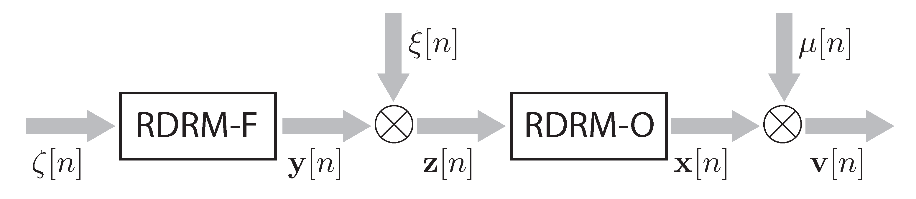
The structure of the RDRM is shown in Figure 1. It consists of a model of the main object (RDRM-O) with random parameters $\mathbf{a}\in R^p$ and a model of external factors (RDRM-F) with random parameters $\mathbf{b}\in R^s$ and a random input $\zeta \in R^q.$ The states of the object and its model belong to the vector space $R^m$, in which $\widehat{\mathbf{x}}\left[n\right]$ are the state vectors of the object and $\mathbf{x}\left[n\right]\in R^m$ are the state vectors of RDRM-O. The external factors are characterized by the vector $\widehat{\mathbf{y}}\left[n\right]\in R^q$ while the changes in the state of RDRM-F over time by the vector $\mathbf{y}\left[n\right]\in R^q.$ The variable n denotes discrete time taking integer values on the interval $\mathcal{L}=[n^{-},n^{+}].$

Consider the linear version of RDRM-O. Its state $\mathbf{x}\left[n\right]$ at a time instant n is changing under the influence of p retrospective states $\mathbf{x}[n-1],\cdots ,\mathbf{x}[n-p]$ and measurable external factors $\mathbf{z}\left[n\right]\in R^q$. The corresponding equation has the form

$$\mathbf{x}\left[n\right]={\mathbf{X}}^{(n,p)}{\mathbf{A}}^{\left(p\right)}+A_{(p+1)}\mathbf{z}\left[n\right],$$

(1)

with the following notations:

• $${\mathbf{A}}^{\left(p\right)}={\lfloor A_1,\cdots ,A_p\rfloor }^{⊺}$$

  (2)

  as the block column vector of parameters, where $A_i$ is a random matrix of dimensions $(m\times m)$ with random elements of the interval type, i.e.,

  $$A_i\in {\mathcal{A}}_i=[A_i^{-},A_i^{+}],i=\overline{1,p};$$

  (3)
• $A_{(p+1)}$ as a matrix of dimensions $(m\times q)$ with random elements of the interval type, i.e.,

  $$A_{(p+1)}\in {\mathcal{A}}_{(p+1)}=[A_{(p+1)}^{-},A_{(p+1)}^{+}];$$

  (4)
• $${\mathbf{X}}^{(n,p)}=\lfloor \mathbf{x}[n-1],\cdots ,\mathbf{x}[n-p]\rfloor$$

  (5)

  as the block row vector of p retrospective states, where $\lfloor •\rfloor$ denotes a block row vector.

The probabilistic properties of the block vector ${\mathbf{A}}^{\left(p\right)}$ and the matrix $A_{(p+1)}$ are characterized by a joint PDF $P\left({\mathbf{A}}^{\left(p\right)}\right)$ and a PDF $F\left(A_{(p+1)}\right),$ respectively.

The state of RDRM-O is assumed to be measurable at each time instant n and also to contain an additive noise $\mu \left[n\right]$:

$$\mathbf{v}\left[n\right]=\mathbf{x}\left[n\right]+\mu \left[n\right].$$

(6)

The random vectors $\mu \left[n\right]$ are of the interval type, i.e.,

$$\mu \left[n\right]\in {\mathcal{M}}_n=[{\mu }_n^{-},{\mu }_n^{+}],$$

(7)

with a PDF $M_n\left(\mu \left[n\right]\right)$. The random vectors measured at different time instants are assumed to be statistically independent.

Consider the linear version of RDRM-F, which has a similar structure described by the equation

$$\mathbf{y}\left[n\right]={\mathbf{Y}}^{(n,s)}{\mathbf{B}}^{\left(s\right)}+\zeta \left[n\right]$$

(8)

with the following notations:

• $${\mathbf{B}}^{\left(s\right)}={\lfloor B_1,\cdots ,B_s\rfloor }^{⊺}$$

  (9)

  as a block column vector formed by matrices $B_i$ of dimensions $(q\times q)$ with random elements of the interval type, i.e.,

  $$B_i\in {\mathcal{B}}_i=[B_i^{-},B_i^{+}],i=\overline{1,s};$$

  (10)
• $${\mathbf{Y}}^{(n,p)}=\lfloor \mathbf{y}[n-1],\cdots ,\mathbf{y}[n-s]\rfloor$$

  (11)

  as a block row vector.

The probabilistic properties of the parameters are characterized by a continuously differentiable PDF $W\left({\mathbf{B}}^{\left(s\right)}\right).$

The random vector $\zeta \left[n\right]$ is of the interval type, i.e.,

$$\zeta \left[n\right]\in {\mathcal{E}}_n=[{\zeta }_{\mathrm{n}}^{-},{\zeta }_n^{+}],$$

(12)

with a continuously differentiable PDF $Q_n\left(\zeta \left[n\right]\right).$ The random vectors $\zeta \left[n\right]$ measured at different time instants are statistically independent.

By analogy with RDRM-O, the state of RDRM-F is assumed to be measurable at each time instant n and also to contain an additive noise $\xi \left[n\right]$:

$$\mathbf{z}\left[n\right]=\mathbf{y}\left[n\right]+\xi \left[n\right].$$

(13)

The random vectors $\xi \left[n\right]$ are of the interval type, i.e.,

$$\xi \left[n\right]\in {\Xi }_n=[{\xi }_n^{-},{\xi }_n^{+}],$$

(14)

with a continuously differentiable PDF $G_n\left(\xi \left[n\right]\right)$. The random vectors measured at different time instants are assumed to be statistically independent.

Thus, in the RDRM (RDRM-O and RDRM-F), the unknown characteristics are the PDFs $P\left({\mathbf{A}}^{\left(p\right)}\right)$, $F\left(A_{(p+1)}\right)$ and $W\left({\mathbf{B}}^{\left(s\right)}\right)$ of the model parameters and also the PDFs $M_n\left(\mu \left[n\right]\right)$, $Q_n\left(\zeta \left[n\right]\right)$ and $G_n\left(\xi \left[n\right]\right)$ of the measurement noises, $n\in \mathcal{L}$.

4. Models of Learning Data Sets

The desired PDFs (see the previous section) are estimated using the learning data sets that are obtained on a learning interval $n\in \mathcal{L}=[n^{-},n^{+}]$ and are consistent with the RDRM.

Consider RDRM-O. On the learning interval,

$$\begin{array}{ccc}\hfill \mathbf{x}\left[n^{-}\right]& =& {\mathbf{X}}^{(n^{-},p)}{\mathbf{A}}^{\left(p\right)}+A_{(p+1)}\mathbf{z}\left[n^{-}\right],\hfill \\ \hfill \mathbf{x}[n^{-}+1]& =& {\mathbf{X}}^{(n^{-}+1,p)}{\mathbf{A}}^{\left(p\right)}+A_{(p+1)}\mathbf{z}[n^{-}+1],\hfill \\ \hfill \cdots & =& \cdots \cdots \cdots \cdots \cdots ,\hfill \\ \hfill \mathbf{x}\left[n^{+}\right]& =& {\mathbf{X}}^{(n^{+},p)}{\mathbf{A}}^{\left(p\right)}+A_{(p+1)}\mathbf{z}\left[n^{+}\right].\hfill \end{array}$$

(15)

The observable states of RDRM-O on the learning interval $\mathcal{L}$ represent the collection of vectors

$$\mathbf{v}\left[n\right]=\mathbf{x}\left[n\right]+\mu \left[n\right],n=\overline{n^{-},n^{+}}.$$

(16)

Hence, the learning data set consists of the data on retrospective states of the object,

$${\widehat{\mathbf{X}}}^{(n^{-},p)},{\widehat{\mathbf{X}}}^{(n^{-}+1,p)},\cdots ,{\widehat{\mathbf{X}}}^{(n^{+},p)},$$

(17)

and the data on observable current states,

$$\widehat{\mathbf{v}}\left[n^{-}\right],\cdots ,\widehat{\mathbf{v}}\left[n^{+}\right],\widehat{\mathbf{z}}\left[n^{-}\right],\cdots ,\widehat{\mathbf{z}}\left[n^{+}\right].$$

(18)

Consider RDRM-F. On the learning interval,

$$\begin{array}{ccc}\hfill \mathbf{y}\left[n^{-}\right]& =& {\mathbf{Y}}^{(n^{-},s)}{\mathbf{B}}^{\left(s\right)}+\zeta \left[n^{-}\right],\hfill \\ \hfill \mathbf{y}[n^{-}+1]& =& {\mathbf{Y}}^{(n^{-}+1,s)}{\mathbf{B}}^{\left(s\right)}+\zeta [n^{-}+1],\hfill \\ \hfill \cdots & =& \cdots \cdots \cdots \cdots \cdots ,\hfill \\ \hfill \mathbf{y}\left[n^{+}\right]& =& {\mathbf{Y}}^{(n^{+},p)}{\mathbf{B}}^{\left(s\right)}+\zeta \left[n^{+}\right].\hfill \end{array}$$

(19)

The observable states of RDRM-F on the learning interval $\mathcal{L}$ represent the collection of vectors

$$\mathbf{z}\left[n\right]=\mathbf{y}\left[n\right]+\xi \left[n\right],n=\overline{n^{-},n^{+}}.$$

(20)

Hence, the learning data set consists of the data on retrospective states of the factors,

$${\widehat{\mathrm{Y}}}^{(n^{-},s)},{\widehat{\mathbf{Y}}}^{(n^{-}+1,s)},\cdots ,{\widehat{\mathbf{Y}}}^{(n^{+},s)},$$

(21)

and the data on observable current states,

$$\widehat{\mathbf{z}}\left[n^{-}\right],\cdots ,\widehat{\mathbf{z}}\left[n^{+}\right].$$

(22)

Thus, the learning procedure of the RDRM involves three data sets, (18), (21) and (22).

5. Algorithm of Randomized Machine Learning

The entropy version [10] of RML algorithms is used for estimating the PDFs of the model parameters and measurements noises of RDRM-O and RDRM-F. For RDRM-O, the corresponding algorithm has the form

$$\begin{array}{cc}\hfill & {\mathcal{H}}_O=-{\int }_{\mathcal{A}}P\left({\mathbf{A}}^{\left(p\right)}\right)lnP\left({\mathbf{A}}^{\left(p\right)}\right)d{\mathbf{A}}^{\left(p\right)}-{\int }_{{\mathcal{A}}_{(p+1)}}F\left(A_{(p+1)}\right)lnF\left(A_{(p+1)}\right)d{A}_{(p+1)}-\hfill \\ -& \sum _{n=n^{-}}^{n^{+}}{\int }_{{\mathcal{M}}_n}{M}_n\left(\mu \left[n\right]\right)ln{M}_n\left(\mu \left[n\right]\right)d{M}_n\left(\mu \left[n\right]\right)\Rightarrow max\hfill \end{array}$$

(23)

subject to the following constraints:

-

the normalization conditions of the PDFs given by

$$\begin{array}{c}{\int }_{\mathcal{A}}P\left({\mathbf{A}}^{\left(p\right)}\right)d{\mathbf{A}}^{\left(p\right)}=1,{\int }_{{\mathcal{A}}_{(p+1)}}F\left(A_{(p+1)}\right)d{A}_{(p+1)}=1,\hfill \\ {\int }_{{\mathcal{M}}_n}{M}_n\left(\mu \left[n\right]\right)d{M}_n\left(\mu \left[n\right]\right)=1,n=\overline{n^{-},n^{+}};\hfill \end{array}$$

-

the empirical balances given by

$$\begin{array}{cc}\hfill & {\int }_{\mathcal{A}}P\left({\mathbf{A}}^{\left(p\right)}\right){\widehat{\mathbf{X}}}^{(n,p)}{\mathbf{A}}^{\left(p\right)}d{\mathbf{A}}^{\left(p\right)}+{\int }_{{\mathcal{A}}_{(p+1)}}F\left(A_{(p+1)}\right)A_{(p+1)}\widehat{\mathbf{z}}\left[n\right]d{A}_{(p+1)}+\hfill \\ +& {\int }_{{\mathcal{M}}_n}{M}_n\left(\mu \left[n\right]\right)\mu \left[n\right]d\mu \left[n\right]=\widehat{\mathbf{v}}\left[n\right],n=\overline{n^{-},n^{+}}.\hfill \end{array}$$

(24)

Please note that the empirical balances represent a system of $(n^{+}-n^{-})$ blocks composed of m equations. With each block an m-dimensional vector of Lagrange multipliers ${\theta }^{\left(n\right)}$ is associated. This optimization problem belongs to the class of entropy-linear programming problems of the Lyapunov type [44]. It has an analytic solution parametrized by the Lagrange multipliers:

$$\begin{array}{ccc}\hfill P^{*}\left({\mathbf{A}}^{\left(p\right)}\right)& =& \frac{exp\left(-{\sum }_{n=n^{-}}^{n^{+}}\langle {\theta }^{\left(n\right)},{\widehat{\mathbf{X}}}^{(n,p)}{\mathbf{A}}^{\left(p\right)}\rangle \right)}{\mathcal{P}\left(\theta \right)},\hfill \\ \hfill F^{*}\left(A_{(p+1)}\right)& =& \frac{exp\left(-{\sum }_{n=n^{-}}^{n^{+}}\langle {\theta }^{\left(n\right)},A_{(p+1)}\widehat{\mathbf{z}}\left[n\right]\rangle \right)}{\mathcal{F}\left(\theta \right)},\hfill \\ \hfill M_n^{*}\left(\mu \left[n\right]\right)& =& \frac{exp\left(-\langle {\theta }^{\left(n\right)},\mu \left[n\right]\rangle \right)}{{\mathcal{M}}_n\left({\theta }^{\left(n\right)}\right)},n=\overline{n^{-},n^{+}}.\hfill \end{array}$$

(25)

In the above formulas,

$$\begin{array}{ccc}\hfill \mathcal{P}\left(\theta \right)& =& {\int }_{\mathcal{A}}exp\left(-\sum _{n=n^{-}}^{n^{+}}\langle {\theta }^{\left(n\right)},{\widehat{\mathbf{X}}}^{(n,p)}{\mathbf{A}}^{\left(p\right)}\rangle \right)d{\mathbf{A}}^{\left(p\right)},\hfill \\ \hfill \mathcal{F}\left(\theta \right)& =& {\int }_{{\mathcal{A}}_{(p+1)}}exp\left(-\sum _{n=n^{-}}^{n^{+}}\langle {\theta }^{\left(n\right)},A_{(p+1)}\widehat{\mathbf{z}}\left[n\right]\rangle \right)d{A}_{(p+1)},\hfill \\ \hfill {\mathcal{M}}_n\left({\theta }^{\left(n\right)}\right)& =& {\int }_{{\mathcal{M}}_n}exp\left(-\langle {\theta }^{\left(n\right)},\mu \left[n\right]\rangle \right)d\mu \left[n\right],n=\overline{n^{-},n^{+}}.\hfill \end{array}$$

(26)

The matrix of Lagrange multipliers $\theta =[{\theta }^{\left(n^{-}\right)},\cdots ,{\theta }^{\left(n^{+}\right)}]$ is determined by solving the balance equations

$$\begin{array}{cc}\hfill & \frac{1}{\mathcal{P}\left(\theta \right)}{\int }_{\mathcal{A}}exp\left(-\sum _{n=n^{-}}^{n^{+}}\langle {\theta }^{\left(n\right)},{\widehat{\mathbf{X}}}^{(n,p)}{\mathbf{A}}^{\left(p\right)}\rangle \right){\widehat{\mathbf{X}}}^{(n,p)}{\mathbf{A}}^{\left(p\right)}d{\mathbf{A}}^{\left(p\right)}+\hfill \\ +& \frac{1}{\mathcal{F}\left(\theta \right)}{\int }_{{\mathcal{A}}_{(p+1)}}exp\left(-\sum _{n=n^{-}}^{n^{+}}\langle {\theta }^{\left(n\right)},A_{(p+1)}\widehat{\mathbf{z}}\left[n\right]\rangle \right)A_{(p+1)}\widehat{\mathbf{z}}\left[n\right]d{A}_{(p+1)}+\hfill \\ +& \frac{1}{{\mathcal{M}}_n\left({\theta }^{\left(n\right)}\right)}{\int }_{{\mathcal{M}}_n}exp\left(-\langle {\theta }^{\left(n\right)},\mu \left[n\right]\rangle \right)\mu \left[n\right]d\mu \left[n\right]=\widehat{\mathbf{x}}\left[n\right],n=\overline{n^{-},n^{+}}.\hfill \end{array}$$

(27)

From (25)–(27) it follows that the PDFs $P^{*}\left({\mathbf{A}}^{\left(p\right)}\right)$ and $F^{*}\left(A_{(p+1)}\right)$ of the model parameters of RDRM-O and the PDFs $M_n^{*}\left(\mu \left[n\right]\right),n=\overline{n^{-},n^{+}},$ of the measurement noises are found using the retrospective learning data sets $\widehat{\mathbf{X}}(n^{-},p),\widehat{\mathbf{X}}(n^{-}+1,p),\cdots ,\widehat{\mathbf{X}}(n^{+},p)$, the current state data sets $\widehat{\mathbf{x}}\left[n^{-}\right],\cdots ,\widehat{\mathbf{x}}\left[n^{+}\right]$ and the data sets $\widehat{\mathbf{z}}\left[n^{-}\right],\cdots ,\widehat{\mathbf{z}}\left[n^{+}\right]$ generated by RDRM-F.

For obtaining the latter collections, the RML algorithm is applied to estimate the PDFs of the model parameters and measurement noises of RDRM-F. In accordance with [10],

$$\begin{array}{cc}\hfill & {\mathcal{H}}_F=-{\int }_{\mathcal{B}}W\left(\mathbf{B}\right)lnW\left(\mathbf{B}\right)d\mathbf{B}-\hfill \\ -& \sum _{n=n^{-}}^{n^{+}}{\int }_{{\mathcal{E}}_n}{Q}_n\left(\zeta \left[n\right]\right)ln{Q}_n\left(\zeta \left[n\right]\right)d{Q}_n\left(\zeta \left[n\right]\right)-\hfill \\ -& \sum _{n=n^{-}}^{n^{+}}{\int }_{{\mathsf{\Xi }}_n}{G}_n\left(\xi \left[n\right]\right)ln{G}_n\left(\xi \left[n\right]\right)d{G}_n\left(\xi \left[n\right]\right)\Rightarrow max\hfill \end{array}$$

(28)

subject to the following constraints:

-

the normalization conditions of the PDFs given by

$$\begin{array}{c}{\int }_{\mathcal{B}}W\left(\mathbf{B}\right)d\mathbf{B}=1,\hfill \\ {\int }_{{\mathcal{E}}_n}{Q}_n\left(\zeta \left[n\right]\right)d{Q}_n\left(\zeta \left[n\right]\right)=1,{\int }_{{\mathsf{\Xi }}_n}{G}_n\left(\xi \left[n\right]\right)d{G}_n\left(\xi \left[n\right]\right)=1,n=\overline{n^{-},n^{+}};\hfill \end{array}$$

-

the empirical balances given by

$$\begin{array}{cc}\hfill & {\int }_{\mathcal{B}}W\left({\mathbf{B}}^{\left(s\right)}\right){\widehat{\mathbf{Y}}}^{(n,s)}{\mathbf{B}}^{\left(s\right)}d{\mathbf{B}}^{\left(s\right)}+{\int }_{{\mathcal{E}}_n}{Q}_n\left(\zeta \left[n\right]\right)\zeta \left[n\right]d\zeta \left[n\right]+\hfill \\ +& {\int }_{{\mathsf{\Xi }}_n}{G}_n\left(\xi \left[n\right]\right)\xi \left[n\right]d\xi \left[n\right]=\widehat{\mathbf{z}}\left[n\right],n=\overline{n^{-},n^{+}}.\hfill \end{array}$$

(29)

This problem is from the same class as (25)–(27). It has the following analytic solution in terms of Lagrange multipliers:

$$\begin{array}{c}{W}^{*}\left({\mathbf{B}}^{\left(s\right)}\right)=\frac{exp\left(-{\sum }_{n=n^{-}}^{n^{+}}\langle {\eta }^{\left(n\right)},{\widehat{\mathbf{Y}}}^{(n,s)}{\mathbf{B}}^{\left(s\right)}\rangle \right)}{\mathcal{W}\left(\eta \right)},\hfill \\ Q_n^{*}\left(\zeta \left[n\right]\right)=\frac{exp\left(-\langle \zeta \left[n\right],{\eta }^{\left(n\right)}\rangle \right)}{{\mathcal{Q}}_n\left({\eta }^{\left(n\right)}\right)},\hfill \\ G_n^{*}\left(\xi \left[n\right]\right)=\frac{exp\left(-\langle \xi \left[n\right],{\eta }^{\left(n\right)}\rangle \right)}{{\mathcal{G}}_n\left({\eta }^{\left(n\right)}\right)},n=\overline{n^{-},n^{+}}.\hfill \\ \eta =[{\eta }^{\left(n^{-}\right)},\cdots ,{\eta }^{\left(n^{+}\right)}].\hfill \end{array}$$

(30)

In the above formulas,

$$\begin{array}{c}\mathcal{W}\left(\eta \right)={\int }_{\mathcal{B}}exp\left(-\sum _{n=n^{-}}^{n^{+}}\langle {\eta }^{\left(n\right)},{\widehat{\mathbf{Y}}}^{(n,s)}{\mathbf{B}}^{\left(s\right)}\right)d{\mathbf{B}}^{\left(s\right)},\hfill \\ {\mathcal{Q}}_n\left({\eta }^{\left(n\right)}\right)={\int }_{{\mathcal{E}}_n}exp\left(-\langle \zeta \left[n\right],{\eta }^{\left(n\right)}\rangle \right)d\zeta \left[n\right],{\mathcal{G}}_n\left({\eta }^{\left(n\right)}\right)={\int }_{{\mathsf{\Xi }}_n}exp\left(-\langle \xi \left[n\right],{\eta }^{\left(n\right)}\rangle \right)d\xi \left[n\right],\hfill \\ n=\overline{n^{-},n^{+}}.\hfill \end{array}$$

(31)

The matrix of Lagrange multipliers $\eta$ is determined by solving the balance equations

$$\begin{array}{cc}\hfill & {\mathcal{W}}^{(-1)}\left(\eta \right){\int }_{\mathcal{B}}exp\left(-\sum _{n=n^{-}}^{n^{+}}\langle {\eta }^{\left(n\right)},{\widehat{\mathbf{Y}}}^{(n,s)}{\mathbf{B}}^{\left(s\right)}\right){\widehat{\mathbf{Y}}}^{(n,s)}{\mathbf{B}}^{\left(s\right)}d{\mathbf{B}}^{\left(s\right)}+\hfill \\ +& {\mathcal{Q}}_n^{(-1)}\left({\eta }^{\left(n\right)}\right){\int }_{{\mathcal{E}}_n}exp\left(-\langle \zeta \left[n\right],{\eta }^{\left(n\right)}\rangle \right)\zeta \left[n\right]d\zeta \left[n\right]+\hfill \\ +& {\mathcal{G}}_n^{(-1)}\left({\eta }^{\left(n\right)}\right){\int }_{{\mathsf{\Xi }}_n}exp\left(-\langle \xi \left[n\right],{\eta }^{\left(n\right)}\rangle \right)\xi \left[n\right]d\xi \left[n\right]=\widehat{\mathbf{z}}\left[n\right],\hfill \\ \hfill & n=\overline{n^{-},n^{+}}.\hfill \end{array}$$

(32)

6. Entropy-Randomized Forecasting of Daily Electrical Load of Power System

The daily electrical load L of a power system depends on many various factors. The analysis below is restricted to one of the most significant external factors—the ambient temperature $T.$ The daily temperature variations are fluctuating [45,46]. These fluctuations affect electrical load, but with some time delay due the inertia of a power network supplying electrical energy from the generator to consumers.

(1). Dynamic Regression Model.   

In accordance with the general structure of the RDRM (see Section 2), the electrical load model (the $LT$ model) describes the dynamic relationship between electrical load and ambient temperature while the ambient temperature model (the $T\xi$ model) describes the daily dynamics of ambient temperature. There exist quite a few versions of the $LT$ model, albeit all being static, i.e., describing the relationship between electrical load and ambient temperature at current time instants [47]. The daily temperature dynamics are fluctuating, and such fluctuations are described, in particular, by the periodic autoregressive model [48].

Please note that the effect of ambient temperature on electrical load is dynamic, i.e., the change in load due to temperature at a given time instant depends on its value at a previous time instant. A similar property applies to ambient temperature fluctuations.

Therefore, following the general randomized approach, the $LT$ model is designed as a first-order dynamic regression model with random parameters, while the $T\xi$ model is designed as a second-order dynamic regression with a random parameter and a random input $\xi .$ Then the $LT\xi$ model is the composition of the two models above.

In the class of linear models, the randomized dynamic regression load–temperature model ($LT$ model) of the first order can be written in the form

$$\begin{array}{c}L\left[n\right]=aL[n-1]+bT\left[n\right],\hfill \\ v\left[n\right]=L\left[n\right]+\mu \left[n\right],n=\overline{n^{-},n^{+}},\hfill \end{array}$$

(33)

where random independent parameters a and b take values within intervals

$$a\in \mathcal{A}=[a^{-},a^{+}],b\in \mathcal{B}=[b^{-},b^{+}].$$

(34)

The probabilistic properties are characterized by PDFs $P\left(a\right)$ and $F\left(b\right)$ defined on the sets $\mathcal{A}$ and $\mathcal{B},$ respectively. The random noise $\mu \left[n\right]$ that simulates electrical load measurement errors is of the interval type as well. In the general case, for each time instant the intervals may have different limits, i.e.,

$$\mu \left[n\right]\in {\mathcal{M}}_n=\left[{\mu }^{-}\left[n\right]\right],{\mu }^{+}\left[n\right]],$$

(35)

with PDFs $M_n\left(\mu \left[n\right]\right),]$, $n=\overline{n^{-},n^{+}}$.

Consider the $T\xi$ model. The fluctuating character of the daily temperature variations is described by the randomized dynamic regression model of the second order

$$\begin{array}{ccc}\hfill \tau \left[n\right]& =& c\left(2.1\tau [n-1]-1.1\tau [n-2]\right),\hfill \\ \hfill T\left[n\right]& =& t+\tau \left[n\right]+\xi \left[n\right],\hfill \end{array}$$

(36)

where t is the mean daily temperature. These parameters are random and take values within given intervals $c\in [c^{-},c^{+}]$. The probabilistic properties of the parameters are characterized by PDFs $W\left(c\right)$ defined on corresponding intervals.

Equation (36) contains random noises described by independent random variables $\xi \left[n\right]$; in each measurement $n,$ their values may lie in different intervals, i.e.,

$$\xi \left[\mathrm{n}\right]\in {\Xi }_n=[{\xi }_n^{-},{\xi }_n^{+}].$$

(37)

The probabilistic properties of the random variable $\xi \left[n\right]$ are characterized by a PDF $Q_n\left(\xi \left[n\right]\right),n=\overline{n^{-},n^{+}}$.

Thus, Equations (33) and (36) describing electrical load dynamics in a power system are characterized by the following PDFs:

• the $LT$ model, by the PDFs $P\left(a\right)$ and $F\left(b\right)$ of the model parameters and the PDF $M_n\left(\mu \left[n\right]\right)$, of the measurement noises, $n=\overline{n^{-},n^{+}}$;
• the $T\xi$ model, by the PDFs $W\left(c\right)$ of the model parameters and the PDFs $Q_n\left(\xi \left[n\right]\right)$ of the measurement noises, $n=\overline{n^{-},n^{+}}$.

(2). Learning Data Set.   

For estimating the PDFs, the normalized real data from the GEFCom2014 dataset (see [34]) on daily electrical load variations $0\le L_r^{\left(i\right)}\left[n\right]\le 1$, mean daily temperature variations $0\le t_r^{\left(i\right)}\le 1$ and temperature deviations $0\le {\tau }_r^{\left(i\right)}\left[n\right]\le 1$ from the mean daily value can be used. (Here normalization means the reduction to the unit interval.)

The normalization procedure is performed in the following way:

$$\begin{array}{ccc}\hfill L_r^{\left(i\right)}\left[n\right]& =& \frac{{\widehat{L}}_r^{\left(i\right)}\left[n\right]-{\widehat{L}}_{min}^{\left(i\right)}}{{\widehat{L}}_{max}^{\left(i\right)}-{\widehat{L}}_{min}^{\left(i\right)}},\hfill \\ \hfill {\tau }_r^{\left(i\right)}\left[n\right]& =& \frac{{\widehat{\tau }}_r^{\left(i\right)}\left[n\right]-{\widehat{\tau }}_{min}^{\left(i\right)}}{{\widehat{\tau }}_{max}^{\left(i\right)}-{\widehat{\tau }}_{min}^{\left(i\right)}},\hfill \\ \hfill t_r^{\left(i\right)}& =& \frac{1}{n^{+}-n^{-}}\sum _{n=n^{-}}^{n^{+}}{\tau }_r^{\left(i\right)}\left[n\right],\hfill \end{array}$$

(38)

where ${\widehat{L}}_{min}^{\left(i\right)}=\underset{n}{min}{\widehat{L}}^{\left(i\right)}\left[n\right]$, ${\widehat{L}}_{max}^{\left(i\right)}=\underset{n}{max}{\widehat{L}}^{\left(i\right)}\left[n\right]$, ${\widehat{\tau }}_{min}^{\left(i\right)}=\underset{n}{min}{\widehat{\tau }}^{\left(i\right)}\left[n\right]$, ${\widehat{\tau }}_{max}^{\left(i\right)}=\underset{n}{max}{\widehat{\tau }}^{\left(i\right)}\left[n\right]$.

In accordance with (33) and (36), the model variables and the corresponding real data on the learning interval $n\in {\mathcal{T}}_l$ are described by the vectors

$$\begin{array}{cc}{\mathbf{L}}^{\left(i\right)}\left({\mathcal{T}}_l\right)=\{L^{\left(i\right)}\left[1\right],\cdots ,L^{\left(i\right)}\left[24\right]\},& {\mathbf{L}}_r^{\left(i\right)}\left({\mathcal{T}}_l\right)=\{L_r^{\left(i\right)}\left[1\right],\cdots ,L_r^{\left(i\right)}\left[24\right]\},\hfill \\ {\mathbf{L}}^{\left(i\right)}({\mathcal{T}}_l-1)=\{L^{\left(i\right)}\left[0\right],\cdots ,L^{\left(i\right)}\left[23\right]\},& {\mathbf{L}}_r^{\left(i\right)}({\mathcal{T}}_l-1)=\{L_r^{\left(i\right)}\left[0\right],\cdots ,L_r^{\left(i\right)}\left[23\right]\},\hfill \\ {\mathbf{V}}^{\left(i\right)}\left({\mathcal{T}}_l\right)=\{v^{\left(i\right)}\left[1\right],\cdots ,v^{\left(i\right)}\left[24\right]\},& {\mathbf{V}}_r^{\left(i\right)}\left({\mathcal{T}}_l\right)=\{v_r^{\left(i\right)}\left[1\right],\cdots ,v_r^{\left(i\right)}\left[24\right]\},\hfill \\ {\mathbf{T}}^{\left(i\right)}\left({\mathcal{T}}_l\right)=\{{\tau }^{\left(i\right)}\left[1\right],\cdots ,{\tau }^{\left(i\right)}\left[24\right]\},& {\mathbf{T}}_r^{\left(i\right)}\left({\mathcal{T}}_l\right)=\{{\tau }_r^{\left(i\right)}\left[1\right],\cdots ,{\tau }_r^{\left(i\right)}\left[24\right]\},\hfill \end{array}$$

$$\begin{array}{c}\hfill {\tilde{\mathbf{T}}}^{\left(i\right)}({\mathcal{T}}_l-1,{\mathcal{T}}_l-2)=\{2,1{\tau }^{\left(i\right)}\left[0\right]-1,1{\tau }^{\left(i\right)}[-1],\cdots ,2,1{\tau }^{\left(i\right)}\left[23\right]-1,1{\tau }^{\left(i\right)}\left[22\right]\},\\ \hfill {\tilde{\mathbf{T}}}_r^{\left(i\right)}({\mathcal{T}}_l-1,{\mathcal{T}}_l-2)=\{2,1{\tau }_r^{\left(i\right)}\left[0\right]-1,1{\tau }_r^{\left(i\right)}[-1],\cdots ,2,1{\tau }_r^{\left(i\right)}\left[23\right]-1,1{\tau }_r^{\left(i\right)}\left[22\right]\},\end{array}$$

$${\mu }^{\left(i\right)}\left({\mathcal{T}}_l\right)=\{{\mu }^{\left(i\right)}\left[1\right],\cdots ,{\mu }^{\left(i\right)}\left[24\right]\},{\xi }^{\left(i\right)}\left({\mathcal{T}}_l\right)=\{{\xi }^{\left(i\right)}\left[1\right],\cdots ,{\xi }^{\left(i\right)}\left[24\right]\}.$$

In terms of (39), the $LT$ and $T\xi$ models on the learning interval ${\mathcal{T}}_l$ have the form

$$\begin{array}{c}{\mathbf{L}}^{\left(i\right)}\left({\mathcal{T}}_l\right)=a{\mathbf{L}}^{\left(i\right)}({\mathcal{T}}_l-1)+b{\mathbf{T}}^{\left(i\right)}\left({\mathcal{T}}_l\right),\hfill \\ {\mathbf{V}}^{\left(i\right)}\left({\mathcal{T}}_l\right)={\mathbf{L}}^{\left(i\right)}\left({\mathcal{T}}_l\right)+{\mu }^{\left(i\right)}\left({\mathcal{T}}_l\right),\hfill \\ {\mathbf{T}}^{\left(i\right)}\left({\mathcal{T}}_l\right)=c{\tilde{\mathbf{T}}}^{\left(i\right)}({\mathcal{T}}_l-1,{\mathcal{T}}_l-2),\hfill \\ {\mathbf{T}}^{\left(i\right)}\left({\mathcal{T}}_l\right)=t+{\tilde{\mathbf{T}}}^{\left(i\right)}\left({\mathcal{T}}_l\right)+{\xi }^{\left(i\right)}\left({\mathcal{T}}_l\right).\hfill \end{array}$$

(39)

The random parameters take values within the intervals

$$\mathcal{A}=[0.05,0.15],\mathcal{B}=[0.5,1.0],\mathcal{C}=[0.75,0.85].$$

(40)

The measurement noises take values within the intervals

$${\mathcal{M}}_n=[-0.1,0.1],{\mathsf{\Xi }}_n=[-0.1,0.1].$$

(41)

(3). Entropy-Optimal Probability Density Functions of Parameters and Noises.   

In accordance with the approach described in Section 5, for the $LT$ model (33)–(35) the PDFs parametrized by the Lagrange multipliers ${\theta }^{\left(i\right)}=\{{\theta }_1^{\left(i\right)},\cdots ,{\theta }_{24}^{\left(i\right)}\}$ have the form

$$\begin{array}{c}{P}_i^{*}(a,{\theta }^{\left(i\right)})=\frac{l_r^{\left(i\right)}\left(\theta \right)exp\left(-a{l}_r^{\left(i\right)}\left(\theta \right)\right)}{exp(-a^{-}{l}_r^{\left(i\right)}\left(\theta \right))-exp(-a^{+}{l}_r^{\left(i\right)}\left(\theta \right))},\hfill \\ F_i^{*}(b,{\theta }^{\left(i\right)})=\frac{h_r^{\left(i\right)}\left(\theta \right)exp\left(-b{h}_r^{\left(i\right)}\left(\theta \right)\right)}{exp(-b^{-}{h}_r^{\left(i\right)}\left(\theta \right))-exp(-b^{+}{h}_r^{\left(i\right)}\left(\theta \right))},\hfill \\ M_{i,n}^{*}\left(\mu \left[n\right]\right)=\frac{{\theta }_n^{\left(i\right)}exp\left(-{\theta }_n^{\left(i\right)}\mu \left[n\right]\right)}{exp(-{\mu }^{-}\left[n\right]{\theta }_n^{\left(i\right)})-exp(-{\mu }^{+}\left[n\right]{\theta }_n^{\left(i\right)})},n=\overline{1,24},\hfill \end{array}$$

(42)

where

$$l_r^{\left(i\right)}\left(\theta \right)=\sum _{n=1}^{24}{\theta }_n{L}_r^{\left(i\right)}[n-1],h_r^{\left(i\right)}\left(\theta \right)=\sum _{n=1}^{24}{\theta }_n{T}_r^{\left(i\right)}\left[n\right].$$

(43)

The Lagrange multipliers ${\theta }^{\left(i\right)}$ are calculated by solving the system of balance equations

$$L^{\left(i\right)}\left({\theta }^{\left(i\right)}\right)+T^{\left(i\right)}\left({\theta }^{\left(i\right)}\right)+M_n^{\left(i\right)}\left({\theta }_n^{\left(i\right)}\right)=L_r^{\left(i\right)}\left[n\right],n=\overline{1,24},$$

(44)

where

$$\begin{array}{c}{L}^{\left(i\right)}\left({\theta }^{\left(i\right)}\right)=\frac{exp(-a^{-}{l}_r^{\left(i\right)}\left({\theta }^{\left(i\right)}\right))(a^{-}{l}^{\left(i\right)}\left({\theta }^{\left(i\right)}\right)+1)-exp(-a^{+}{l}_r^{\left(i\right)}\left({\theta }^{\left(i\right)}\right))(a^{+}{l}^{\left(i\right)}\left({\theta }^{\left(i\right)}\right)+1)}{exp(-a^{-}{l}^{\left(i\right)}\left({\theta }^{\left(i\right)}\right))-exp(-a^{+}{l}^{\left(i\right)}\left({\theta }^{\left(i\right)}\right))},\hfill \\ T^{\left(i\right)}\left({\theta }^{\left(i\right)}\right)=\frac{exp(-b^{-}{h}_r^{\left(i\right)}\left({\theta }^{\left(i\right)}\right))(b^{-}{h}^{\left(i\right)}\left({\theta }^{\left(i\right)}\right)+1)-exp(-b^{+}{h}_r^{\left(i\right)}\left({\theta }^{\left(i\right)}\right))(b^{+}{h}^{\left(i\right)}\left({\theta }^{\left(i\right)}\right)+1)}{exp(-b^{-}{h}^{\left(i\right)}\left({\theta }^{\left(i\right)}\right))-exp(-b^{+}{h}^{\left(i\right)}\left({\theta }^{\left(i\right)}\right))},\hfill \\ M_n^{\left(i\right)}\left({\theta }_n^{\left(i\right)}\right)=\frac{exp(-{\mu }^{-}\left[n\right]{\theta }_n^{\left(i\right)})\left({\mu }^{-}\left[n\right]{\theta }_n^{\left(i\right)}\right)+1)-exp(-{\mu }^{+}\left[n\right]{\theta }_n^{\left(i\right)})\left({\mu }^{+}\left[n\right]{\theta }_n^{\left(i\right)}\right)+1)}{{\theta }_n^{\left(i\right)}\left(exp(-{\mu }^{-}\left[n\right]{\theta }_n^{\left(i\right)})-exp(-{\mu }^{+}\left[n\right]{\theta }_n^{\left(i\right)})\right)}.\hfill \end{array}$$

(45)

Consider the $T\xi$ model. The corresponding entropy-optimal PDFs parametrized by the Lagrange multipliers have the form

$$\begin{array}{c}{W}_i^{*}(c,{\eta }^{\left(i\right)})=\frac{{\tilde{h}}_r^{\left(i\right)}\left(\eta \right)exp\left(-c{\tilde{h}}_r^{\left(i\right)}\left(\eta \right)\right)}{exp(-a^{-}{\tilde{h}}_r^{\left(i\right)}\left(\eta \right))-exp(-a^{+}{\tilde{h}}_r^{\left(i\right)}\left(\eta \right))},\hfill \\ Q_{i,n}^{*}\left(\xi \left[n\right]\right)=\frac{{\eta }_n^{\left(i\right)}exp\left(-{\eta }_n^{\left(i\right)}\xi \left[n\right]\right)}{exp(-{\xi }^{-}\left[n\right]{\eta }_n^{\left(i\right)})-exp(-{\xi }^{+}\left[n\right]{\eta }_n^{\left(i\right)})},n=\overline{1,24},\hfill \end{array}$$

where

$${\tilde{h}}_r^{\left(i\right)}\left(\eta \right)=\sum _{n=1}^{24}{\eta }_n(2,1T_r^{\left(i\right)}[n-1]-1,1T_r^{\left(i\right)}[n-2]),q^{\left(i\right)}\left({\eta }^{\left(i\right)}\right)=\sum _{n=1}^{24}{\eta }_n^{\left(i\right)}.$$

(46)

The Lagrange multipliers ${\eta }^{\left(i\right)}$ are calculated by solving the system of balance equations

$$D^{\left(i\right)}\left({\eta }^{\left(i\right)}\right)+N^{\left(i\right)}\left({\eta }^{\left(i\right)}\right)+K_n^{\left(i\right)}\left({\eta }_n^{\left(i\right)}\right)=T_r^{\left(i\right)}\left[n\right],n=\overline{1,24},$$

(47)

where

$$\begin{array}{c}{D}^{\left(i\right)}\left({\eta }^{\left(i\right)}\right)=\frac{exp(-t^{-}{q}^{\left(i\right)}\left({\eta }^{\left(i\right)}\right))(t^{-}{q}^{\left(i\right)}\left({\eta }^{\left(i\right)}\right)+1)-exp(-t^{+}{q}^{\left(i\right)}\left({\eta }^{\left(i\right)}\right))(t^{+}{q}^{\left(i\right)}\left({\eta }^{\left(i\right)}\right)+1)}{exp(-t^{-}{q}^{\left(i\right)}\left({\eta }^{\left(i\right)}\right))-exp(-t^{+}{q}^{\left(i\right)}\left({\eta }^{\left(i\right)}\right))},\hfill \\ N^{\left(i\right)}\left({\eta }^{\left(i\right)}\right)=\frac{exp(-c^{-}{\tilde{h}}_r^{\left(i\right)}\left({\eta }^{\left(i\right)}\right))(c^{-}{\tilde{h}}^{\left(i\right)}\left({\eta }^{\left(i\right)}\right)+1)-exp(-c^{+}{\tilde{h}}_r^{\left(i\right)}\left({\eta }^{\left(i\right)}\right))(c^{+}{\tilde{h}}^{\left(i\right)}\left({\eta }^{\left(i\right)}\right)+1)}{exp(-c^{-}{\tilde{h}}^{\left(i\right)}\left({\eta }^{\left(i\right)}\right))-exp(-c^{+}{\tilde{h}}^{\left(i\right)}\left({\eta }^{\left(i\right)}\right))},\hfill \\ K_n^{\left(i\right)}\left({\eta }_n^{\left(i\right)}\right)=\frac{exp(-{\xi }^{-}\left[n\right]{\eta }_n^{\left(i\right)})\left({\xi }^{-}\left[n\right]{\eta }_n^{\left(i\right)}\right)+1)-exp(-{\xi }^{+}\left[n\right]{\eta }_n^{\left(i\right)})\left({\xi }^{+}\left[n\right]{\eta }_n^{\left(i\right)}\right)+1)}{{\eta }_n^{\left(i\right)}\left(exp(-{\xi }^{-}\left[n\right]{\eta }_n^{\left(i\right)})-exp(-{\xi }^{+}\left[n\right]{\eta }_n^{\left(i\right)})\right)}.\hfill \end{array}$$

(48)

(4). Results of Model Learning.   

Using the available data on daily variations of electrical load and ambient temperature (see Figure 1) for the three days indicated above, the balance Equations (44), (45), (47) and (48) were formed. Their solution was determined by minimizing the quadratic residual between the left- and right-hand sides of the equations. Since the equations are significantly nonlinear, the resulting values of the Lagrange multipliers (see

Table 1. Lagrange multipliers $\theta ,\eta$.

Time Instants	${\mathit{\theta }}^{\left(1\right)}$	${\mathit{\theta }}^{\left(2\right)}$	${\mathit{\theta }}^{\left(3\right)}$	${\mathit{\eta }}^{\left(1\right)}$	${\mathit{\eta }}^{\left(2\right)}$	${\mathit{\eta }}^{\left(3\right)}$
1	−29.72	7009.28	1038.07	14.63	21.22	17.34
2	1.58	230.89	35.35	19.52	26.71	28.32
3	−4.09	369.96	26.23	35.91	31.60	26.33
4	−4.68	29.93	11.96	55.83	127.82	52.08
5	−7.21	24.25	1.03	96.85	642.35	110.94
6	−9.26	13.72	−15.76	592.99	7009.28	4729.52
7	−59.09	−5.96	−7009.28	7009.28	183.92	7009.28
8	−7009.28	−33.99	−767.99	48.21	39.94	23.16
9	−766.00	−1409.28	−22.91	66.58	12.28	−1.26
10	−50.90	−4229.90	−4.27	37.38	2.35	−19.78
11	−18.97	−45.22	3.72	22.51	−8.82	−22.73
12	−11.42	−15.07	9.17	7.16	−27.06	−23.06
13	−13.94	2.59	17.38	5.72	−172.25	−27.06
14	−17.62	5.82	14.94	2.83	−65.29	−23.02
15	−18.18	9.33	17.74	−0.30	−57.45	−23.15
16	−27.28	11.35	21.85	−1.24	−482.69	−47.78
17	−49.55	4.50	22.68	−5.49	−889.02	−130.49
18	−25.41	−7.09	29.39	−0.89	−28.12	−60.71
19	−8.20	−4.66	98.03	−4.23	−14.20	−270.17
20	0.95	−4.89	52.27	3.70	−6.41	−31.47
21	1.01	−16.37	8.15	21.16	2.48	−1.23
22	22.00	−8.24	7.45	17.85	12.15	14.86
23	2881.43	17.00	902.73	26.78	9.98	26.39
24	512.14	36.30	355.47	27.32	24.65	121.44
$l_r^{\left(i\right)}\left({\theta }^{*}\right)$	9.71	6.04	6.09
$h_r^{\left(i\right)}\left({\theta }^{*}\right)$	0.06	0.58	0.81
${\tilde{h}}_r^{\left(i\right)}\left({\eta }^{*}\right)$				0.41	0.05	0.19

) correspond to a local minimum of the residual. All calculations were implemented in MATLAB; optimization was performed using the fsolve function.

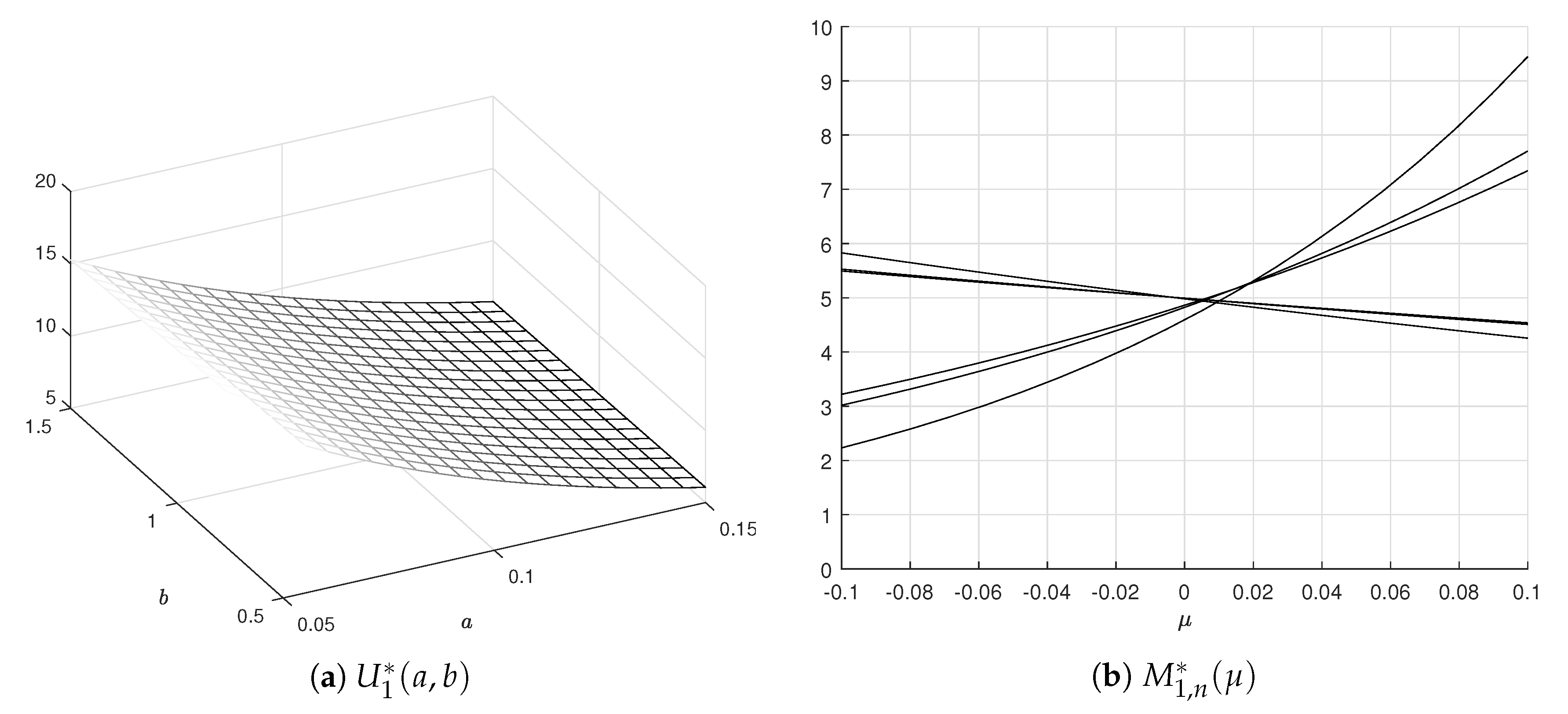
Because the parameters of the $LT$ model are independent, the joint PDFs $U_i^{*}(a,b)=P_i^{*}\left(a\right)F_i^{*}\left(b\right)$ of the parameters and noises have the form

$$\begin{array}{ccc}\hfill U_1^{*}(a,b)& =& 53.09exp(-9.72a)exp\left(0.06b\right),\hfill \\ \hfill U_2^{*}(a,b)& =& 55.49exp(-6.04a)exp\left(0.58b\right),\hfill \\ \hfill U_3^{*}(a,b)& =& 65.81exp(-6.09a)exp(-0.81b),\hfill \end{array}$$

(49)

$$(a,b)\in [0.05,0.15]\bigcup [0.5,1.0],\mu \in [-0.1,0.1],i=\overline{1,24}.$$

Clearly, the PDFs are of exponential type. For $i=1,$ the graphs are shown in Figure 2.

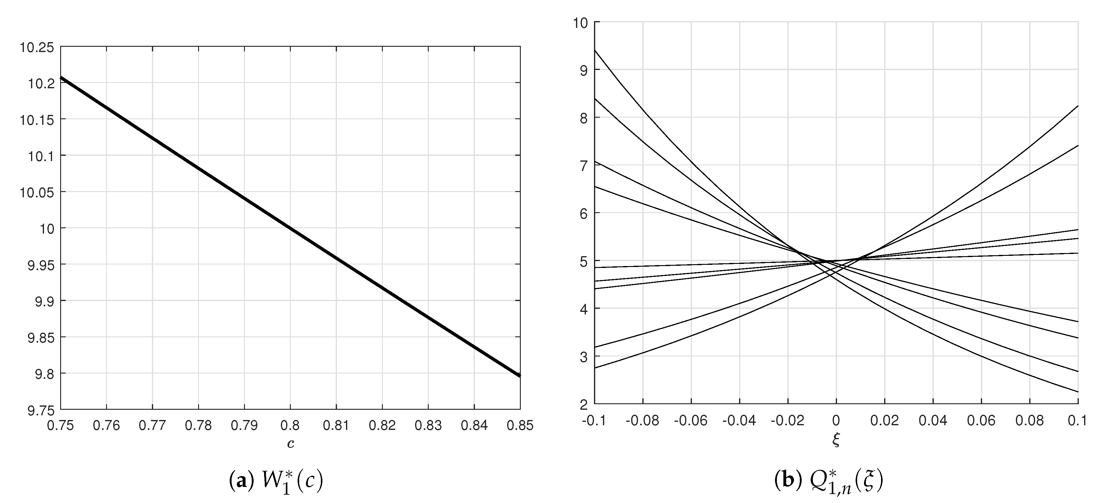
For the $T\xi$ model, the PDFs of the parameters and noises have the form

$$\begin{array}{ccc}\hfill W_1^{*}\left(c\right)& =& 13.90exp(-0.41c),\hfill \\ \hfill W_2^{*}\left(c\right)& =& 10.43exp(-0.05c),\hfill \\ \hfill W_3^{*}\left(c\right)& =& 11.65exp(-0.19c),\hfill \end{array}$$

$$c\in [0.75,0.85],\xi \in [-0.1,0.1],i=\overline{1,24}.$$

For $i=1,$ the graphs can be seen in Figure 3.

Thus, the randomized $LT\xi$ model generates random trajectories with the entropy-optimal PDFs of the model parameters and measurement noises:

$$\begin{array}{ccc}\hfill L\left[n\right]& =& aL[n-1]+bT\left[n\right],\left(P^{*}\left(a\right),F^{*}\left(b\right)\right),\hfill \\ \hfill v\left[n\right]& =& L\left[n\right]+\mu \left[n\right],M_n^{*}\left(\mu \left[n\right]\right);\hfill \\ \hfill \tau \left[n\right]& =& c\left(2.1\tau [n-1]-1.1\tau [n-2]\right),W^{*}\left(c\right),i=\overline{1,3},\hfill \\ \hfill T\left[n\right]& =& t+\tau \left[n\right]+\xi \left[n\right],Q_n^{*}\left(\xi \left[n\right]\right).\hfill \end{array}$$

(50)

The corresponding ensembles are generated by the sampling procedure of the resulting PDFs of the parameters and noises using the acceptance-rejection (AR) method (also known as rejection sampling (RS); see [49]). During calculations, 100 samples for each parameter and 100 samples for each noise were used; in other words, the ensemble consisted of ${10}^4$ trajectories.

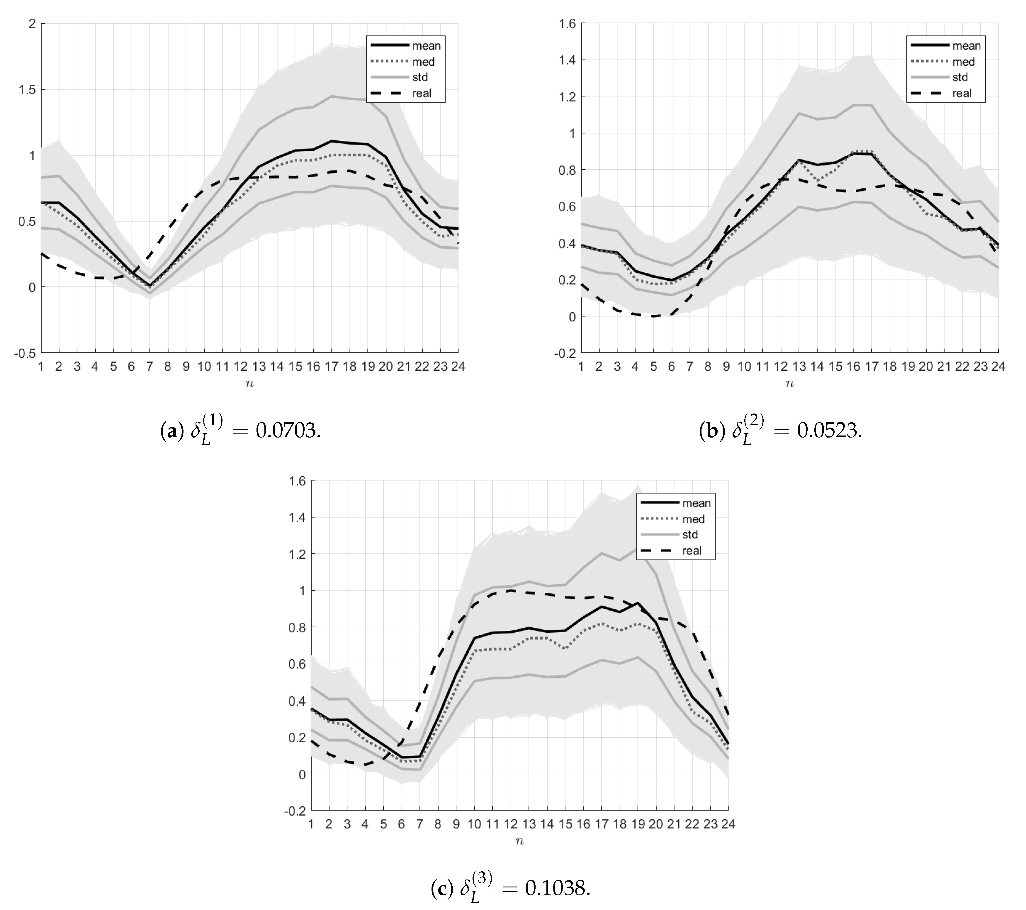
(5). Model Testing.

The adequacy of the model was analyzed by the self- and cross-testing of the $LT$ and $T\xi$ models on the real load–temperature data for 3–5 July 2016 ($i=1,2,3$). Self-testing means generating an ensemble of trajectories with the entropy-optimal parameters and noises for day i, calculating the mean (mean) and median (med) trajectories and also the variance curve (std±) of the ensemble, and comparing the mean trajectory with the real counterparts by electrical load and ambient temperature for the same day i. The quality of approximation is characterized by relative errors,

$${\delta }_L^{\left(i\right)}=\frac{{\displaystyle \sum _{n=1}^{24}}{\left(L_{mean}^{\left(i\right)}\left[n\right]-L_r^{\left(i\right)}\left[n\right]\right)}^2}{{\displaystyle \sum _{n=1}^{24}}{\left(L_{mean}^{\left(i\right)}\left[n\right]\right)}^2+{\displaystyle \sum _{n=1}^{24}}{\left(L_r^{\left(i\right)}\left[n\right]\right)}^2},i=\overline{1,3},$$

(51)

in electrical load and

$${\delta }_T^{\left(i\right)}=\frac{{\displaystyle \sum _{n=1}^{24}}{\left(T_{mean}^{\left(i\right)}\left[n\right]-T_r^{\left(i\right)}\left[n\right]\right)}^2}{{\displaystyle \sum _{n=1}^{24}}{\left(T_{mean}^{\left(i\right)}\left[n\right]\right)}^2+{\displaystyle \sum _{n=1}^{24}}{\left(T_r^{\left(i\right)}\left[n\right]\right)}^2},i=\overline{1,3},$$

(52)

in ambient temperature.

Cross-testing represents a similar procedure in which the mean trajectories are compared with the real counterparts in terms of electrical load and ambient temperature for days $j\ne i.$ The quality of approximation is characterized by relative errors,

$${\delta }_L^{(i,j)}=\frac{{\displaystyle \sum _{n=1}^{24}}{\left(L_{mean}^{\left(i\right)}\left[n\right]-L_r^{\left(j\right)}\left[n\right]\right)}^2}{{\displaystyle \sum _{n=1}^{24}}{\left(L_{mean}^{\left(i\right)}\left[n\right]\right)}^2+{\displaystyle \sum _{n=1}^{24}}{\left(L_r^{\left(j\right)}\left[n\right]\right)}^2},i=\overline{1,3},i\ne j,$$

(53)

in electrical load and

$${\delta }_T^{(i,j)}=\frac{{\displaystyle \sum _{n=1}^{24}}{\left(T_{mean}^{\left(i\right)}\left[n\right]-T_r^{\left(j\right)}\left[n\right]\right)}^2}{{\displaystyle \sum _{n=1}^{24}}{\left(T_{mean}^{\left(i\right)}\left[n\right]\right)}^2+{\displaystyle \sum _{n=1}^{24}}{\left(T_r^{\left(j\right)}\left[n\right]\right)}^2},i=\overline{1,3},i\ne j,$$

(54)

in ambient temperature.

Self-testing. For the $LT$ model, the real ambient temperature data $T_r^{\left(i\right)}\left[n\right]$ as well as the entropy-optimal PDFs $P_i^{*}\left(a\right)$ and $F_i^{*}\left(b\right)$ of the parameters $(a,b)$ and the PDFs $M_1^{*}\left(\mu \left[1\right]\right),\cdots ,M_{24}^{*}\left(\mu \left[24\right]\right)$ of the measurement noises $\mu \left[n\right]$ were used. The ensembles ${\mathbb{L}}^{\left(i\right)}$ were generated using the sampling procedure of the above PDFs. The mean trajectory $L_{mean}^{\left(i\right)}\left[n\right]$, the median trajectory $L_{med}^{\left(i\right)}\left[n\right]$ and also the trajectories $L_{std\pm }^{\left(i\right)}\left[n\right]$ corresponding to the limits of the variance graph were found. The errors ${\delta }_L^{\left(i\right)}$ were calculated. The resulting ensembles and relative errors ${\delta }_L^{\left(i\right)}$ for the three indicated days are demonstrated in Figure 4.

The $T\xi$ model was tested by generating the ensemble ${\mathbb{T}}^{\left(i\right)}$ of random trajectories $T^{\left(i\right)}\left[n\right]$, $n=\overline{1,24}$ with the entropy-optimal PDFs $W^{\left(i\right)}\left(c\right)$ and $Q_1^{*}\left(\xi \left[1\right]\right),\cdots ,Q_{24}^{*}\left(\xi \left[24\right]\right)$ through sampling. The mean trajectory $T_{mean}^{\left(i\right)}\left[n\right]$, the median trajectory $T_{med}^{\left(i\right)}\left[n\right]$ and the trajectory $T_{std\pm }^{\left(i\right)}\left[n\right]$ corresponding to the limits of the variance curve are calculated. The resulting ensembles and relative errors ${\delta }_T^{\left(i\right)}$ for the three days are shown in Figure 5.

Cross-testing. For cross-testing, the $LT$ and $LT\xi$ models learned on the data for day i were used, and their mean trajectories were compared with the data for days $j\ne i$. The resulting errors are combined in

Table 2. Values ${\delta }_L$ obtained by cross-testing of $LT$ model. Mean value ${\delta }_L=0.0530$.

$\mathit{i}/\mathit{j}$	1	2	3
1		0.0495	0.1052
2	0.0858		0.1428
3	0.0569	0.0364

,

Table 3. Values ${\delta }_T$ obtained by cross-testing of $T\xi$ model. Mean value ${\delta }_L=0.0757$.

$\mathit{i}/\mathit{j}$	1	2	3
1		0.1051	0.1079
2	0.1506		0.1185
3	0.1315	0.0676

and

Table 4. Values ${\delta }_T$ obtained by cross-testing of $LT\xi$ model. Mean value ${\delta }_L=0.1478$.

$\mathit{i}/\mathit{j}$	1	2	3
1		0.1437	0.2659
2	0.1756		0.2322
3	0.3475	0.1655

.

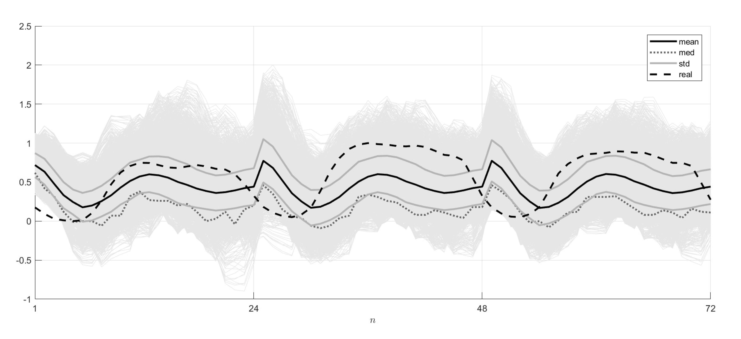
(6). Randomized Prediction of N-Daily Load.

In the randomized prediction of the N-daily load, the $LT\xi$ model learned on the interval ${\mathcal{T}}_l$ was used. The quality of the forecast was characterized using the $LT\xi$ model with the entropy-optimal PDFs obtained on the real data for the first ($i=1$) day.

The 1-day ($n\in [1,24]$), 2-day ($n\in [1,48]$) and 3-day ($n\in [1,72]$) ensembles were constructed by the sampling procedure of the above PDFs. For these ensembles, the mean trajectories $L_{mean}\left[n\right]$, the median trajectories $L_{med}\left[n\right]$ and also the limiting trajectories $L_{std\pm }\left[n\right]$ of the variance curve were found. The forecast results were compared with the real data for 3–7 July 2006 ($i=\overline{1,4}$). The forecasting quality was characterized by the relative errors calculated similar to (53) and (54).

The resulting 24-h, 48-h and 72-h randomized forecasts of electrical load and their probabilistic characteristics (the mean and median trajectories, the limit trajectories of the variance curves) are presented in Figure 6. The errors, i.e., the deviations between the model forecasts and real data, can be seen in

Table 5. Accuracy of 24-h, 48-h and 72-h forecasts using $LT\xi$ model.

${\mathit{\delta }}_{\mathit{L}}^{\left(2\right)}$	${\mathit{\delta }}_{\mathit{L}}^{\left(3\right)}$	${\mathit{\delta }}_{\mathit{L}}^{\left(4\right)}$
0.1509	0.2515	0.2133

.

7. Conclusions

The article proposes a new forecasting approach based on the idea of generation not the only forecast and not a set of forecasts with the scenario’s model parameters, and not forecasts with assigned probabilities, but the ensemble of random forecasts with entropy-optimal model parameters and measurement noises.

For the randomized forecasting we propose a structure of predictive dynamical model which uses as real data as optimized noises. The latter are the source of ensemble of predictive trajectories, which allow computing deterministic trajectories of its different numerical characteristics and probabilistic estimates.