The Study of the Theoretical Size and Node Probability of the Loop Cutset in Bayesian Networks

Abstract

Pearl’s conditioning method is one of the basic algorithms of Bayesian inference, and the loop cutset is crucial for the implementation of conditioning. There are many numerical algorithms for solving the loop cutset, but theoretical research on the characteristics of the loop cutset is lacking. In this paper, theoretical insights into the size and node probability of the loop cutset are obtained based on graph theory and probability theory. It is proven that when the loop cutset in a p-complete graph has a size of $p-2$, the upper bound of the size can be determined by the number of nodes. Furthermore, the probability that a node belongs to the loop cutset is proven to be positively correlated with its degree. Numerical simulations show that the application of the theoretical results can facilitate the prediction and verification of the loop cutset problem. This work is helpful in evaluating the performance of Bayesian networks.

1. Introduction

A Bayesian network is an acyclic, directed graph in which the nodes represent chance variables. The arcs in a Bayesian network represent the probabilistic influences between nodes. An arc implies that it is possible to characterize the relationship between the connected nodes by a conditional probability matrix. Bayesian networks (BNs) play a central role in a wide range of automated reasoning applications. Bayesian inference is a statistical inference method in which Bayes’ theorem is used to update the probability of a hypothesis when additional evidence or information becomes available, and it is an important technique in statistics, especially in mathematical statistics.

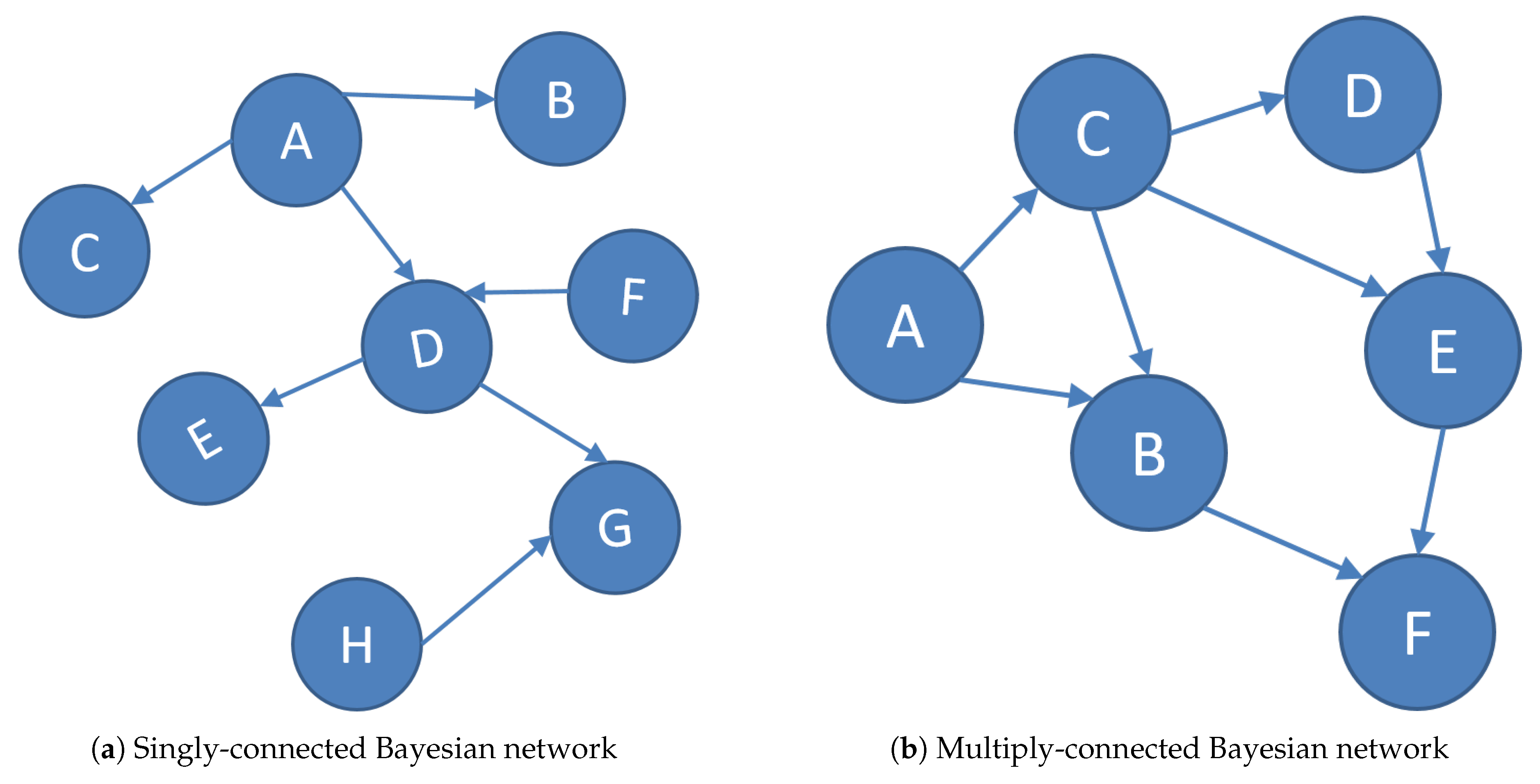
A singly-connected Bayesian network, also known as a causal polytree, has only a single pathway (in the undirected sense) from any node to any other node. A multiply-connected network, on the other hand, can have more than one pathway between nodes.

The conditioning method was proposed by Pearl to solve the inference problem for a multiply-connected Bayesian network, in which the loop cutset is needed to perform conditioning. A loop cutset of a multiply-connected network is a set of nodes (of a specified cardinality) that, if omitted from the graph, results in a singly-connected network. Two examples of singly-connected and multiply-connected Bayesian networks are given in Figure 1. Omitting the node C in the multiply-connected BN can result in a singly-connected BN, then a set of node C is a loop cutset of this BN. The complexity of the conditioning method grows exponentially with the loop cutset size. According to Cooper’s related work, the problem of finding the minimum loop cutset has been proven to be NP-hard [1].

There has been much research on the loop cutset problem, and we review three classes of such algorithms: heuristic algorithms, random algorithms and precise algorithms. The heuristic algorithms are the earliest and most extensively studied among these three types of algorithms, and the greedy algorithm plays an important role in heuristic algorithms. One of the most typical greedy algorithms was proposed by Suermondt and Cooper in 1988 [2,3]. Becker and Geiger proposed the modified greedy algorithm (MGA) [4] for finding the loop cutset in 1996, and then Becker proposed a random algorithm called the weighted randomized algorithm (WRA) [5] for solving the loop cutset problem in 1997. Based on existing accurate algorithms for the feedback vertex set (FVS) problem, the complexity of the precise algorithm for the loop cutset problem can be restricted to $0\left({1.7548}^n\right)$ [6].

However, in contrast to the abundance of numerical algorithms for solving the loop cutset in the present literature, theoretical research on the characteristics of the loop cutset is lacking; thus, the algorithms lack theoretical support. In the heuristic algorithm, the node with the highest degree (i.e., the number of edges connected to the node) is supposed to be the first node of the loop cutset by default. In the random algorithm WRA, the node is picked at the random with probability $deg\left(v_i\right)/{\sum }_{u\in V_i}deg\left(u\right)$ where $v_i$ and u are the nodes in graph $G_i\left(V_i,E_i\right)$, and $deg\left(v_i\right)$ is the degree of node $v_i$. Then, why can the node with the highest degree become a candidate for the loop cutset? Is it possible to perform some preanalysis on the loop cutset before solving? Importantly, performing preanalysis to evaluate the existence of cutsets and the size of the loop cutset can reduce unnecessary calculations in some cases.

Based on the above considerations, in this paper, the size and node-probability of the loop cutset are analyzed. We derive the relevant theorem for predicting the size of the loop cutset based on loop theory in graph theory. Much research has focused on loops in graph theory because, in real scenarios, loops must often be broken. The loop cutset is based on similar requirements. The introduction of the loop cutset in the BNs also breaks the loop and avoids shock and instability during the message transmission process. Related theoretical work on the node-probability of the loop cutset is conducted to provide theoretical support for the conditions of the heuristic algorithm.

In some studies, the ratio $C/V$ between the number of leaf nodes C and the number of root nodes V is proposed to measure the growth of a clique tree (i.e., a mapping of a graph into a tree that can be used to define the treewidth of the graph and speed up solving certain computational problems on the graph), in bipartite BNs. Inspired by this, the indicator $r_{-}deg\left(v\right)$ is proposed in this paper to measure the relative size of the node degree, and is related to the node probability of the loop cutset through experimental analyses.

The rest of the paper is organized as follows. Section 2 provides some preliminary knowledge and introduces the loop cutset problem. In Section 3, we perform some theoretical analyses of the loop cutset, predict the theoretical size of the loop cutset, and analyze the theoretical probability that a node belongs to the loop cutset. Section 4 programs and performs data experiments on four existing algorithms, and the results verify the correctness of the relevant theories.

2. Preliminaries

Definition 1.

(graph concepts) A directed graph is a pair $\mathrm{D}=\langle V,E\rangle$, where $\mathrm{V}=\left\{X_1,\dots ,X_n\right\}$ is a set of nodes and $\mathrm{E}=\left\{\left(X_i,X_j\right)|X_i,X_j\in V\right\}$ is the set of edges. Given $\left(X_i,X_j\right)\in E$, $X_i$ is called a parent of $X_j$, and $X_j$ is called a child of $X_i$. The moral graph of a directed graph D is the undirected graph obtained by connecting the parents of all the nodes in D and removing edge orientation. A cycle cutset of an undirected graph is a subset of nodes that, when removed, yields a graph without cycles. A loop in a directed graph D is a subgraph of D in which the underlying graph is a cycle. A directed graph is acyclic if it has no directed loops. A directed graph is singly connected (also called a poly-tree), if its underlying undirected graph has no cycles; otherwise, it is called multiply connected. A complete graph is a simple undirected graph in which every pair of distinct vertices is connected by a unique edge. A p-complete graph is a complete graph with p nodes [7].

Definition 2.

(loop cutset) A vertex v is a sink with respect to a loop L if the two edges adjacent to v in L are directed into v. A vertex that is not a sink with respect to a loop L is called an allowed vertex with respect to L. A loop cutset of a directed graph D is a set of vertices that contains at least one allowed vertex with respect to each loop in D [7].

Definition 3.

(Bayesian Networks) Let $\mathrm{X}=\left\{X_1,\dots ,X_n\right\}$ be a set of random variables over multivalued domains $\mathcal{D}\left(X_1\right),\dots ,\mathcal{D}\left(X_n\right)$. A BN (Pearl, 1988), which is also named a belief network, is a pair $<G,P>$ where G is a directed acyclic graph in which nodes are the variables X, and $P=\left\{P\left(X_i|p{a}_i\right)|i=1,2,\dots ,n\right\}$ is the set of conditional probability tables (CPTs) associated with each $X_i$. The BN represents a joint probability distribution having the product form:

$$\mathrm{P}\left(x_1,\dots ,x_n\right)=\prod _{i=1}^{n}P\left(x_i|pa\left(X_i\right)\right)$$

Evidence e is an instantiated subset of variables $\mathrm{E}\subset \mathrm{X}$ [7].

Loop Cutset Problem:

Conditions: Directed acyclic graph $G=(V,E)$, integer k.

Goal: Find a set $S\subseteq V$ such that $\left|S\right|\le k$ and $G^{\prime }$ is a forest (i.e., an undirected acyclic graph all of those in which the connected components are trees), where $G^{\prime }=\left(V,E^{\prime }\right),E^{\prime }=\{(u,v)\in E,u\notin S,v\notin S\}$.

The loop cutset problem can be transformed into an FVS problem as follows: convert the directed acyclic graph $G=(V,E)$ to its underlying graph. Then, iteratively delete the nodes of which degrees are less than 2 and delete the adjacent edges, and finally a new undirected graph is obtained. Denote the undirected graph obtained as $G_{new}=\left(V_{new},E_{new}\right)$. Now, the problem involves finding a loop cutset $\mathrm{S}\subseteq V_{new}$ for $G_{new}=\left(V_{new},E_{new}\right)$.

3. The Theoretical Size and Node Probability of the Loop Cutset

In this section, some theoretical work has been done on the loop cutset: denoting the loop cutset as S and the size of S as $\left|S\right|$, we give several theorems and related inferences regarding the upper and lower bounds of $\left|S\right|$ and the probability of a node belonging to S.

These theories on the upper and lower bounds of $\left|S\right|$ are based on the loop theorem in graph theory. A significant amount of research on loops in graph theory has been done because it is important to break the loops in a graph in practical applications. The loop cutsets break loops in BNs so that unstable effects will not be produced in the message-passing process. Little previous theoretical research has been done on this aspect of the loop cutset. Research on these issues can provide a basis for predicting the size of the loop cutset, verifying the results, and analyzing the BNs in advance.

The conclusion that “the greater the degree of a node, the greater the probability that the node belongs to the loop cutset” was used directly when Suermondt and Cooper proposed a heuristic algorithm, although without any theoretical basis. In this section, this conclusion is proven to build a theoretical foundation for the heuristic algorithm. Based on graph theory, several theorems and corollaries about the upper and lower bounds of $\left|S\right|$ and the probability that a node belongs to S are given below.

3.1. Upper and Lower Bounds of $\left|S\right|$

Theorem 1.

If the undirected graph $G=(V,E)$ is a p-complete graph $K_p$, then $\left|S\right|=p-2$.

Proof of Theorem 1.

The theorem is proven via mathematical induction.

For a 3-complete graph $K_3$, it can be clearly concluded that $\left|S\right|=1=p-2$, where $p=3$ for the 3-complete graph.

Let the conclusion hold when $p=k$. Next, it will be proven that the conclusion holds when $p=k+1$.

For a $(k+1)$-complete graph $K_{(k+1)}$, remove any $(k-2)$ nodes and then there are three nodes left in the graph. By the definition of a complete graph, these three nodes are connected to form a circle. Therefore, we now need to remove one node to form a forest. Thus, the size of the loop cutset $\left|S\right|=k-1=p-2$. □

Corollary 1.

For any undirected graph $G=(V,E)$, $\left|S\right|\le p-2$, where p is the number of nodes in the graph.

Proof. 

The conclusion can be drawn in conjunction with Theorem 1, according to the definition of a complete graph. □

Theorem 2.

For an undirected graph $G=(V,E)$, if for all nodes, the degree is even and greater than 0, then $\left|S\right|\ge 1$.

Proof of Theorem 2.

This theorem is proven by using the longest path method.

Let the longest path $v_1{v}_2{v}_3\dots v_n$ in the graph be denoted as $l_{max}$ and its length as n.

From the given conditions, it can be concluded that $deg{v}_1\ge 2$. Then, there is at least one node adjacent to $v_1$ in addition to $v_2$, denoting this adjacent node as $v_{1_2}$.

If $v_{1_2}$ is not on the longest path $l_{max}$, then there is a path $v_{1_2}{v}_1{v}_2{v}_3\dots v_n$ in the graph in which the length is $(n+1)$, which conflicts with the longest path assumption. Thus, $v_{1_2}$ is on the longest path $l_{max}$; that is,

$$\exists v_i,3\le i\le n,s.t.v_1{v}_i\in E$$

Thus, $v_1{v}_2\cdots v_i{v}_1$ is a loop, and $v_i$ can be put into the loop cutset as a loop cut vertex, that is, $\left|S\right|\ge 1$. □

Theorem 3.

For an undirected graph $G=(V,E)$, denote the minimum degree of all nodes in the graph as $\delta \left(G\right)$. If $\delta \left(G\right)\ge 2$, then $\left|S\right|\ge 1$; if $\delta \left(G\right)\ge m\ge 2$, then $\left|S\right|\ge m-1$.

Proof of Theorem 3.

This theorem is proven by using the longest path method.

(1)

The first part of the theorem can be derived from Theorem 2 directly.

(2)

Similar to the proof of Theorem 2, the longest path method can also be used to prove this theorem. Let the longest path $v_1{v}_2{v}_3\dots v_n$ in the graph be denoted as $l_{max}$ and its length as n.

From the known conditions, it can be concluded that $deg{v}_1\ge m$. Then, there are at least m-1 nodes adjacent to $v_1$ in addition to $v_2$, and denote these adjacent nodes as $v_{1_i},i=1,\dots ,m-1$.

If $v_{1_j}$ is not on the longest path $l_{max}$, then there is a path $v_{1j}{v}_1{v}_2{v}_3\dots v_n$ in the graph in which the length is $n+1$, which conflicts with the longest path assumption.

Thus, each node adjacent to $v_1$ is on the longest path $l_{max}$. Then, there are $m-1$ different loops with m-1 different loop cut vertices. That is, $\left|S\right|\ge m-1$. □

3.2. The Node Probability of the Loop Cutset

Theorem 4.

For an undirected graph $G=(V,E)$ with all nodes of degree greater than 2, the probability that node v belongs to the loop cutset satisfies the following relationship:

$$p(v\in S)\ge 1-{\left(1-\frac{degv·(degv-1)}{(n_{nodes}-1)(n_{nodes}-1)}\right)}^{(n_{edges}-degv)}$$

where $n_{nodes}$ and $n_{edges}$ are the numbers of nodes and edges, respectively.

Proof of Theorem 4.

Node v divides graph G into two graphs $G_1$ and $G_2$, where $G_1=\left(V_1,E_1\right)$, $V_1=\left\{v\right\}\cup \left\{\widehat{v}\right|\widehat{v}\in V,\exists (\widehat{v},v)\in E\}$, $E_1=\left\{(v,u)\right|(v,u)\in E\}$, and $G_2=G\setminus G_1$.

Taking $G_1$ as the initial graph, add the edges from $G_2$ one by one to $G_1$. Here, assume that the endpoint of each edge is selected from V with moderate probability. Consider the probability of forming a loop containing v (we hereafter refer to this type of loop as a v-loop ).

Consider the case in which the length of the v-loop is 3.

While adding edges one by one, there is at least one edge $(u,w)$ such that both of its endpoints belong to $V_1$, $\mathrm{u},\mathrm{w}\in V_1$. The probability of this situation is calculated as follows:

$$\begin{array}{c}\hfill p(v-\mathrm{loop}\mathrm{exist}\&\mathrm{length}=3)\\ \ge 1-{\left(1-\frac{degv·(degv-1)}{(n_{nodes}-1)(n_{nodes}-1)}\right)}^{(n_{edges}-degv)}\hfill \end{array}$$

The above inequality is an equality only when all edges in $G_2$ include a node that shares an edge with v.

Thus,

$$\begin{array}{cc}\hfill p(v-\mathrm{loop}\mathrm{exist})& \hfill \\ \hfill & \ge p(v-\mathrm{loop}\mathrm{exist}\&\mathrm{length}=3)\hfill \\ \hfill & \ge 1-{\left(1-\frac{degv·(degv-1)}{(n_{nodes}-1)(n_{nodes}-1)}\right)}^{(n_{edges}-degv)}\hfill \end{array}$$

 □

Corollary 2.

For an undirected graph $G=(V,E)$ with all nodes of degree greater than 2, the probability that node u belongs to the loop cutset is related to the degree of the node. The greater the degree of the node is, the greater the probability.

Proof. 

This corollary can be derived from Theorem 4. □

4. Experiments

In this section, four existing algorithms are implemented: the greedy algorithm $A_1$ [2,3] proposed by Suermondt and Cooper, the improved algorithm $A_2$ [8] for $A_1$ proposed by Stillman, the MGA [4] proposed by Becker and Geiger, and the WRA [5] proposed by Becker. A large number of random BNs are randomly generated and applied with the above four algorithms. The experimental results of the four existing algorithms are compared, and the overall influence trend of the numbers of nodes and edges on loop cutset size is analyzed using a new parameter, which is related to the number of nodes and edges. Finally, the influence of the degree on the node probability of the loop cutset is studied to verify the theory proposed in Section 3.

It should be pointed out that in the WRA algorithm, the user needs to specify two constants c and Max. The constant c is related to the correct probability of the algorithm result, and the constant Max is related to the solution speed. Referring to [5], we take the value of c as 1, and the value of Max as 300 here.

Seven groups of BNs are randomly generated by using the algorithm in reference [3]. The generation parameters are the number of nodes, the number of edges, and the value range of the nodes (corresponding to $\left|V\right|$, $\left|E\right|$, and values in

Table 1. The random graphs generated by different parameters and the results of four algorithms.

	$\left|\mathit{V}\right|$	$\left|\mathit{E}\right|$	Values	t(${\mathit{A}}_1$)	t(${\mathit{A}}_2$)	t(MGA)	t(WRA)	sz(${\mathit{A}}_1$)	sz(${\mathit{A}}_2$)	sz(MGA)	sz(WRA)
$G1$	15	25	2–6	0.0172	0.0162	0.0609	9.090	3.77	3.77	3.01	4.30
$G2$	15	25	2–8	0.0158	0.0159	0.0586	9.042	3.81	3.83	2.87	4.37
$G3$	15	25	2–10	0.0158	0.0160	0.0594	9.112	3.78	3.82	2.87	4.38
$G4$	25	55	2–6	0.0298	0.0295	0.1277	17.18	7.47	7.41	5.76	8.53
$G5$	25	55	2–8	0.0297	0.0295	0.1272	17.19	7.4	7.39	5.73	8.63
$G6$	25	55	2–10	0.0297	0.0294	0.1283	17.17	7.37	7.35	5.87	8.72
$G7$	55	125	2–10	0.0781	0.0798	0.3918	45.20	14.19	14.22	11.40	17.20

, respectively). The experiments compare the results of $A_1$, $A_2$, MGA and WRA based on these randomly generated graphs as shown in Table 1. The data of the results compared in Table 1 are the time taken by four algorithms (in seconds) and the mean cardinality of the loop cutset in the corresponding experimental group.

$A_2$ is the improved version algorithm of $A_1$, and the difference between the two in actual performance is very small according to Table 1. However, in the effort to find the smallest loop cutset, MGA obviously goes further. MGA takes little time, and its loop cutset is small. WRA has the greatest complexity and consumes the most time (for $c=1,Max=300$); additionally, the advantage of the algorithm’s results is not obvious from the mean size.

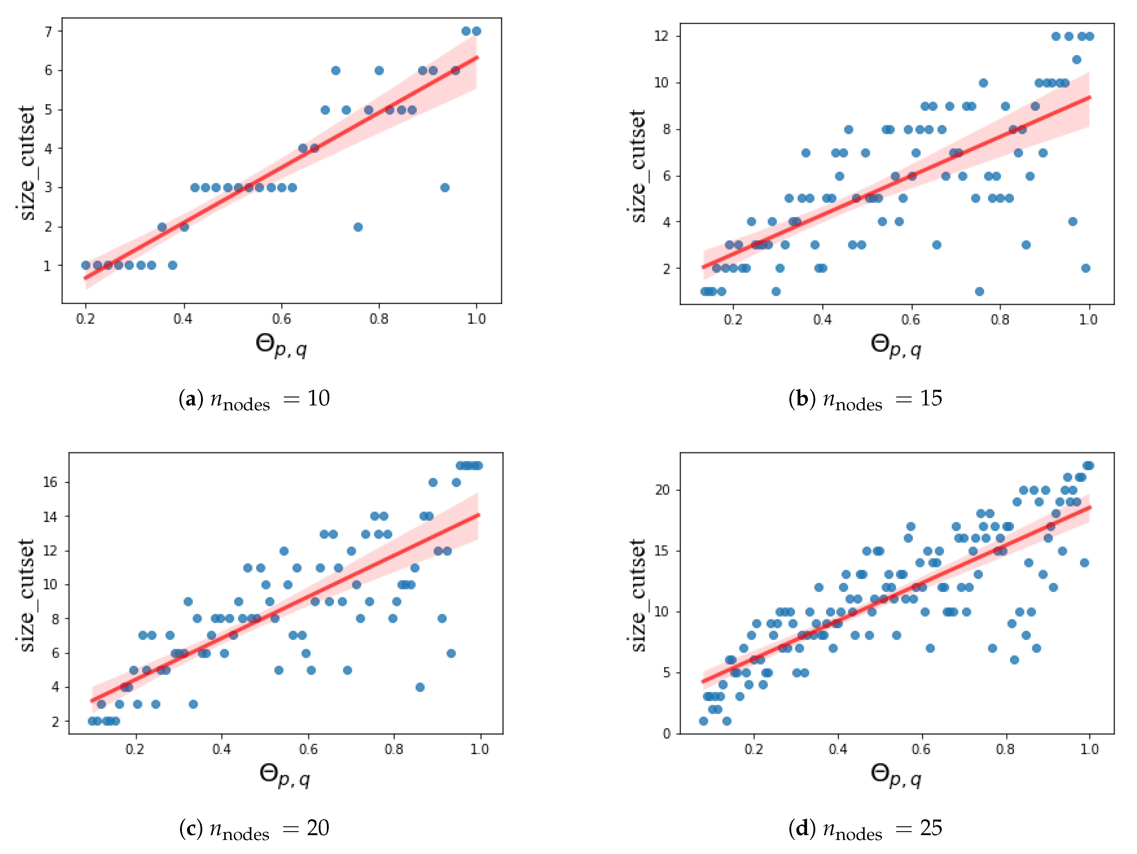
Considering the influence of the numbers of nodes and edges on the size of the loop cutset, it can be seen from Table 1 that as the numbers increase, the size of the loop cutset also increases. Next, by keeping the number of nodes unchanged, changing the number of edges, and using the MGA algorithm to solve the cutset, a new trend is obtained in Figure 2, where a new parameter, related to the number of nodes and edges, is used.

A graph that contains neither parallel edges nor self-loops is called a simple graph. For a simple graph $G=(V,E)$, denote the number of nodes as p, and the number of edges as q, where p and q satisfy the relationship $\mathrm{q}\le \frac{1}{2}p(p-1)$ naturally. We define a new parameter ${\mathsf{\Theta }}_{p,q}$ and let ${\mathsf{\Theta }}_{p,q}=2q/p(p-1)$. The range of ${\mathsf{\Theta }}_{p,q}$ is [0,1].

The change trend of the loop cutset size with the parameter ${\mathsf{\Theta }}_{p,q}$ is given in Figure 2. The size increases as ${\mathsf{\Theta }}_{p,q}$ increases, and the trend is approximately linear. According to the definition, ${\mathsf{\Theta }}_{p,q}$ can be considered as an index reflecting the complexity of graphs.

The relationship between the loop cutset and numbers of nodes and edges is studied above from the global perspective of the graph. Next, from the perspective of each node, the influence of the degree of a node on the node-probability of the loop cutset is studied.

Denote the largest node degree in Graph G as $\mathsf{\Delta }\left(G\right)$, the degree of node v as $deg\left(v\right)$, and the ratio $deg\left(v\right)/\mathsf{\Delta }\left(G\right)$ as $r_{-}deg\left(v\right)$. In Figure 3, $r_{-}deg\left(v\right)$ is used as an independent variable. When $r_{-}deg\left(v\right)=1$, node v has the highest degree in G. Here, the relationship between $r_{-}deg\left(v\right)$ and the probability that the node belongs to the loop cutset is studied.

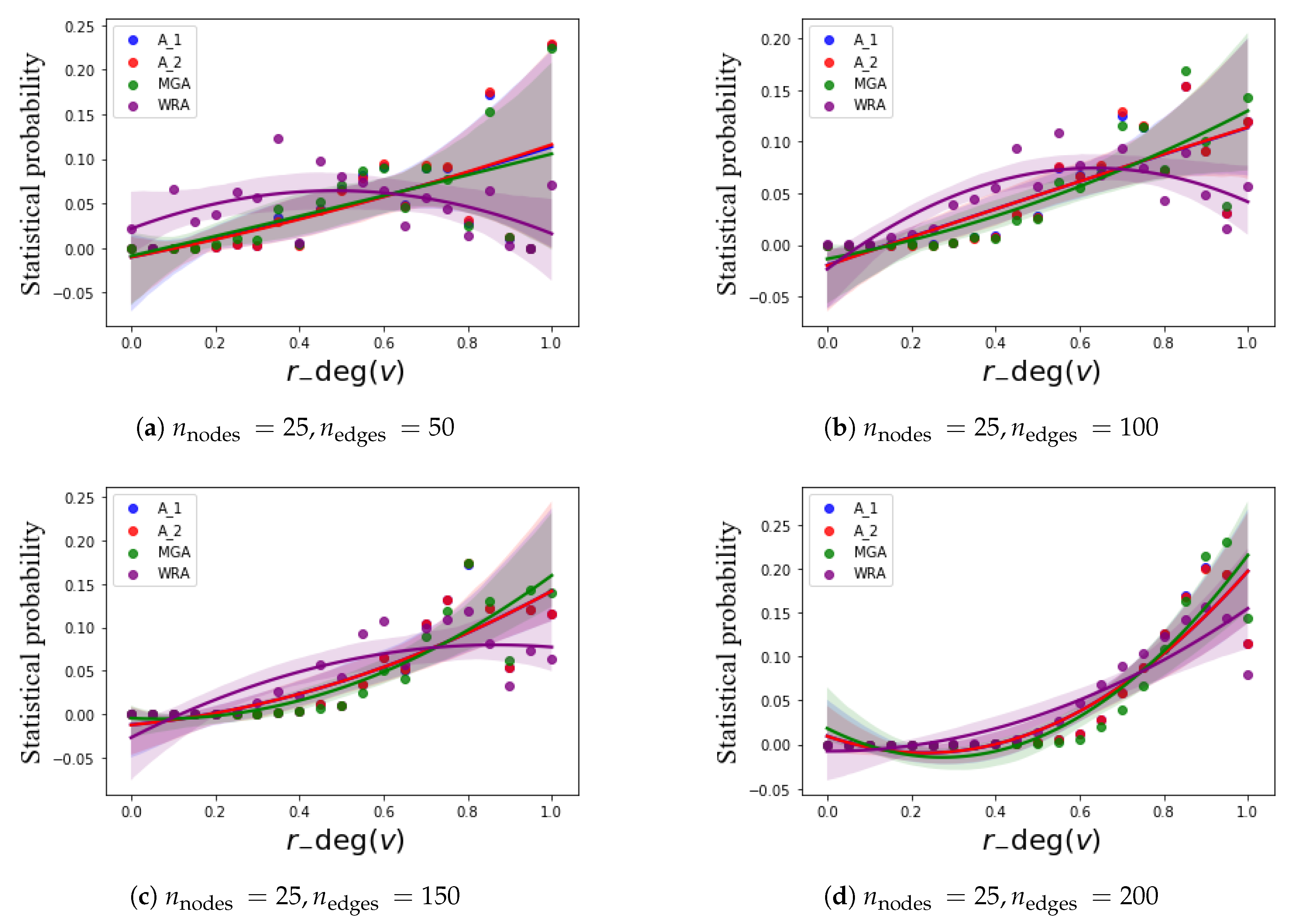
We have implemented the following experiment: four groups of BNs, in which the number of nodes is 25 and the numbers of edges are 50, 100, 150, 200, respectively, are randomly generated and applied with the four algorithms. The number of BNs in each group is 500. The experimental results are compared, and shown in Figure 3. In Figure 3, the x axis is the $r_{-}deg\left(v\right)$ of the node, and the y axis is the statistical node probability belonging to the cutset. According to the results in Figure 3, it can be easily obtained that the statistical node probability increases with the increase of $r_{-}deg\left(v\right)$, and this trend is more obvious when the graph is more complicated (with a greater number of edges).

The statistical probability of $r_{-}deg\left(v\right)$ between 0.9 and 1 has dropped significantly, which needs to be discussed. We tend to a possibility that the largest-degree node and the next-largest in a graph have a very high probability of being adjacent. According to the definition and solution operation of the loop cutset, every node in the loop cutset and its adjacent edges need to be removed. Then iteratively remove the nodes and adjacent edges of which the degree is 1 in the remaining graph. If the two nodes with the highest degree and the next-largest degree are adjacent and share multiple edges, the possibility of the next-largest node in the loop cutset will become smaller when the node with the largest degree is selected into the loop cutset, because it may have been deleted or at least its degree has become smaller.

From the experiments, it can be concluded that the theory obtained in Section 3 is consistent with the experiments; that is, the node degree is positively correlated with the node probability of the loop cutset. In addition, the parameter $r_{-}deg\left(v\right)$ is defined to measure the relative size of the node degree in the graph.

5. Conclusions

The experimental results verify the correctness of the theoretical analyses. For some specific graphs, such as complete graphs, the size of the loop cutset can be obtained directly. For general graphs, the range of the loop cutset size can be derived by the range of node degrees. This range can be used not only to verify the validity of some problems, such as when the required size is so small that it is not in this range, but also to verify the correctness of the results. Some invalid operations can be reduced in actual operations. The complexity of BNs can be evaluated by the size of the loop cutset. In addition, a new indicator $r_{-}deg\left(v\right)$ is defined to measure the relative size of the node degree in the graph.

Finally, we would like to discuss potential future research with the loop cutset based on our theoretical analyses. First, as a key indicator of BNs, the loop cutset can be studied regarding its contribution to the BN structure and its impact on the difficulty of the Bayesian inference. Second, since the node degree has such a direct impact on the node probability, it is an issue whether the loop cutset can be obtained directly according to the node degree in some specific BNs. Third, the largest-degree node and the next-largest node in a graph can be studied to find if they have some relationship, especially the probability of sharing adjacent edges and nodes.