Self-Similar Models: Relationship between the Diffusion Entropy Analysis, Detrended Fluctuation Analysis and Lévy Models

Abstract

Financial and geophysical data, like many other low and high frequency time series, are known to exhibit some memory effects. These memory effects may be long or short, permanent or temporal depending on the event that is being modeled. The purpose of this study is to investigate the memory effects characterized by the financial market closing values and volcanic eruption time series as well as to investigate the relation between the self-similar models used and the Lévy process. This paper uses highly effective scaling methods including Lévy processes, Detrended Fluctuation Analysis (DFA) and Diffusion Entropy Analysis (DEA) to examine long-range persistence behavior in time series by estimating their respective parameters. We use the parameter of the Lévy process (α) characterizing the data and the scaling parameters of DFA (H) and DEA (δ) characterizing the self-similar property to generate a relationship between the three (3) aforementioned scaling methods. Findings from the numerical simulations confirm the existence of long-range persistence (long-memory behavior) in both the financial and geophysical time series. Furthermore, the numerical results from this study indicates an approximate inverse relationship between the parameter of the Lévy process and the scaling parameters of the DFA and DEA (i.e., $H,\delta \approx \frac{1}{\alpha }$), which we prove analytically.

1. Introduction

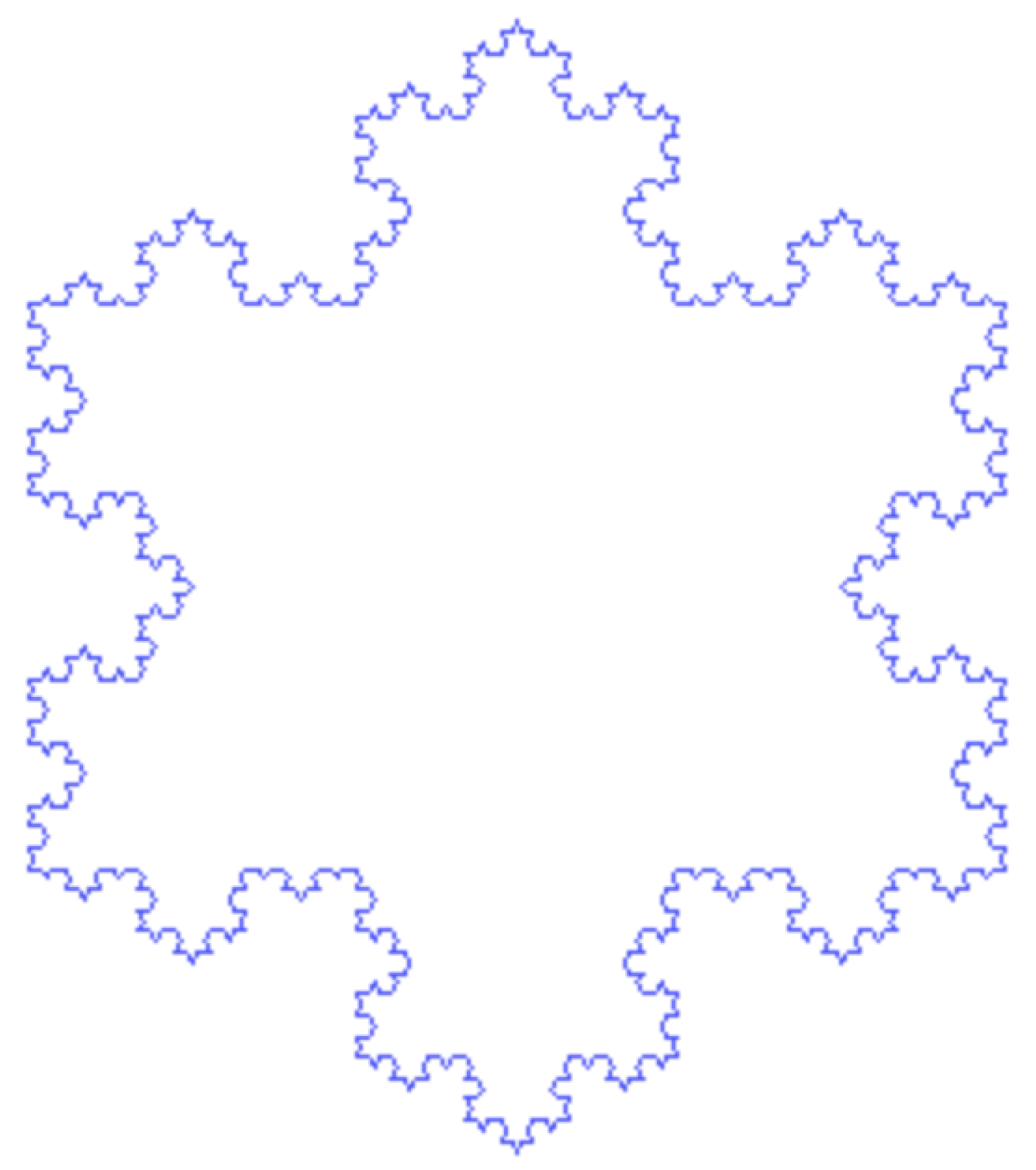
In recent years, researchers have developed several techniques to predict and forecast real-world events or processes that are seemingly difficult to predict due to their complex nature. Such studies have produced major improvements in predictions related to financial market crashes, volcanic activities, climates, heartbeats, etc. Mandelbrot (1982), in the article “The Fractal Geometry of Nature”, describes the surprisingly excellent resemblance between real landscapes and geometrically generated landscapes using simple fractal models [1]. He pointed out that fractals can exhibit self-similarity in enormous ways. A small portion of snowflake depicts similar statistical properties as the whole: a simple example of a self-similar process. This is illustrated by the Koch snowflake curve shown in Figure 1.

Self-similar processes are used to describe stochastic processes that exhibit the phenomenon of self-similarity. These processes occur in several areas of applied mathematics such as fractals, chaos theory, long-memory processes and spectral analysis. That a self-similar process exhibit long-memory effects implies the dependence in time series decays more slowly than an exponential decay, represented as a power-law relation. Let us now take a look at the formal definition of a self-similar process.

Definition 1

(Self-Similarity).In the sense of finite dimensional distributions $\left(\stackrel{fdd}{=}\right)$, we define a stochastic process $X_t$ as self-similar if two processes ${\left\{X_{at}\right\}}_{t\ge 0}$ and ${\left\{a^H{X}_t\right\}}_{t\ge 0}$ have the same law if there exists $\mathit{H}>0$. i.e.,

$${\left\{X_{at}\right\}}_{t\ge 0}\stackrel{fdd}{=}{\left\{a^H{X}_t\right\}}_{t\ge 0}$$

(1)

where $a>0$ is a scale factor and H is the self-similar parameter of the stochastic process $X_t$ [2].

The variances of financial market indices and seismic energy released from volcanic eruptions are stochastic. They are time-varying and they rise during high fluctuation periods. The self-similar properties exhibited by such events are determined by estimating the trends in smaller windows of time over the entire series. This method, known as the Detrended Fluctuation Analysis (DFA), was developed by Peng et al. in the paper “Mosaic Organization of DNA Nucleotides” [3]. The DFA converts a series into a random walk and uses least squares to estimate trends and fluctuations [4,5]. This technique is capable of detecting long-range persistence (self-similar pattern) in both stationary and non-stationary time series.

An alternative to the DFA technique is the Diffusion Entropy Analysis (DEA) model developed by Scafetta et al. (2002), also called a pdf-scaling method. The DEA can be used to investigate if a time series is characterized by Gaussian or Lévy distribution [6,7]. It also permits the detection of long-range persistence in time series. Scafetta (2003) argues that the DEA is the only method that correctly quantifies the self-similarity parameter of time series of complex processes [6].

Researchers have applied these models to diverse fields including DNA sequences [8,9,10], neural oscillations [11], speech pathology detection [12], and heartbeat fluctuation in different sleep stages [13]. The suite of models offered by Peng (1994) and Scafetta (2002) prove to be some of the best techniques for detecting long-range persistence in stationary and non-stationary time series.

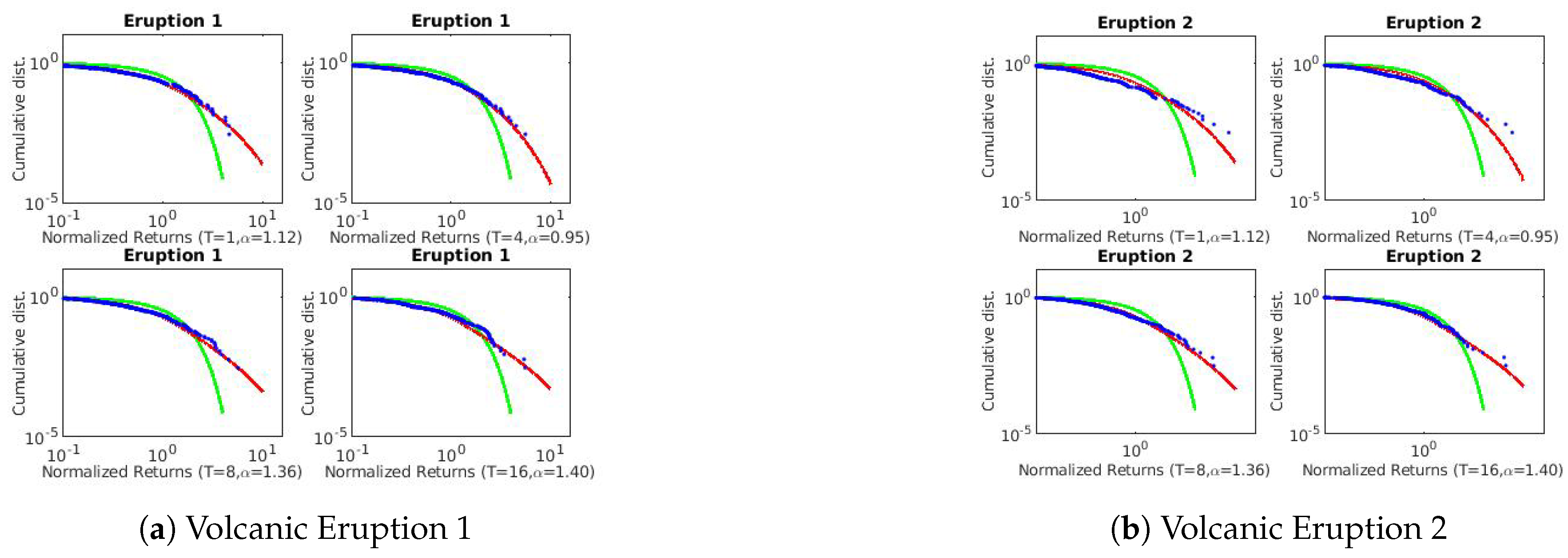
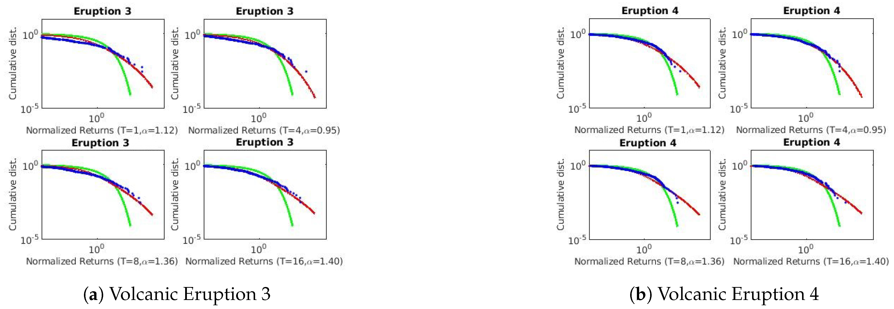
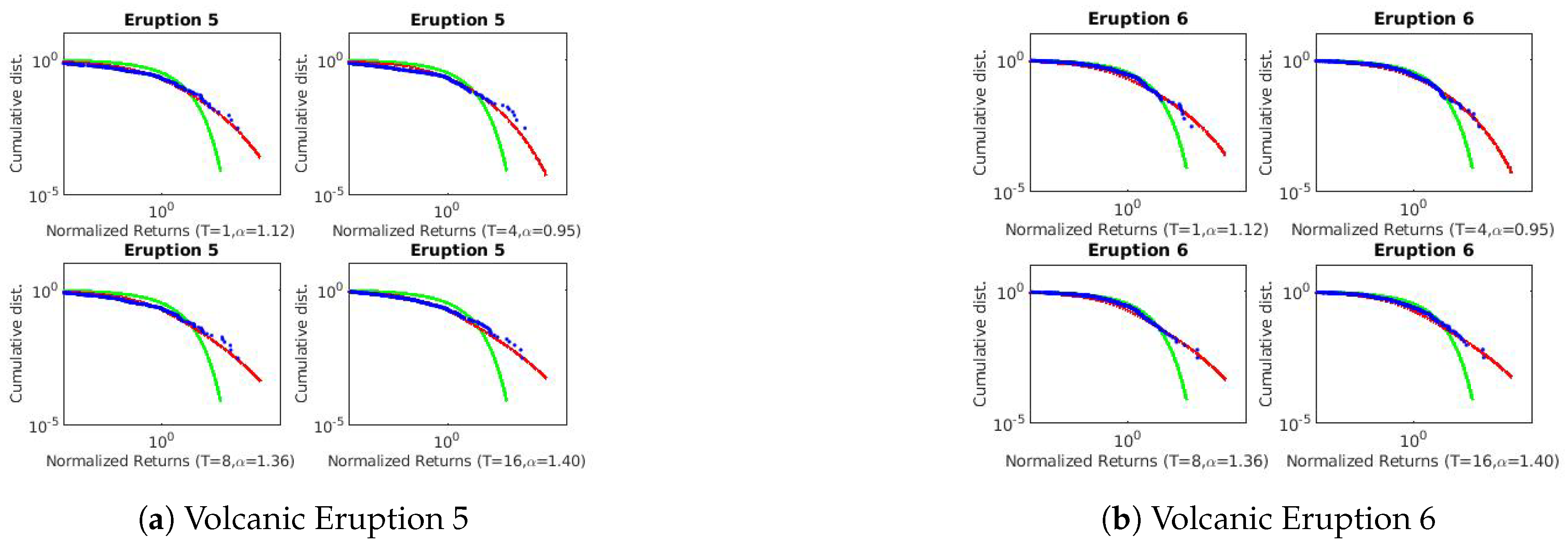
Unlike non-Gaussian Lévy processes that perform poorly in long-range correlation scales, Lévy flights have been used to model evolution of complex stochastic events [14,15,16]. The Lévy flight is a stochastic process that is based on the random succession of steps on space (random walk theory) and probability distribution of the step-sizes which are known to have heavy-tails. In particular, Lévy flights characterizes random steps on a discrete space while Lévy walk describes random steps on a continuous space. However, researchers use “Lévy flights” to describe both cases in literature sometimes [17,18]. Lévy flights have been used to model several events including financial market crashes and trajectories followed by animals when they hunt for food [19,20,21], etc. This is as a result of the generalized central limit theorem (GCLT). When a large collection of step-sizes of a random trajectory satisfy the power-law condition, the Lévy flight distribution is stable: the reason for choosing the Lévy flight distribution to characterize the financial and geophysical processes exhibited by the real-world time series used herein.

In the paper “detecting market crashes by analyzing long memory effects using high-frequency data” by Barany et al. (2012), the authors estimated long-memory behavior in high-frequency financial time series using the DFA, Rescaled-Range Analysis (R/S) and the Lévy flight model to detect market crashes. They go further to generate an inverse relationship between the Hurst exponent and the Lévy model parameter. This close relationship proposes a satisfactory self-similar pattern for analysis [2].

In this paper, we generate a numerical relationship between the Lévy parameter α characterizing the data and the resulting parameters $(H,and\delta )$ of the DFA and DEA characterizing the self-similar property respectively. Furthermore, we prove analytically the relationship obtained. To perform these tasks, we first investigate the existence of long-range persistence in sets of financial market indices and recordings of volcanic eruptions using the DFA, DEA. We report on the scaling parameters of the DFA and DEA and conclude that the time series exhibits long-range correlation (or long-range persistence) if $0.5<H,\delta <1$, and anti-persistent if $0<H,\delta <0.5$. Useful tables of results and plots of the fitted models are reported.

The outline of this paper is as follows. Section 2 details the scaling methods and description of the real-world data used in this paper. Section 3 contains the numerical results and proposed relationships as well as proofs. Section 4 provides a detailed discussion of the results. Section 5 concludes. Some proofs, figures and plots generated from our numerical simulations are provided in the Appendix.

2. Methods

In this section, we describe three techniques for estimating self-similarity or long-range correlations in time series. There are several methods used to estimate scaling exponents of time series to investigate long-memory behavior. In this study, we limit ourselves to Lévy flight model, DFA and DEA techniques for quantifying self-similarity. Note that $\alpha ,H,\delta$ are used to denote the Lévy, DFA and DEA scaling exponents respectively. An overview of the real-world data used for the purpose of evaluating and comparing these three scaling methods are also described.

2.1. Lévy Flight Model

The stable Lévy process (Lévy flight model) has independent increments but are designated as long memory processes [2]. Lévy et al. [22] discovered that the most general representation of a stable distribution is through the characteristic functions $\phi \left(q\right)$. These characteristic functions are defined as:

$$ln\left(\phi \left(q\right)\right)=\mu q-\gamma \mid q\mid \left[1+i\beta \frac{q}{\mid q\mid }\frac{2}{\pi }log\left(q\right)\right],if\alpha =1$$

(2)

and

$$ln\left(\phi \left(q\right)\right)=i\mu q-\gamma \mid q{\mid }^{\alpha }\left[1-i\beta \frac{q}{\mid q\mid }tan\left(\frac{\pi \alpha }{2}\right)\right],if\alpha \ne 1$$

(3)

where the scaling parameter of the Lévy: $0<\alpha \le 2$, $\gamma$ is a positive scale factor (${\gamma }^2$ = ${\sigma }^2$(variance)), $\mu$ is a real-valued constant known as the location parameter (or mean) and $-1\le \beta \le 1$ is the skewness parameter.

Analytically, the stable Lévy distribution is only known for a few values of $\alpha$ and $\beta$. Consider the centered symmetric distribution ($\beta =0,\mu =0$), the characteristic function is:

$$\phi \left(q\right)=exp\left(-\gamma \mid q{\mid }^{\alpha }\right)$$

(4)

Then, the stable Lévy distribution (Fourier transform of (4)) is defined as

$$P_L\left(x\right)=\frac{1}{\pi }{\int }_0^{\infty }exp\left(-\gamma \mid q{\mid }^{\alpha }\right)cos\left(qx\right)dq$$

(5)

To avoid the complications that emerge in the infinite second moment (i.e., the fact that stable Lévy processes with $\alpha <2$ have infinite variance), consider a stochastic process with finite variance that follows scale relations called Truncated Lévy Flight (TLF) (Mantegna and Stanley (1994)).

The TLF distribution (a non-stable distribution with finite variance) is defined by

$$T\left(x\right)=cP\left(x\right){\chi }_{(-l,l)}\left(x\right)$$

(6)

where $P\left(x\right)$ is a symmetric Lévy distribution. However, depending on the magnitude of the cut-off length l, it relaxes convergence. For a smaller cut-off length l, convergence is faster which generates an instantaneous cut in its tails [14]. To correct this problem, Koponen (1995) proposed a TLF with characteristic function shown in (7) below in which the cut function is a decreasing exponential function with parameter l.

$$\phi \left(q\right)=exp\left[c_0-c_1\frac{{(q^2+1/l^2)}^{\alpha /2}}{cos(\pi \alpha /2)}cos(\alpha arctan(l\mid q\mid ))\right]$$

(7)

and scale factors:

$$c_1=\frac{2\pi cos(\pi \alpha /2)}{\alpha \Gamma \left(\alpha \right)sin\left(\pi \alpha \right)}At,c_0=\frac{2\pi }{\alpha \Gamma \left(\alpha \right)sin\left(\pi \alpha \right)}A{l}^{-\alpha }t$$

(8)

We obtain $T=N\Delta t$ if we discretize in time with steps $\Delta t$. Thus, we must calculate the sum of N stochastic variables that are independent and identically distributed (i.i.d) at each interval.

Given a small sample of i.i.d random variables N, its probability distribution is very close to the stable Lévy distribution. The standardized (improved) model is given by:

$$ln{\phi }_s\left(q\right)=ln\phi \left(\frac{q}{\sigma }\right)=c_0-c_1\frac{{\left({(q/\sigma )}^2+1/l^2\right)}^{\alpha /2}}{cos(\pi \alpha /2)}cos\left(\alpha arctan\left(l\frac{\mid q\mid }{\sigma }\right)\right)$$

(9)

$$=\frac{2\pi A{l}^{-\alpha }t}{\alpha \Gamma \left(\alpha \right)sin\left(\pi \alpha \right)}\left[1-{\left({(q/\sigma )}^2+1\right)}^{\alpha /2}cos\left(\alpha arctan\left(\frac{ql}{\sigma }\right)\right)\right]$$

(10)

if the variance equals 1. See [16] for more details.

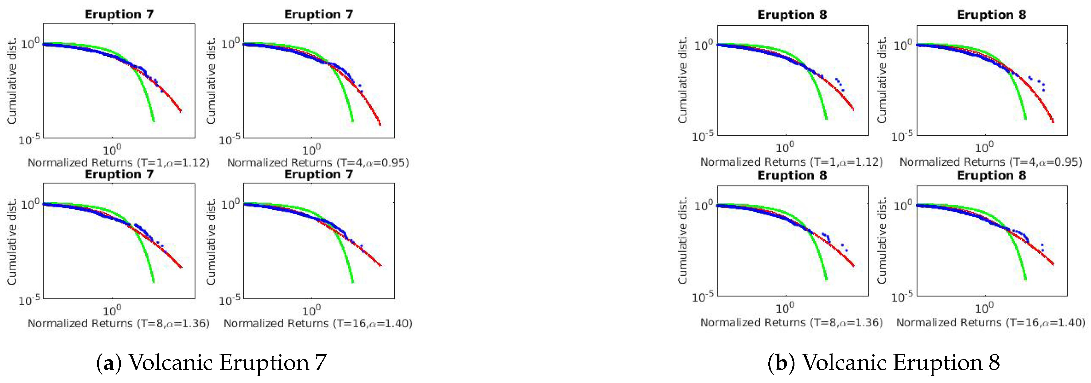
The Equation (10) represents the normalized Lévy model applied in this study. In the numerical simulations, we adjust the values of A, the arbitrary scale parameter l and the characteristic exponent α to best fit the cumulative function. Please refer to [2,23,24,25] for more details and Appendix B for figures.

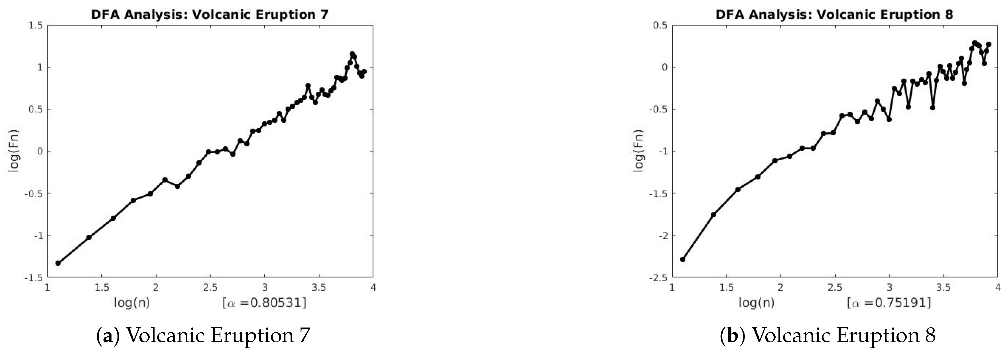
2.2. Detrended Fluctuation Analysis (DFA)

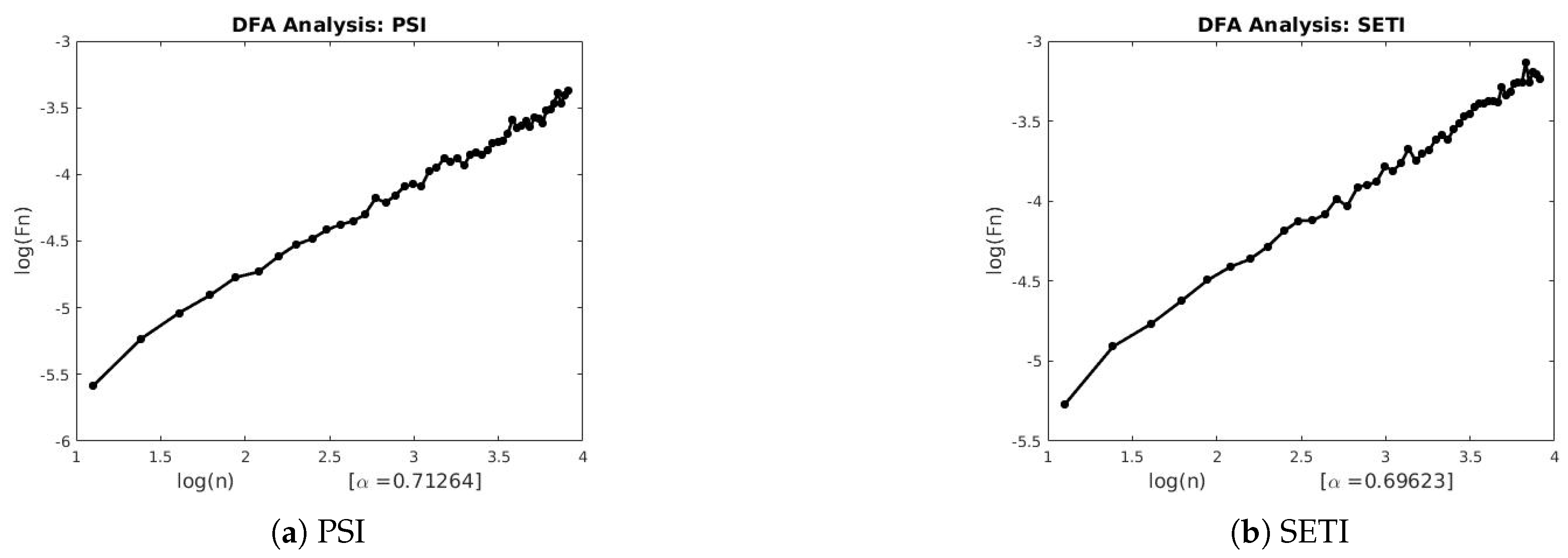
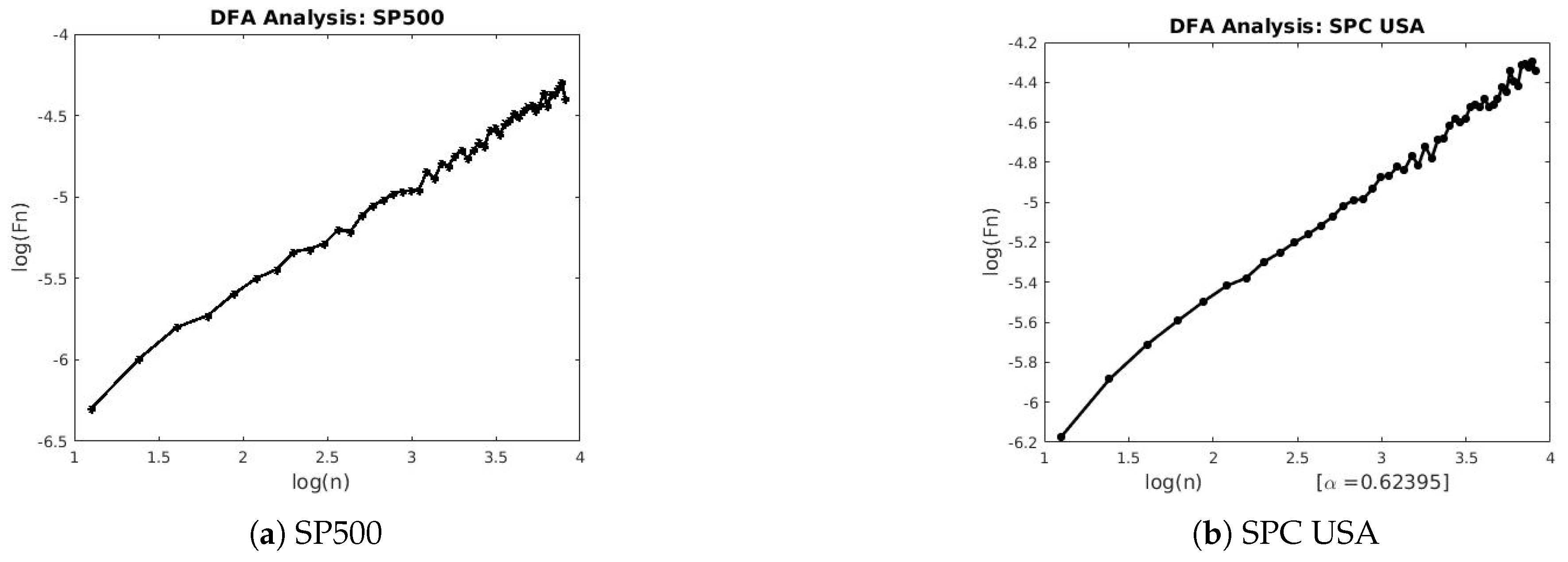
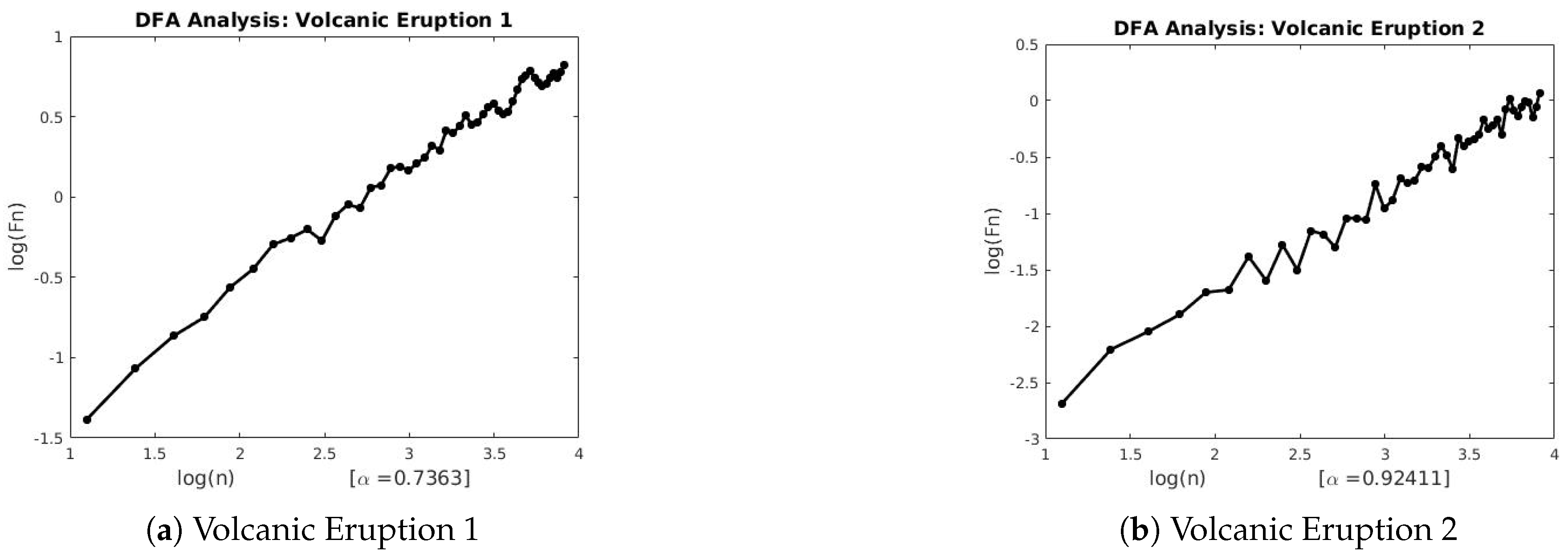
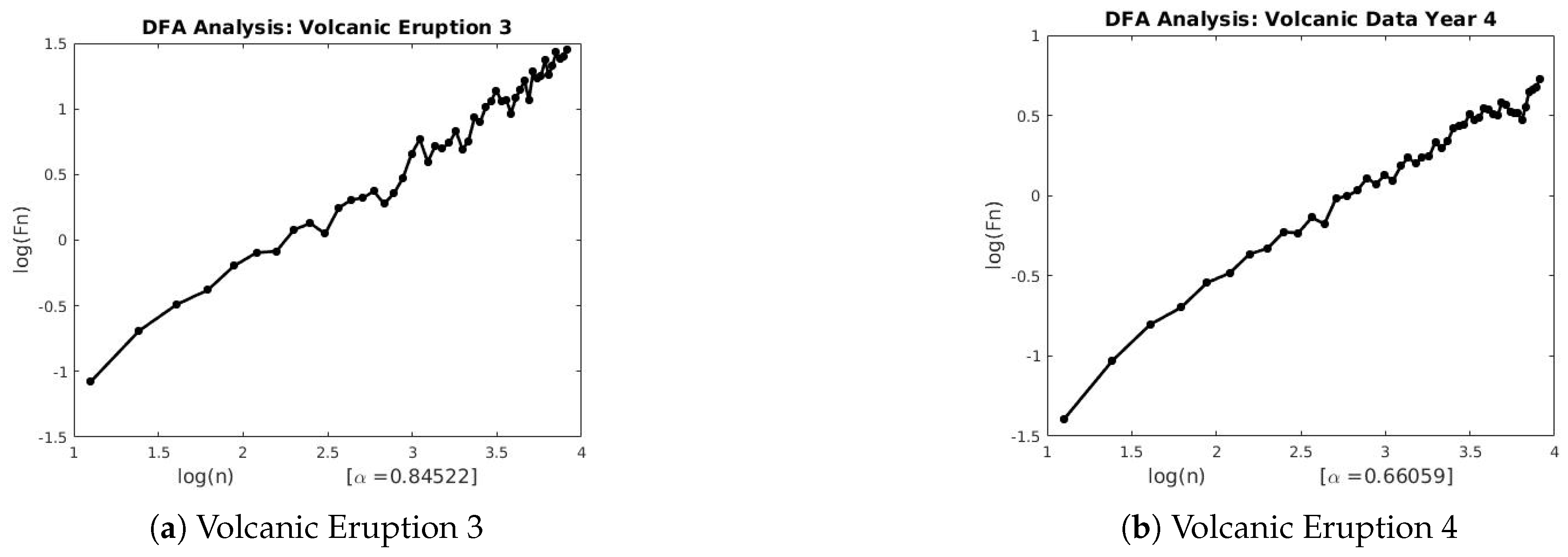
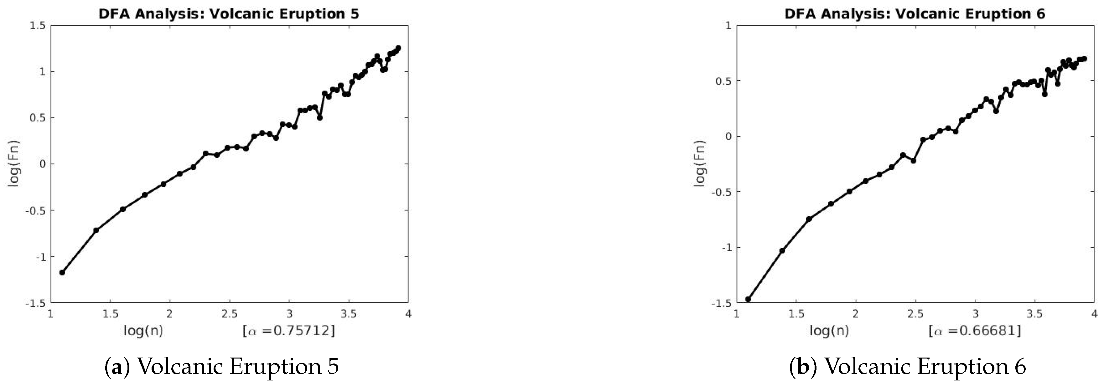
The DFA method is an important technique in revealing long range correlations in both stationary and non-stationary time series by estimating its scaling exponent. The numerical procedure to estimate the DFA exponent is presented below.

Let N be the length of time series $(y_1,y_2,y_3,\dots ,y_N)$. The logarithmic ratio of the time series is obtained and the length of the new time series $M\left(t\right)$ is $N-1$.

$$M\left(t\right)=log\left(\frac{y_{t+1}}{y_t}\right),t=1,2,\dots ,N-1$$

(11)

The absolute value of $M\left(t\right)$ is integrated:

$$y\left(t\right)=\sum _{i=1}^t\mid M\left(i\right)\mid$$

(12)

The integrated time series of length N is divided into m boxes of equal length n with no intersection between them. As the data is divided into equal length intervals, there may be some left over at the end. To take account of these leftover values, the same procedure is repeated but beginning from the end, obtaining $2N/n$ boxes.

A least square line is fitted to each box, representing the trend in each box, thus obtaining $y_n\left(t\right)$. Finally the Root Mean Square Fluctuation (RMSF) is calculated using the formula

$$F\left(n\right)=\sqrt{\frac{1}{2N}\sum _{t=1}^{2N}{\left[y\left(t\right)-y_n\left(t\right)\right]}^2}$$

(13)

This computation is repeated over all box sizes to characterize a relationship between the box size n and $F\left(n\right)$. A linear relationship between the $F\left(n\right)$ and n (i.e., box size) in a log-log plot reveals that the fluctuations can be characterized by a scaling exponent H, the slope of the line relating $logF\left(n\right)$ to $logn$. This generates the mathematical (power-law) relation:

$$F\left(n\right)\propto n^H$$

(14)

Next we discuss the Diffusion Entropy Analysis (DEA).

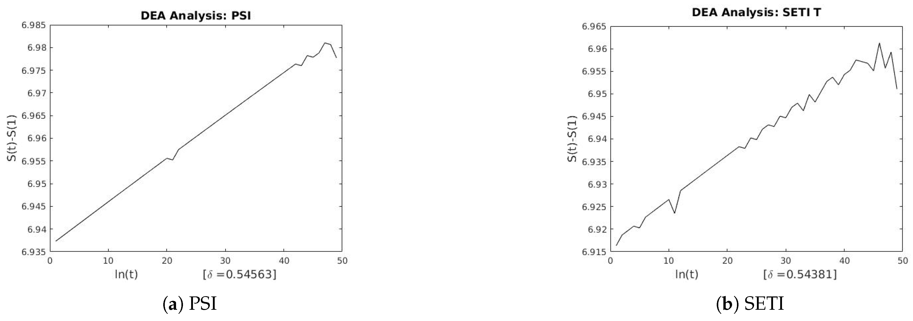
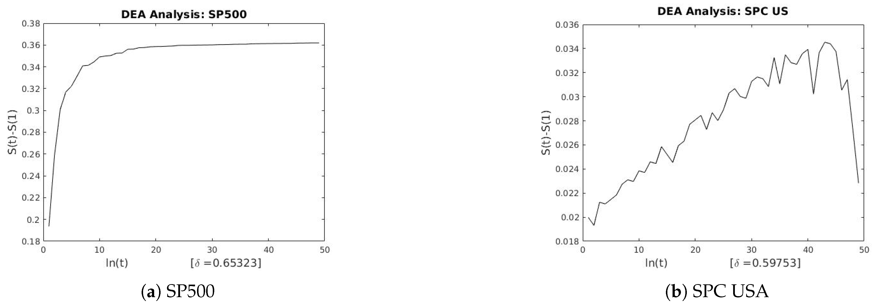
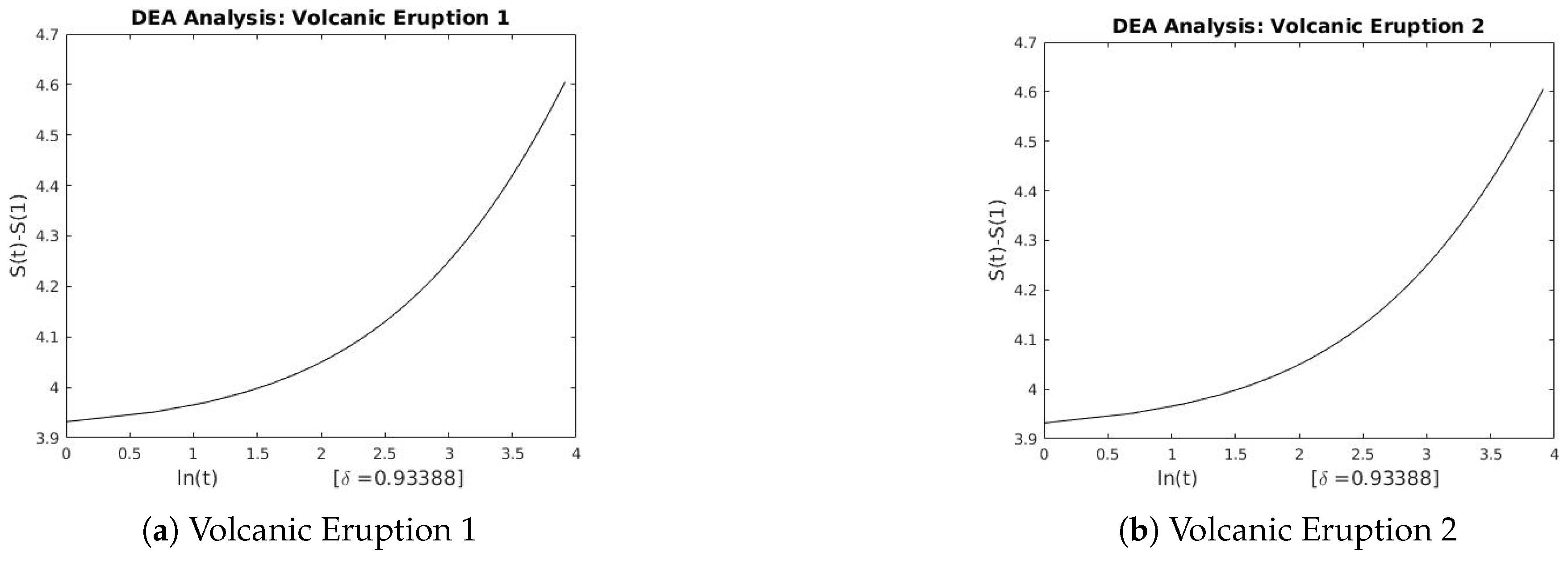
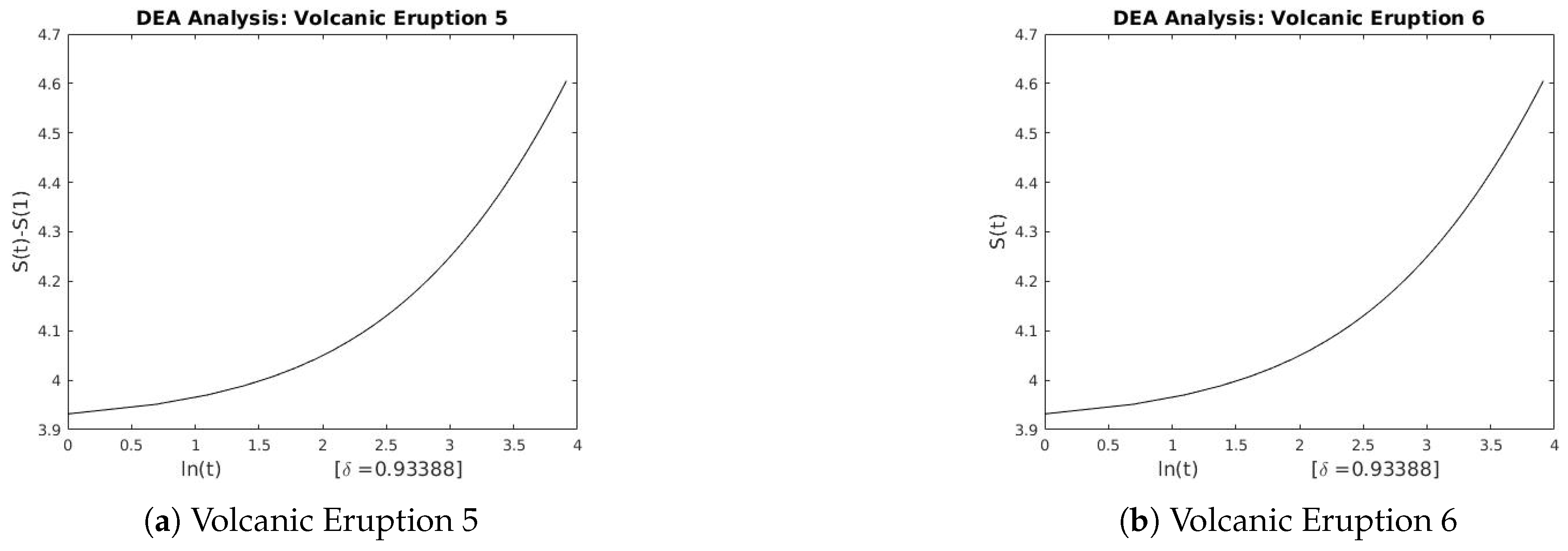
2.3. Diffusion Entropy Analysis (DEA)

The DEA can be used to analyze and detect the scaling properties of low and high frequency time series.

A function $\mathsf{\Phi }(r_1,r_2,\dots )$ is said to be invariant to scale changes if it fulfills the property:

$$\mathsf{\Phi }(r_1,r_2,\dots )={\gamma }^a\mathsf{\Phi }({\gamma }^b{r}_1,{\gamma }^c{r}_2,\dots ).$$

(15)

This equation shows that if we scale all coordinates r with an appropriate choice of exponents a, b, c, …, then we always recover the original function. In the case of a time series we can interpret the sequence of the numbers that form it as the generators of a diffusion process. Thus, we study the relevant probability distribution function $\rho (x,t)$ where x denotes the variable that collects the fluctuations of the diffusion process over time span t. If the time series is stationary, the scale property takes the shape

$$\rho (x,t)=\frac{1}{t^{\delta }}F\left(\frac{x}{t^{\delta }}\right),$$

(16)

where the δ is the scaling exponent.

To determine the scaling exponent of the DEA, first transform the series into a diffusion process and calculate its Shannon’s entropy.

Consider the equation

$$S\left(t\right)=-{\int }_{-\infty }^{\infty }\rho (x,t)ln\left[\rho (x,t)\right]dx$$

(17)

Suppose that $\rho (x,t)$ satisfies the scale condition (16), replacing it in the (17) we obtain:

$$S\left(t\right)=A+\delta ln\left(t\right)$$

(18)

Please see proof in Appendix A.

Equation (18) describes the fact that entropy grows linearly with $ln\left(t\right)$ and the slope of the linear function is the scaling exponent δ.

Let us now see how we generate the diffusion process for a sequence of M numbers:

$${ϵ}_i,i=1,\dots ,M$$

(19)

The purpose of the DEA algorithm is to establish the possible existence of scalability in an efficient way without altering the series with any form of detrending. We do the following:

• Select an integer l such that $1\le l\le M$.
• For each time, find $M-l+1$ sub-series of length l defined such that

  $${ϵ}_i^s\equiv {ϵ}_{i+s},i=1,\dots ,l$$

  (20)

  with $s=0,\dots ,M-l$.
• For each sub-series, construct a distribution diffusion path by the position

  $$x^{\left(s\right)}\left(l\right)=\sum _{i=1}^l{ϵ}_i^s=\sum _{i=1}^l{ϵ}_{i+s}$$

  (21)
• To calculate the Shannon entropy of the diffusion process, partition the $x-axis$ into size $\eta \left(l\right)$ cells and tell how many parts there are in each of them at a time l. Let us call this number $N_i\left(l\right)$.
• With $N\left(l\right)$, we determine the probability $p_i\left(l\right)$ that a particle is found in the i-th cell at time l.

  $$p_i\left(l\right)=\frac{N_i\left(l\right)}{M-l+1}$$

  (22)
• The entropy of the diffusion process at time l is given by

  $$S_d\left(l\right)=-\sum _i{p}_i\left(l\right)ln\left[p_i\left(l\right)\right]$$

  (23)

The sub-index d denotes that the entropy evaluation was generated from a discrete process. The reader should refer to [7,26,27,28] for more details.

2.4. Background of Data

In this subsection, we examine data from two different fields namely Financial Markets and Volcanic Eruptions and their stationary behavior.

2.4.1. Financial Market Data

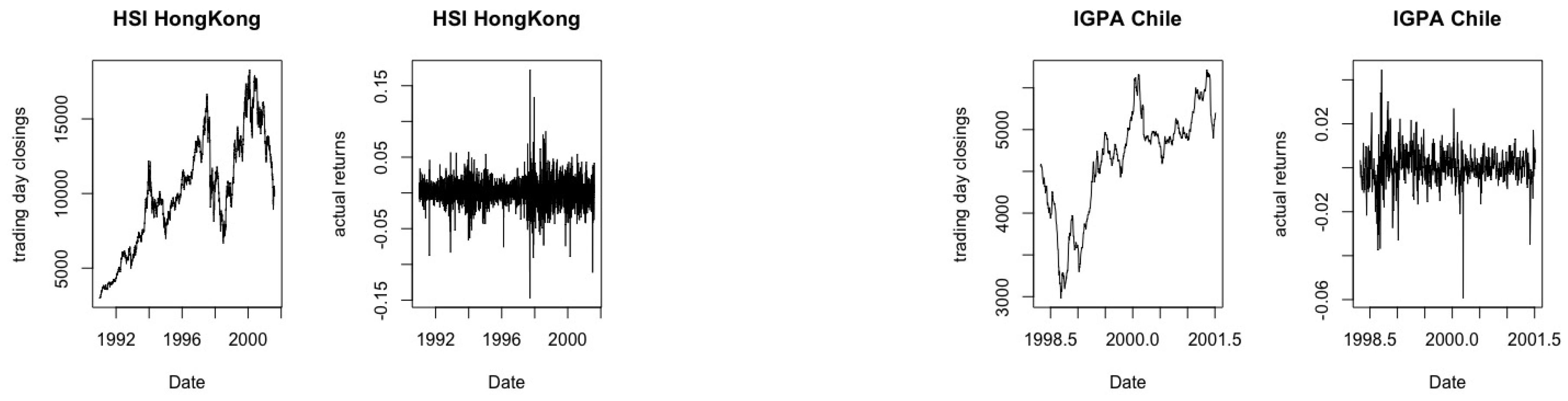
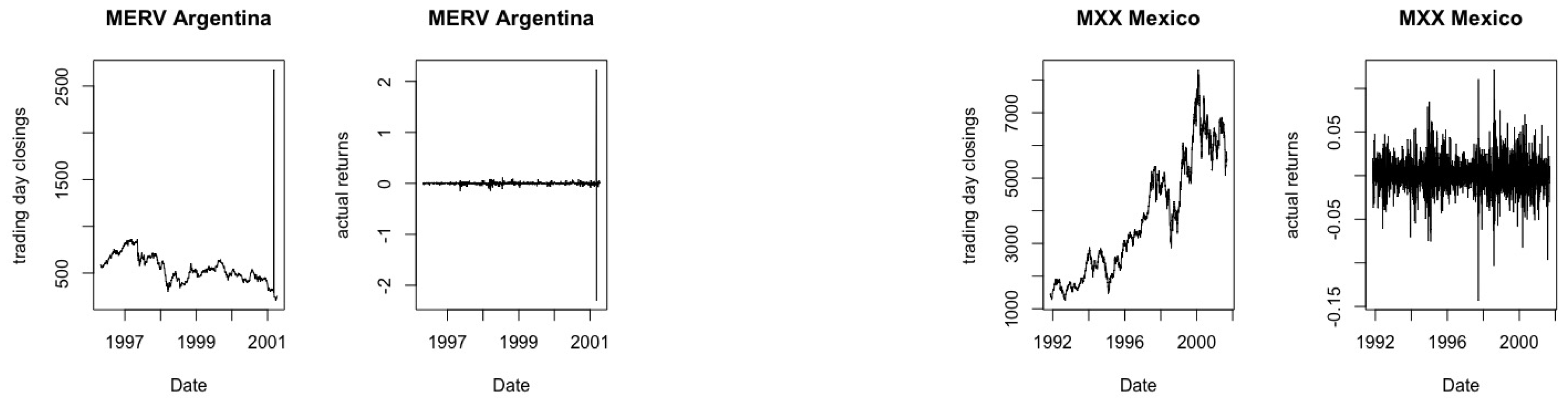
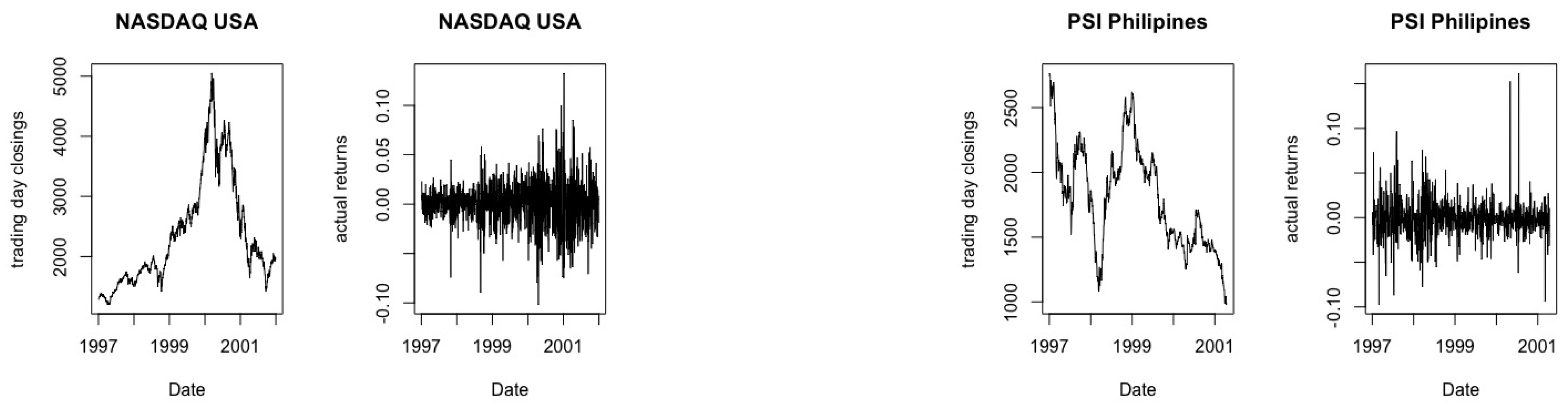
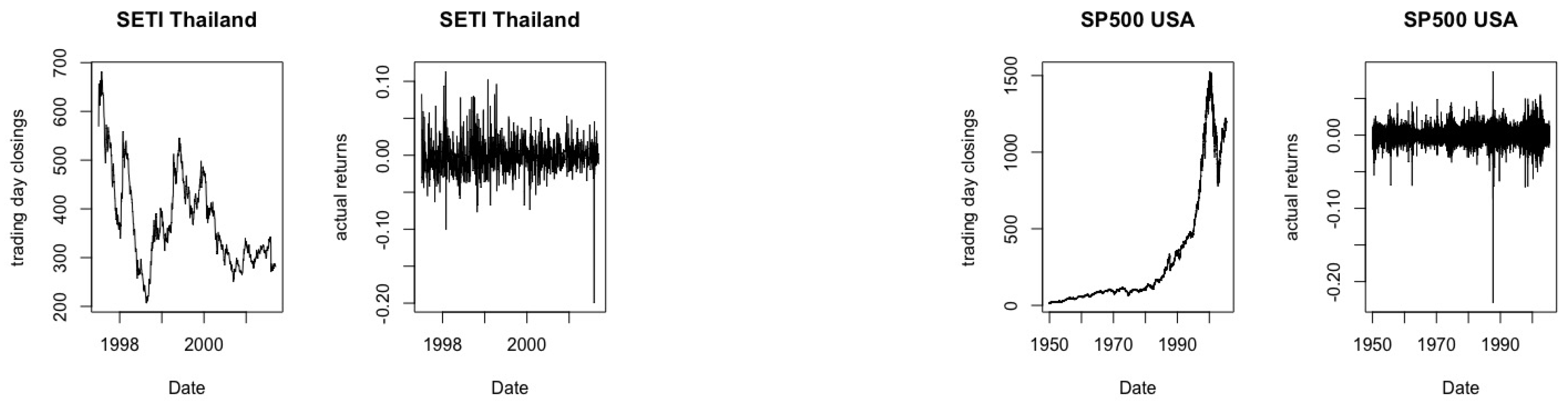
The financial market data used for the analysis in this paper was obtained from YAHOO FINANCE. All data points collected are daily close values. Below are the names of countries or cities where data was collected as well as the respective start and end dates of data collection: Brazil (BOVESPA), from 27 April 1993 to 24 June 2005; USA (SPC), from 2 January 1991 to 25 October 2001; Hong Kong (HSI), from 2 January 1991 to 25 October 2001; Chile (IGPA), from 28 April 1998 to 24 October 2001; Argentina (MERVAL), from 8 October 1996 to 22 October 2001; Mexico (MXX), from 8 November 1991 to 22 October 2001; USA (NASDAQ), from 22 January 1997 to 31 December 2001; Phillipines (PSI), from 2 July 1997 to 25 October 2001; Thailand (SETI), from 2 July 1997 to 25 October 2001 and USA (S&P500) from 2 January 1991 to 25 October 2001. This data was first used for big data analysis in [16] and recently used in [7]. The price evolution of the financial market time series are presented in Figure 2, Figure 3, Figure 4, Figure 5 and Figure 6.

2.4.2. Geophysical Time Series Data

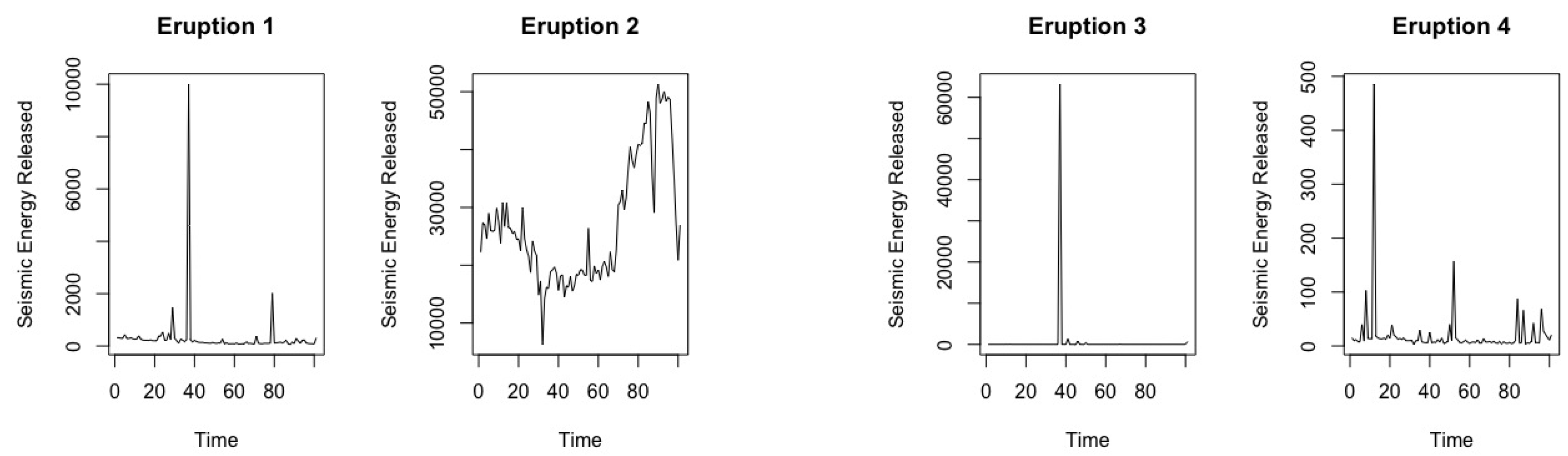
The Bezymianny Volcano Campaign Seismic Network (PIRE) collected the volcanic data at different eruption times at two different seismic stations, namely BEZB and BELO. Data used in this paper were requested for 10 days before and 5 days after the published time of the volcanic eruptions. Volcanic eruptions 1 and 2 were from BEZB and Volcanic eruptions 3–8 were from BELO. Please see [24] for more details on the geophysical time series used in this study. 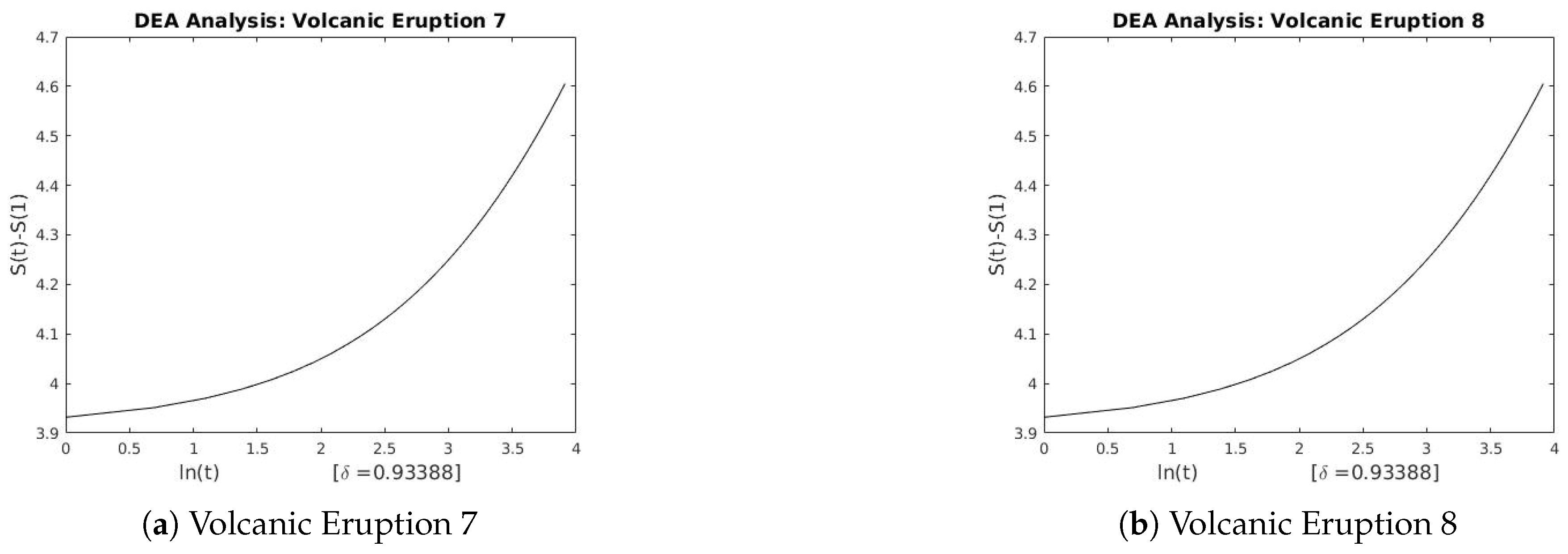The plots of the volcanic eruptions time series are presented in Figure 7 and Figure 8.

2.4.3. Stationarity Test of Data

We use the Augmented Dickey-Fuller (ADF) test to examine the stationarity of both the returns of the financial market data and volcanic data. The returns of the financial market data is calculated as:

$$marketreturns\left(r_t\right)=(X_t-X_{t-1})/X_{t-1}$$

where $X_t$ is the current market closing value and $X_{t-1}$ is the previous market closing value.

2.4.4. Augmented Dickey-Fuller (ADF)

The ADF statistic tests the null hypothesis that the time series has a unit root against the alternative that it is stationary (or has no unit root) with the assumption that the data exhibits an Auto-Regressive Moving Average (ARMA) structure.

• $H_0:\gamma =0$
• $H_a:\gamma <0$

The value of the ADF test statistic is computed as

$$AD{F}_{\tau }=\frac{\widehat{\gamma }}{SE\left(\widehat{\gamma }\right)}$$

As this test is asymmetrical, we are only concerned with negative values when it comes to the test statistic. If the calculated test statistic, $AD{F}_{\tau }$ is less (more negative) than the critical value, the null hypothesis is rejected and we conclude that no unit root is present and vice versa.

Based on the values obtained in

Table 1. ADF test results for returns of various financial markets.

Financial Market	Test Statistic	Lag Order	p-Value
BVSP	−16.571	12	0.01
SPC	−19.992	13	0.01
HSI	−18.937	13	0.01
IGPA	−10.87	9	0.01
MERV	−13.298	10	0.01
MXX	−12.496	13	0.01
Nasdaq	−7.4649	10	0.01
PSI	−10.207	10	0.01
SETI	−8.4743	10	0.01
SP500	−30.856	24	0.01

and

Table 2. ADF test results for different eruption times of Volcano at the two seismic stations.

Station	Eruption	Test Statistic	Lag Order	p-Value
BEZB	1	−3.155	7	0.10
	2	−1.946	7	0.60
BELO	3	−3.188	8	0.09
	4	−3.181	8	0.09
	5	−3.342	8	0.07
	6	−3.366	7	0.06
	7	−2.784	7	0.25
	8	−2.092	7	0.54

, at 95% level, the null hypothesis of a unit root is rejected because the $AD{F}_{\tau }$ test statistics of most data points is more negative than the critical value of −2.86 from the critical values for Dickey-Fuller t-distribution [29]. We further confirm this conclusion using the p-values at a significant level of $\alpha =5\%$. All p-values of both the returns of the financial market data and the volcanic eruption data are less than the significance level (0.05).

We reject the null hypothesis that the time series has a unit root and conclude that both the returns of financial market data and the data from different eruption times of the volcano are stationary.

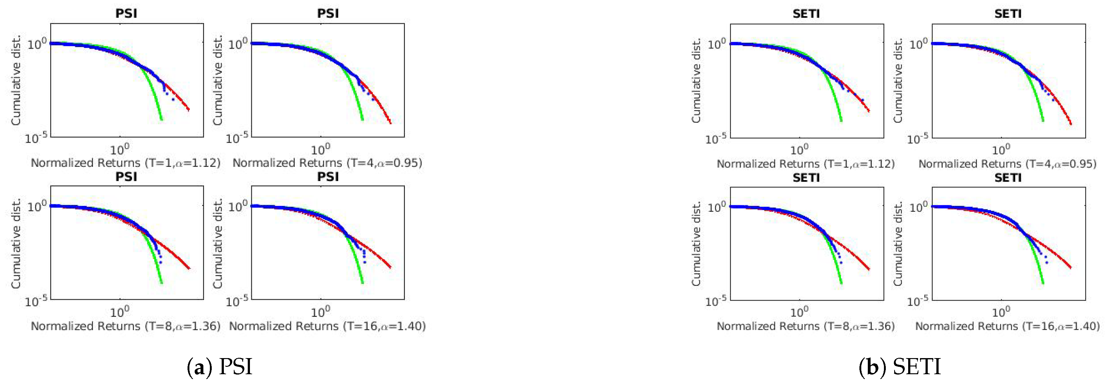
3. Results

In this section, we present numerical results obtained from applying all 3 models to the data. From our numerical results we propose a mathematical relationship between the self-similar models and the Lévy model. We also present an analytical proof of the numerically derived relationship.

3.1. Numerical Results

Below are tables for both the financial markets data and volcanic eruption data. There are six (6) columns in each table where the first column indicates the particular financial market or volcanic eruption numbers, the second - fourth columns show the scaling exponents of the DFA and the DEA as well as the best Lévy parameter α characterizing the data. The last three columns are basically products of the respective scaling exponents of the self-similar models $H,\delta$ and the Lévy parameter α characterizing the data.

Remarks on the Tables of Numerical Results

Empirical evidence presented in

Table 3. Scaling exponents of various financial markets.

Markets	DFA (H)	DEA (δ)	Lévy (α)	H.α	δ.α
BVSP	0.72	0.57	1.34	0.96	0.76
SPC	0.62	0.60	1.40	0.87	0.84
HSI	0.70	0.60	1.40	0.98	0.84
IGPA	0.65	0.53	1.40	0.91	0.74
MERV	0.62	0.56	1.40	0.87	0.78
MXX	0.66	0.59	1.34	0.90	0.79
Nasdaq	0.72	0.56	1.12	0.96	0.66
PSI	0.71	0.55	1.40	0.99	0.77
SETI	0.70	0.54	1.34	0.94	0.72
SP500	0.66	0.65	1.40	0.92	0.91

and

Table 4. Scaling exponents of Volcanic Data from the two seismic stations.

Seismic Station	Eruption Number	DFA (α)	DEA (δ)	Lévy (α)	H.α	δ.α
BEZB	1	0.74	0.68	1.12	0.83	0.76
	2	0.92	0.68	1.34	1.23	0.91
BELO	3	0.85	0.68	1.12	0.95	0.76
	4	0.66	0.68	1.40	0.92	0.95
	5	0.76	0.68	1.12	0.85	0.76
	6	0.67	0.68	1.34	0.90	0.91
	7	0.81	0.68	1.40	1.13	0.95
	8	0.75	0.68	1.34	1.01	0.91

show that the product of respective scaling exponents of the DFA and Lévy as well as DEA and Lévy approximately equal 1. This suggests that there exist an inverse relationship between the DEA parameter δ and the Lévy parameter α, i.e.,:

$$\delta \approx \frac{1}{\alpha }$$

(24)

Also, an inverse relationship exists between the DFA parameter H and the resulting Lévy parameter α, i.e.,:

$$\mathit{H}\approx \frac{1}{\alpha }$$

(25)

3.2. Analytical Relations

In this section, we prove analytically the numerical relations obtained from the previous subsection.

Property 1

(Stable distributions). Given a random variable X, if we denote with $Law\left(X\right)$ its probability density function (for example, for a Gaussian random variable, we write $Law\left(X\right)=N(\mu ,{\sigma }^2)$) then we will say that the random variable X is stable, or that it has a stable distribution if for any $n\ge 2$ there exists a positive number $C_n$ and a number $D_n$ so that:

$$Law(X_1+X_2+\dots +X_n)=Law(C_{n}X+D_n)$$

(26)

where $X_1,X_2,\dots ,X_n$ are independent random copies of X, this means that $Law\left(X_i\right)=Law\left(X\right)$ for $i=1,2,\dots ,n$. If $D_n=0$, then X is said to be a strictly stable variable. It can be shown (see Samorodnitsky and Taqqu (1994)) that

$$C_n=n^{1/\alpha }$$

(27)

for some parameter $0<\alpha \le 2$.

Equation (27) can be rewritten as

$$log{C}_n=\frac{1}{\alpha }logn$$

(28)

3.2.1. Detrended Fluctuation Analysis (DFA)

From (14), we obtain a mathematical relation that reveals a linear relationship between the root mean square fluctuation $F\left(n\right)$ and the box size n in a log-log plot. i.e.,

$$logF\left(n\right)=logK+Hlog\left(n\right)$$

(29)

where K is a positive constant of proportionality.

$$logF\left(n\right)-logK=Hlog\left(n\right)$$

(30)

Subtracting (30) and (28) gives the relation:

$$H=1/\alpha$$

since

$$\underset{n\to \infty }{lim}\mid \frac{logF\left(n\right)-logK-log{C}_n}{logn}\mid \to 0$$

(31)

3.2.2. Diffusion Entropy Analysis (DEA)

From the probability density function (pdf) in (16), one can calculate the Shannon entropy [2,23],

$$S\left(t\right)=-{\int }_{-\infty }^{\infty }\rho (x,t)ln\left[\rho (x,t)\right]dx$$

(32)

Suppose the pdf $\rho (x,t)$ satisfies (16), then after a few simple steps (see appendix for proof) [23], we obtain the linear-log relation

$$S\left(t\right)=A+\delta ln\left(t\right)$$

(33)

where Equation (33) becomes

$$S\left(t\right)-S\left(1\right)=\delta ln\left(t\right)$$

(34)

From property 1, for some positive number $C_n$, subtracting (34) and (28) gives

$$|S\left(t\right)-S\left(1\right)-ln\left(C_n\right)|=0,wheret\ge 2$$

(35)

such that

$$\delta =\frac{1}{\alpha }$$

4. Discussion

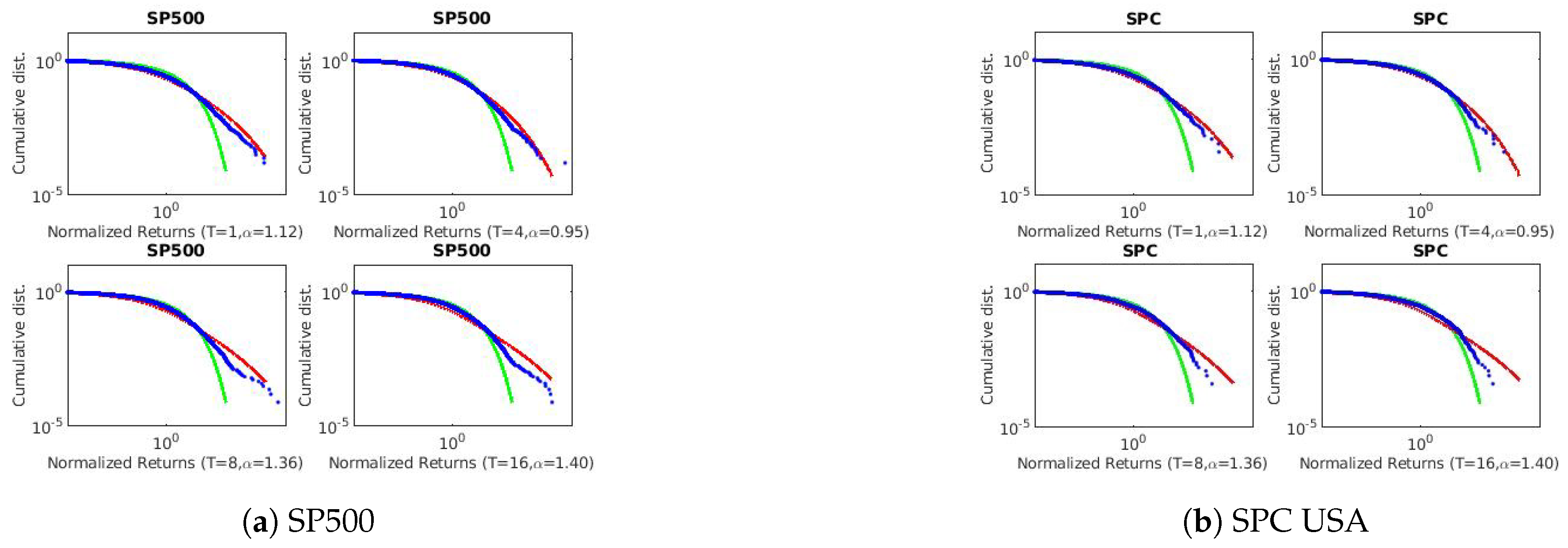
The three techniques described in Section 2 were used to estimate the scaling exponents of the financial and geophysical time series. Table 3 and Table 4 summarizes the results of each technique applied to the real-world data. Figure A1, Figure A2, Figure A3, Figure A4, Figure A5, Figure A6, Figure A7, Figure A8, Figure A9, Figure A10, Figure A11, Figure A12, Figure A13, Figure A14, Figure A15, Figure A16, Figure A17 and Figure A18 in the appendix provide a graphical summary of results from techniques used in this paper. The results confirm an inverse relationship between the self-similar parameters $(H,and\delta )$ and the Lévy flight parameter. We also observe the existence of long-range persistence in the financial and geophysical time series which confirms seasonal or irregular occurrence of real-world events such as stock market crushes and volcanoes of the past. They are helpful in the forecasting of such events using past and recent information.

Having proved the existence of an inverse relationship between the Lévy parameter and the scaling parameters of the DFA and DEA, in the event that the scaling exponent of either of the parameter estimators is not known or expensive to estimate, we are able to approximate it using the relationship generated in this study. This is because data keeps getting bigger, making the measurements and collections of big data more expensive and time-consuming.

In future work, we seek to investigate whether some of the scaling methods significantly outperform others using real-world time series with removed components such as trends, seasonality and irregularities (noise). This experiment is essential to undertake partly due to complications in measurement and collection of real-world data especially in fast-paced industries such as the financial sector.

5. Conclusions

In this study, we compare and quantify the scaling parameters depicting long-range persistence behavior of a set of financial and geophysical time series using the DFA and DEA techniques. We also characterize the respective time series with Lévy process (with stable distributions) to obtain the best Lévy flight parameter. Both the financial and the geophysical time series exhibit long-range correlations since $0.5<H$, $\delta <1$. Empirical evidence from results suggest an inverse relationship between the DFA parameter H and the resulting Lévy parameter α. Similarly, an inverse relationship exists between the DEA parameter δ and the Lévy parameter α.

Finally, we present proofs to verify these mathematical relationships. However, one has to note that the choice of the α parameter for the Lévy processes means they are stochastic. They are influenced by the respective time variables, $T=1,4,8,16$. The appropriate Lévy parameter is selected at appropriate time periods. Another limitation of this study is that, we adjust the values of A, the arbitrary scale parameter l and the characteristic exponent α of the Lévy flight model in the numerical simulations to get the best fit of the cumulative distribution function of the Lévy process. It is also worth noting that because we standardized the Lévy model we should only expect an approximate inverse relationship between the self-similar parameters $(H,\delta )$ and the Lévy parameter $\left(\alpha \right)$.

References

1. Mandelbrot, B.B. The Fractal Geometry of Nature; Times Books: New York, NY, USA, 1982; p. 44. [Google Scholar]
2. Barany, E.; Beccar Varela, M.P.; Florescu, I.; Sengupta, I. Detecting market crashes by analyzing long-memory effects using high-frequency data. Quant. Financ. 2012, 12, 623–634. [Google Scholar] [CrossRef]
3. Peng, C.K.; Buldyrev, S.V.; Havlin, S.; Simons, M.; Stanley, H.E.; Goldberger, A.L. Mosaic organization of DNA nucleotides. Phys. Rev. E 1994, 49, 1685–1689. [Google Scholar] [CrossRef] [PubMed] [Green Version]
4. Shlesinger, M.F.; West, B.J.; Klafter, J. Lévy dynamics of enhanced diffusion: Application to turbulence. Phys. Rev. Lett. 1987, 58, 11–16. [Google Scholar] [CrossRef] [PubMed]
5. Ben-Avraham, D.; Havlin, S. Diffusion and Reactions in Fractals and Disordered Systems; Cambridge University Press: Cambridge, UK, 2000. [Google Scholar]
6. Scafetta, N. An Entropic Approach to the Analysis of Time Series; University of North Texas: Denton, TX, USA, 2003; p. 5906. [Google Scholar]
7. Mariani, M.C.; Asante, P.K.; Bhuiyan, M.A.M.; Beccar-Varela, M.P.; Jaroszewicz, S.; Tweneboah, O.K. Long-Range Correlations and Characterization of Financial and Volcanic Time Series. Mathematics 2020, 8, 441. [Google Scholar] [CrossRef] [Green Version]
8. Buldyrev, S.V.; Goldberger, A.L.; Havlin, S.; Mantegna, R.N.; Matsa, M.E.; Peng, C.K.; Simons, M.; Stanley, H.E. Long-Range Correlation-Properties of Coding And Noncoding DNA-Sequences—Genbank Analysis. Phys. Rev. E 1995, 51, 508–5091. [Google Scholar] [CrossRef] [PubMed]
9. Bunde, A.; Havlin, S. Fractals and Disordered Systems; Springer: Berlin/Heidelberg, Germany, 1996. [Google Scholar]
10. Kantelhardt, J.W.; Koscielny-Bunde, E.; Rego, H.H.A.; Havlin, S.; Bunde, A. Detecting Long-range Correlations with Detrended Fluctuation Analysis. Phys. A 2001, 295, 441–454. [Google Scholar] [CrossRef] [Green Version]
11. Hardstone, R.; Poil, S.S.; Schiavone, G.; Jansen, R.; Nikulin, V.V.; Mansvelder, H.D.; Linkenkaer-Hansen, K. Detrended Fluctuation Analysis: A Scale-Free View on Neuronal Oscillations. Front. Physiol. 2012, 3, 450. [Google Scholar] [CrossRef] [PubMed] [Green Version]
12. Little, M.; McSharry, P.; Moroz, I.; Roberts, S. Nonlinear, Biophysically-Informed Speech Pathology Detection. IEEE Int. Conf. Acoust. Speed Signal Process. Proc. 2006, 2, 1080–1083. [Google Scholar]
13. Bunde, A. Correlated and uncorrelated regions in heart-rate fluctuations during sleep. Phys. Rev. E 2000, 85, 373–3739. [Google Scholar] [CrossRef] [PubMed] [Green Version]
14. Mantegna, R.N.; Stanley, H.E. Stochastic process with ultra-slow convergence to a Gaussian: the truncated Lévy flight. Phys. Rev. Lett. 1994, 73, 2946–2949. [Google Scholar] [CrossRef] [PubMed]
15. Koponen, I. Analytic approach to the problem of convergence of truncated Lévy flights towards the Gaussian stochastic process. Phys. Rev. E 1995, 52, 1197–1199. [Google Scholar] [CrossRef] [PubMed]
16. Mariani, M.C.; Liu, Y. Normalized truncated Lévy walks applied to the study of financial indices. Phys. A 2007, 377, 590–598. [Google Scholar] [CrossRef]
17. Kleinberg, J.M. Navigation in a small world. Nature 2000, 406, 845. [Google Scholar] [CrossRef] [PubMed]
18. Li, G.; Reis, S.D.S.; Moreira, A.A.; Havlin, S.; Stanley, H.E.; Andrade, J.S., Jr. Towards Design Principles for Optimal Transport Networks. Phys. Rev. Lett. 2010, 104, 018701. [Google Scholar] [CrossRef]
19. Viswanathan, G.M.; Buldyrev, S.V.; Havlin, S.; da Luz, M.G.E.; Raposo, E.P.; Stanley, H.E. Optimizing the success of random searches. Nature 1999, 401, 910–914. [Google Scholar] [CrossRef] [PubMed]
20. Reynolds, G. Navigating Our World Like Birds and some authors have claimed that the motion of bees. The New York Times, 1 January 2014. [Google Scholar]
21. Sims, D.W.; Reynolds, A.M.; Humphries, N.E.; Southall, E.J.; Wearmouth, V.J.; Metcalfe, B.; Twitchett, R.J. Hierarchical random walks in trace fossils and the origin of optimal search behavior. Proc. Natl. Acad. Sci. USA 2014, 111, 1107–1108. [Google Scholar] [CrossRef] [PubMed] [Green Version]
22. Khintchine, A.Y.; Lévy, P. Sur les lois stables. CR Acad. Sci. Paris 1936, 202, 374–376. [Google Scholar]
23. Mariani, M.C.; Florescu, I.; Beccar Varela, M.P.; Ncheuguim, E. Long correlations and Lévy models applied to the study of memory effects in high frequency (tick) data. Phys. A Stat. Mech. Its Appl. 2009, 388, 1659–1664. [Google Scholar] [CrossRef]
24. Beccar-Varela, M.P.; Gonzalez-Huizar, H.; Mariani, M.C.; Tweneboah, O.K. Lévy Flights and Wavelets Analysis of Volcano-Seismic Data. Pure Appl. Geophys. 2020, 177, 723–736. [Google Scholar] [CrossRef]
25. Beccar-Varela, M.; Gonzalez-Huizar, H.; Mariani, M.C.; Serpa, L.F.; Tweneboah, O.K. Chile2015: Lévy Flight and Long-Range Correlation Analysis of Earthquake Magnitudes in Chile. In The Chile-2015 (Illapel) Earthquake and Tsunami; Birkhäuser: Cham, Switzerland, 2017; pp. 113–122. [Google Scholar]
26. Scafetta, N.; Grigolini, P. Scaling detection in time series: Diffusion entropy analysis. Phys. Rev. E 2002, 66, 036130. [Google Scholar] [CrossRef] [PubMed] [Green Version]
27. Clausius, R. Available online: http://www.ueltschi.org/teaching/chapShannon.pdf (accessed on 15 October 2019).
28. Clausius, R. Available online: http://galileo.phys.virginia.edu/classes/152.mf1i.spring02/Entropy.pdf (accessed on 10 October 2019).
29. Fuller, W.A. Introduction to Statistical Time Series; John Wiley and Sons: New York, NY, USA, 1976. [Google Scholar]
Figure 1. Figure of Koch snowflake curve depicting self-similarity.
Mathematics 08 01046 g001
Figure 2. Plots of trading days closings and actual returns of BVSP and SPC.
Mathematics 08 01046 g002
Figure 3. Plots of trading days closings and actual returns of HSI and IGPA.
Mathematics 08 01046 g003
Figure 4. Plots of trading days closings and actual returns of MERV and MXX.
Mathematics 08 01046 g004
Figure 5. Plots of trading days closings and actual returns of Nasdaq and PSI.
Mathematics 08 01046 g005
Figure 6. Plots of trading days closings and actual returns of SETI and SP500.
Mathematics 08 01046 g006
Figure 7. Plots of volcanic eruption numbers 1, 2, 3 and 4.
Mathematics 08 01046 g007
Figure 8. Plots of volcanic eruption numbers 5, 6, 7 and 8.
Mathematics 08 01046 g008