Semi-Implicit Multistep Extrapolation ODE Solvers

Abstract

Multistep methods for the numerical solution of ordinary differential equations are an important class of applied mathematical techniques. This paper is motivated by recently reported advances in semi-implicit numerical integration methods, multistep and extrapolation solvers. Here we propose a novel type of multistep extrapolation method for solving ODEs based on the semi-implicit basic method of order 2. Considering several chaotic systems and van der Pol nonlinear oscillator as examples, we implemented a performance analysis of the proposed technique in comparison with well-known multistep methods: Adams–Bashforth, Adams–Moulton and the backward differentiation formula. We explicitly show that the multistep semi-implicit methods can outperform the classical linear multistep methods, providing more precision in the solutions for nonlinear differential equations. The analysis of stability regions reveals that the proposed methods are more stable than explicit linear multistep methods. The possible applications of the developed ODE solver are the long-term simulations of chaotic systems and processes, solving moderately stiff differential equations and advanced modeling systems.

1. Introduction

In recent years, tools for computer simulation have become increasingly important in various fields of science. Computational experiments allow one to obtain new knowledge about the properties and dynamics of the object under investigation without the significant economic and time costs and risks that attend a full-scale experiment. To study the continuous dynamical systems described by ordinary differential equations (ODE), numerical integration methods are traditionally used. While the scale and complexity of the systems under investigation increase, one needs more sophisticated and efficient integration techniques [1]. Therefore, the advanced numerical methods used to simulate dynamical systems should possess great stability, precision and low computational costs. In engineering applications, especially while solving high-dimensional initial value problems (IVP), multistep integration is widespread [2].

Being compared to their single-step counterparts, multistep methods employ one call to the right-hand-side function per each integration step. To obtain the numerical solution with the desired accuracy, such algorithms reuse values calculated at previous steps. Therefore, multistep algorithms significantly exceed single-step integration in computational speed. However, the well-known problem of such integration is a decrease in numerical stability with an increase in the accuracy order of the chosen scheme. This property restricts the application of high-order multistep methods for solving stiff ODE systems excluding implicit methods, such as backward differentiation formulas (BDF) [3]. However, the application of implicit methods involves computationally expensive approximation of the numerical solution at the next point using Newton’s method or some other iterative technique. This fact eliminates one of the main advantages of multistep algorithms—their computational simplicity and high efficiency.

Several approaches that circumvent the so-called Dahlquist order barrier, including the second derivative multistep method [4], hybrid linear multistep methods [5,6,7], and extended backward differentiation formulas [8], were recently proposed. Being applied to the stiff ODEs, such methods have shown high numerical efficiency.

Recent studies also revealed the possibility to construct efficient implicit–explicit linear multistep methods for stiff problems [5,6,9]. One of the prospective techniques combining the advantages of implicit and explicit integration for the numerical solution of differential equations is semi-implicit integration. High-performance compositional [10] ODE solvers based on semi-implicit single-step calculations have been proposed. Efficient techniques for non-Hamiltonian systems [11] simulation were developed based on Aitken–Neville extrapolation and the semi-implicit symmetric basic method [12]. It has been shown that, compared with other integration algorithms, semi-implicit methods demonstrate good stability and low computational costs, which allows outperforming both explicit and implicit techniques [13]. Thus, semi-implicit integration no longer remains a specialized tool for Hamiltonian systems and can be efficiently applied to the general class of initial value problems (IVP).

One of the most efficient single-step numerical integration techniques is extrapolation solvers [4]. The well-known ODEx solver, based on the Gragg–Bulirsch–Stoer method, is one of the most efficient explicit integration methods [14]. Being implemented with adaptive stepsize it can be even more numerically efficient than embedded Runge-Kutta methods [15]. However, although the first studies of extrapolation multistep schemes have been known since the 1970s [12], there are no multistep extrapolation solvers presented in the modern simulation software. Thus, it is of interest to develop semi-implicit multistep methods based on numerical extrapolation techniques. In this paper, we suggest closing this gap by introducing a novel multistep ODE solver combining the advantages of the extrapolation technique and the semi-implicit symmetric basic method.

The rest of the paper is organized as follows. In Section 2, a novel type of multistep integration methods is described and tables of coefficients are given for solvers of order 3–6 in “full” and “short” form. Section 3 represents the set of computational experiments. We introduce several nonlinear test systems and estimate the computational efficiency of the compared methods through performance plots. In Section 4, we investigate the stability and convergence of ESIMM methods. Finally, in Section 5, some conclusions and discussion are given.

2. Materials and Methods

Consider a basic symmetric integration method for solving IVP of order p. A sequence of local error terms after stepping from the point x_n to x_n+1 with a stepsize h reads

$$x(t_{n+1})=x_{n+1}+h^{p+1}{e}_{p+1}+h^{p+2}{e}_{p+2}+\dots$$

(1)

A sequence of local error terms after stepping from the previous point x_n−1 to x_n+1 with a stepsize 2h reads

$$x(t_{n+1})=x_{n+1}+2^{p+1}{h}^{p+1}{e}_{p+1}+2^{p+2}{h}^{p+2}{e}_{p+2}+\dots$$

(2)

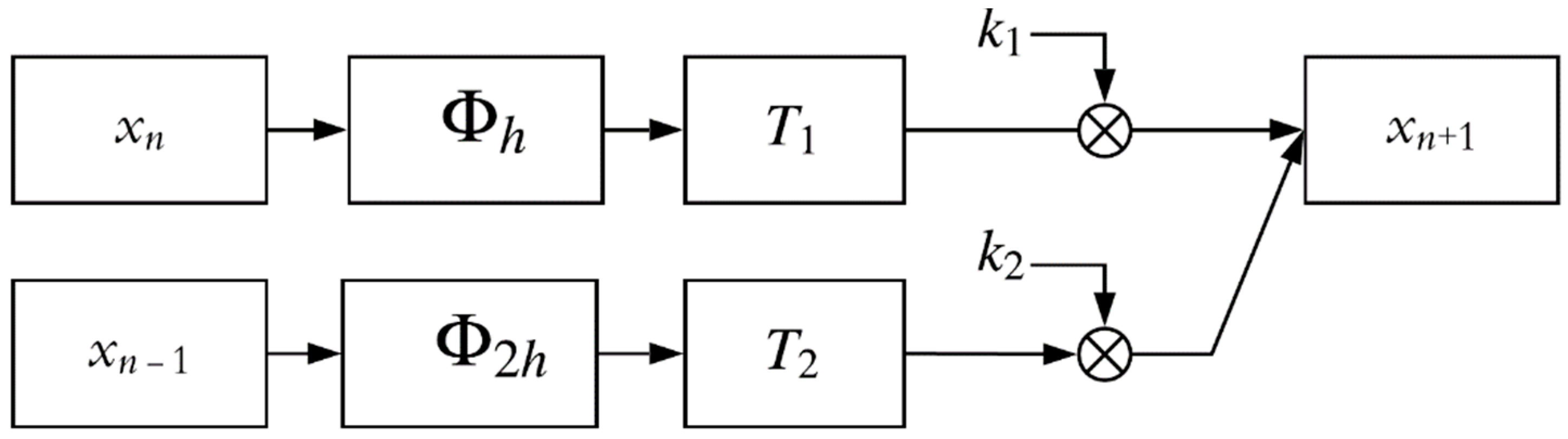
Following the idea of extrapolation methods [4,12], let us combine the solution at the point n + 1 with the stepsize h (denote it as T₁) and the solution at the same point with the stepsize 2h (denote it as T₂) as follows:

$$x_{n+1}=k_1{T}_1+k_2{T}_2$$

(3)

The dataflow representation of this combination is depicted in Figure 1. Keeping in mind Aitken-Neville interpolation rule, let us select the coefficients k₁ and k₂ so as to satisfy the following conditions:

$$\{\begin{array}{l}{k}_1+k_2=1\\ k_1+2^{p+1}{k}_2=0\end{array}$$

(4)

The system of Equation (4) can be analytically solved as

$$\{\begin{array}{l}{k}_1=\frac{2^{p+1}}{2^{p+1}-1}\\ k_2=\frac{-1}{2^{p+1}-1}\end{array}$$

For example, for the method of order 3 with p = 2 we have:

$$k_1=\frac{8}{7},k_2=\frac{-1}{7}$$

This allows eliminating the term by the error e_p+1 and increasing the order by one.

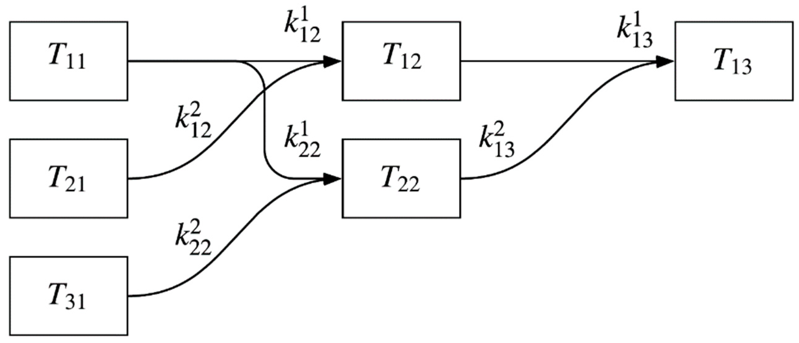
Let us organize the computational process in a cascade manner as shown in Figure 2. The main term T_ij represents a component in the extrapolation table on i-th stage on the j-th line. Indices by coefficients $k_{ij}^m$ are the following: m denotes whether it is the coefficient by the first or the second term, with the sum giving the term T_ij.

A general form for increasing an order can be obtained if we consider how the operation (3) affects the error terms in (1) and (2). Introducing the matrix formalism, for the coefficients on the first stage one can obtain

$$k_{12}=\left(\begin{array}{l}{k}_{12}^1\\ k_{12}^2\end{array}\right);\left(\begin{array}{cc}1& 1\\ 1& 2^{p+1}\end{array}\right)\left(\begin{array}{l}{k}_{12}^1\\ k_{12}^2\end{array}\right)=\left(\begin{array}{c}1\\ 0\end{array}\right)$$

(5)

After the first stage of extrapolation, equations for two approximations of $x\left(t_{n+1}\right)$ denoted as $T_{12}$ and $T_{22}$, which are then multiplied by $k_{13}^1$ and $k_{13}^2$ respectively, are as follows:

$$T_{12}=x_{n+1}+\left(k_{12}^1{h}^{p+2}+k_{12}^2{\left(2h\right)}^{p+2}\right)e_{p+2}+\dots$$

$$T_{22}=x_{n+1}+\left(k_{22}^1{h}^{p+2}+k_{22}^2{\left(3h\right)}^{p+2}\right)e_{p+2}+\dots$$

Let us rewrite them using a vector form:

$$T_{12}=x_{n+1}+(\begin{array}{cc}{k}_{12}^1& k_{12}^2)\left(\begin{array}{c}1\\ 2^{p+2}\end{array}\right)\end{array}{h}^{p+2}{e}_{p+2}+\dots$$

$$T_{22}=x_{n+1}+(\begin{array}{cc}{k}_{22}^1& k_{22}^2)\left(\begin{array}{c}1\\ 3^{p+2}\end{array}\right)\end{array}{h}^{p+2}{e}_{p+2}+\dots$$

Similar to the Equation (5), the final equation for $k_{13}$ reads:

$$k_{13}=\left(\begin{array}{c}{k}_{13}^1\\ k_{13}^2\end{array}\right);\left(\begin{array}{cc}1& 1\\ k_{12}^T\left(\begin{array}{c}1\\ 2^{p+2}\end{array}\right)& k_{13}^T\left(\begin{array}{c}1\\ 3^{p+2}\end{array}\right)\end{array}\right)\left(\begin{array}{c}{k}_{13}^1\\ k_{13}^2\end{array}\right)=\left(\begin{array}{c}1\\ 0\end{array}\right)$$

(6)

Continuing such a sequence of operations, obtain an equation for $k_{14}$:

$$\left(\begin{array}{cc}1& 1\\ k_{13}\left(\begin{array}{c}{k}_{12}^T\left(\begin{array}{c}1\\ 2^{p+3}\end{array}\right)\\ k_{13}^T\left(\begin{array}{c}1\\ 3^{p+3}\end{array}\right)\end{array}\right)& k_{23}\left(\begin{array}{c}{k}_{12}^T\left(\begin{array}{c}1\\ 2^{p+3}\end{array}\right)\\ k_{14}^T\left(\begin{array}{c}1\\ 4^{p+3}\end{array}\right)\end{array}\right)\end{array}\right)\left(\begin{array}{c}{k}_{14}^1\\ k_{14}^2\end{array}\right)=\left(\begin{array}{c}1\\ 0\end{array}\right)$$

(7)

Continuing this process, we can derive the coefficients for the method of an arbitrary accuracy order. For the basic symmetric method of order 2, the coefficients for the 6-order multistep extrapolation method are given in

Table 1. Coefficients of the 6th order multistep extrapolation method with 2nd order basic method.

Order	Coefficient	Value
3	k12	(8/7; −1/7) T
	k22	(27/26; −1/26) T
	k32	(64/63; −1/63) T
	k42	(125/124; −1/124) T
4	k13	(189/85; −104/85) T
	k23	(8/5; −3/5) T
	k33	(875/627; −248/627) T
5	k14	(272/83; −189/83) T
	k24	(10625/4982; −5643/4982) T
6	k15	(51875/12019; −39856/12019) T

.

Let us call the method illustrated by Figure 2 and Table 1, a “full” ESIMM method. However, one can use a simplified (“short”) version of the same method:

$$x_{n+1}=x_n+{\displaystyle \sum }_{i=1}^s{k}_i{T}_{i1}.$$

In order to obtain coefficients $k_i$ for the “short” version of the method, consider the Taylor expansion for $k_{i}x\left(t_{n+1}\right)$ through $T_{i1}$ up to the desired order of the error term $s+p$:

$$\{\begin{array}{l}{k}_{1}x\left(t_{n+1}\right)=k_1{T}_{11}+k_1{h}^{p+1}{e}_{p+1}+k_1{h}^{p+2}{e}_{p+2}+\dots +k_1{h}^{p+s}{e}_{p+s},\\ k_{2}x\left(t_{n+1}\right)=k_2{T}_{21}+k_2{\left(2h\right)}^{p+1}{e}_{p+1}+k_1{\left(2h\right)}^{p+2}{e}_{p+2}+\dots +k_1{\left(2h\right)}^{p+s}{e}_{p+s},\\ k_{s}x\left(t_{n+1}\right)=k_s{T}_{s1}+k_s{\left(sh\right)}^{p+1}{e}_{p+1}+k_s{\left(sh\right)}^{p+2}{e}_{p+2}+\dots +k_s{\left(sh\right)}^{p+s}{e}_{p+s}\end{array}$$

One can see, that that the sum of $k_i$ equals 1, while the sum of any other terms by any power of $h$ equals zero, which can be written as a system of linear algebraic equations:

$$\left(\begin{array}{ccccc}1& 1& 1& \dots & 1\\ 1& 2^{p+1}& 3^{p+1}& \dots & s^{p+1}\\ 1& 2^{p+2}& 3^{p+2}& \dots & s^{p+2}\\ & & ⋮& & \\ 1& 2^{p+s}& 3^{p+s}& \dots & s^{p+s}\end{array}\right)\left(\begin{array}{c}{k}_1\\ k_2\\ k_3\\ ⋮\\ k_s\end{array}\right)=\left(\begin{array}{c}1\\ 0\\ 0\\ ⋮\\ 0\end{array}\right),$$

from where $k_i$ can be easily found.

Table 2. Coefficients for “short” ESIMM methods of order 3-6

$Order 2$	1	-	-	-	-
$Order 3$	$\frac{8}{7}$	$\frac{-1}{7}$	-	-	-
$Order 4$	$\frac{108}{85}$	$\frac{-27}{85}$	$\frac{4}{85}$	-	-
$Order 5$	$\frac{576}{415}$	$\frac{-216}{415}$	$\frac{64}{415}$	$\frac{-9}{415}$	-
$Order 6$	$\frac{18000}{12019}$	$\frac{-9000}{12019}$	$\frac{4000}{12019}$	$\frac{-1125}{12019}$	$\frac{144}{12019}$

represents the coefficients for the “short” method version.

One can obtain coefficients for methods of higher order following the general logic of this approach. It should be noted that this technique is efficient only when a self-adjoint symmetric basic method is chosen. In our study, we used the semi-implicit CD [11,12] method of order 2, but the implicit midpoint method can be used as a basic method as well.

3. Results

In this section, we investigate the performance of two versions of the extrapolation semi-implicit multistep (ESIMM) method. Let us recall, that the first version is labeled as “full” and obtains a solution using a direct calculation scheme with the full set of coefficients per each solution step. The second version, named “short”, uses pre-calculated coefficients values for each stage and sums the weighted results, which results in an increased calculation speed at the cost of a possibly insignificant decrease in accuracy compared to the “full” version due to the round-off error. All multistep methods under investigation were used with the Dormand–Prince 8 (DOPRI8) method as a starting solver and reference solution. All the experiments were performed in an NI LabVIEW 2018 environment with double floating-point precision.

We have chosen several well-known nonlinear dynamical systems as a test set for the numerical method investigation.

3.1. Rössler Attractor

The system was proposed by Otto E. Rossler [16], and can be described as follows:

$$\{\begin{array}{l}\frac{dx}{dt}=-y-z\\ \frac{dy}{dt}=x+ay\\ \frac{dz}{dt}=b+z(x-c)\end{array}$$

(8)

where a, b and c are system parameters. The semi-implicit basic method of order 2 for the system (8) can be formulated as [11,12,13]:

$$y^{n+0.5}=y^n+\frac{h}{2}\ast \left(x^n+a\ast y^n\right)$$

$$z^{n+0.5}=z^n+\frac{h}{2}\ast \left(b+z^n\ast x^n-c\ast z^n\right)$$

$$x^{n+1}=x^n+h\left(-y^{n+0.5}-z^{n+0.5}\right)$$

$$z^{n+1}=\frac{z^{n+0.5}+\frac{h}{2}\ast b}{1-\frac{h}{2}\ast x^{n+1}+c\ast \frac{h}{2}}$$

$$y^{n+1}=\frac{y^{n+0.5}+\frac{h}{2}\ast x^{n+1}}{1-a\ast \frac{h}{2}}$$

We carried out experiments with the following parameter values: a = 0.2, b = 0.2, c = 5.7. Other simulation parameters, including simulation time, stepsize values, initial conditions and number of measurements are given in

Table 3. Parameters used with the experiments with the Rossler system.

Order of Accuracy	3	4	5	6
Step values, sec.	0.02 0.015 0.01 0.008 0.006 0.003 0.002 0.001		0.02 0.015 0.01 0.008 0.006 0.003 0.002 0.0015	0.008 0.0075 0.006 0.005 0.004 0.003 0.0025 0.002
Initial conditions	(1; 1; 1)
Simulation time, sec.	40
Number of code runs	50

.

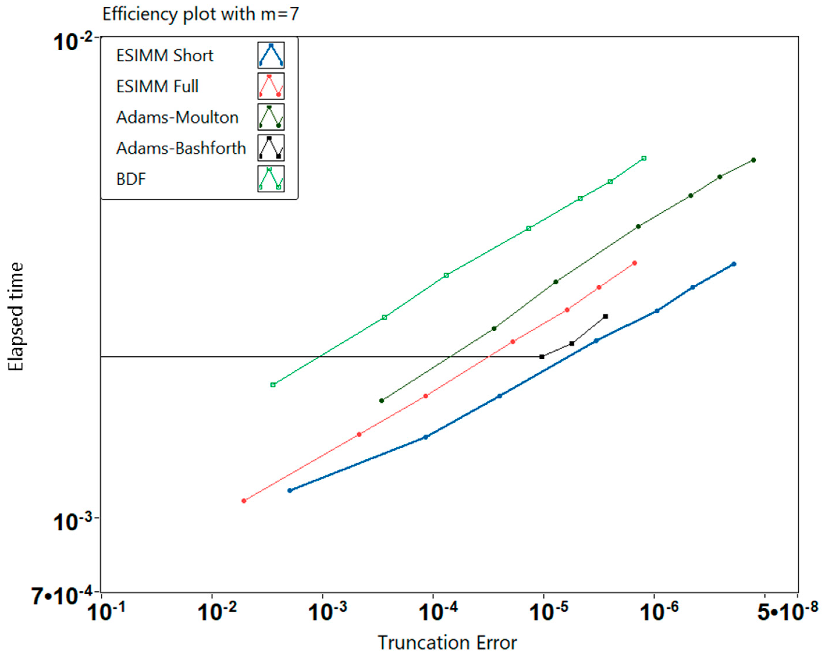
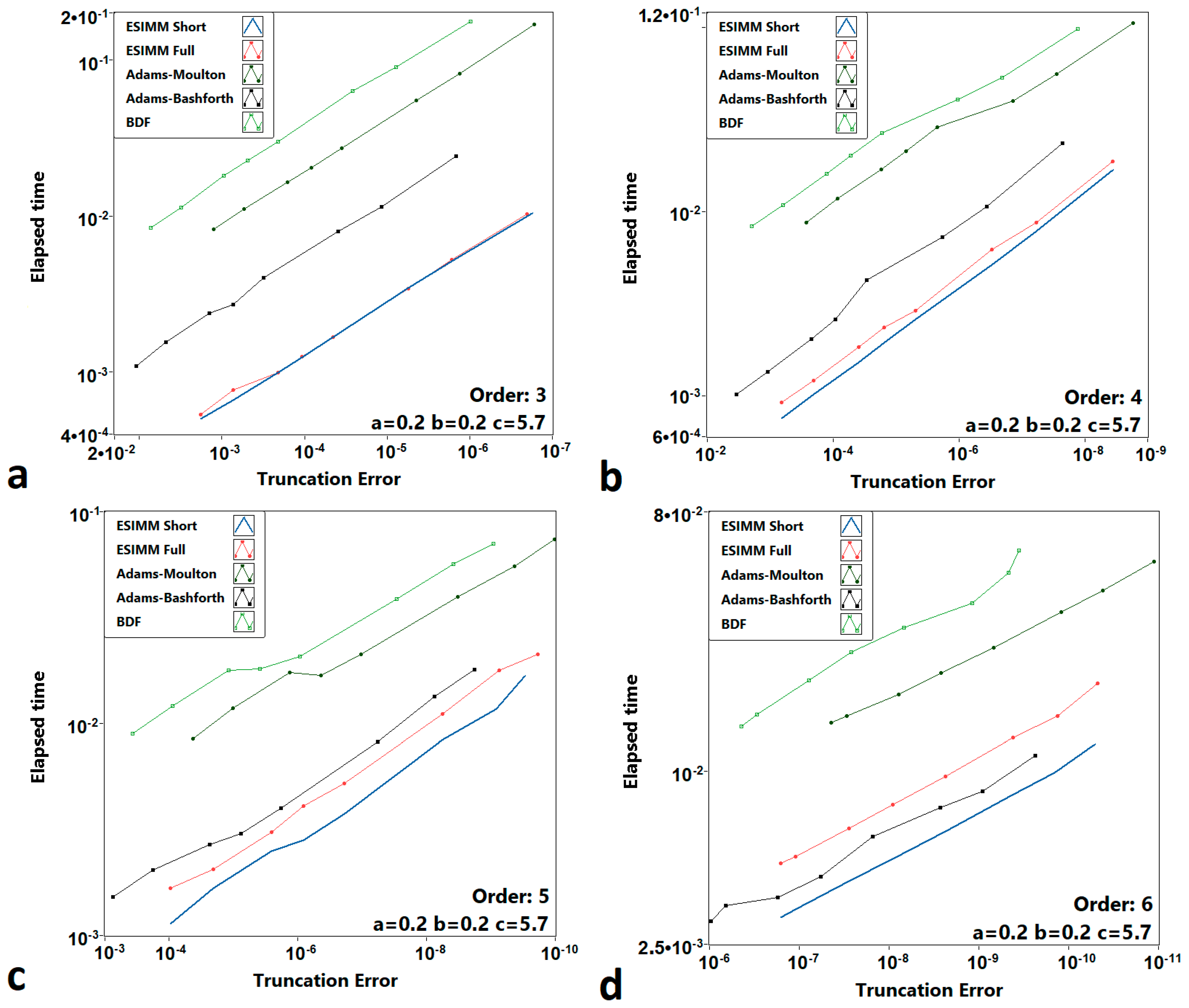
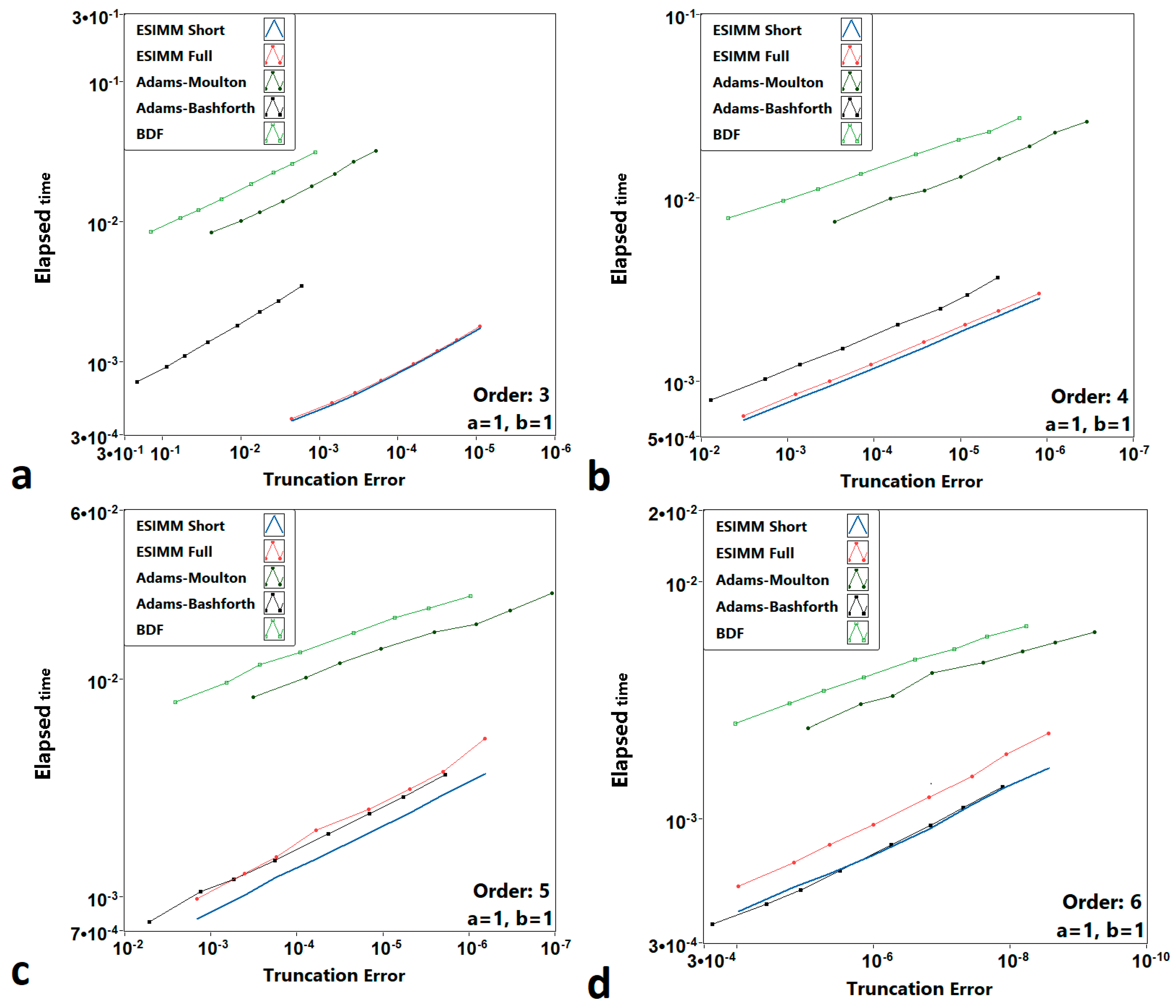
One can see from Figure 3 that the proposed semi-implicit extrapolation multistep method (ESIMM) possesses better performance than well-known linear multistep methods. The “short” version of ESIMM provides a great balance between computational cost and accuracy, while the “full” version is slightly more precise but requires more time to perform calculations. Classical explicit multistep methods such as Adams–Bashforth tend to have closer performance in higher-order schemes but are still significantly less accurate compared to the proposed method.

3.2. Sprott System Case A and Case E

These two systems were proposed by J.C. Sprott in his famous paper [17] and can be written as following initial value problems:

$$\{\begin{array}{l}\frac{dx}{dt}=ay\\ \frac{dy}{dt}=-x+yz\\ \frac{dz}{dt}=b-y^2\end{array}$$

(9)

$$\{\begin{array}{l}\frac{dx}{dt}=yz\\ \frac{dy}{dt}=x^2-y\\ \frac{dz}{dt}=d-4x\end{array}$$

(10)

Sprott Case A is a conservative chaotic system and exhibits chaotic behavior with parameter values a = 1, b = 1. The basic semi-implicit symmetric algorithm for the Sprott Case A system is as follows:

$$x^{n+0.5}=x^n+\frac{h}{2}\ast \left(a\ast y^n\right)$$

$$y^{n+0.5}=y^n+\frac{h}{2}\ast \left(y^n\ast z^n-x^{n+0.5}\right)$$

$$z^{n+1}=z^n+h\left(b-y^{n+0.5}\ast y^{n+0.5}\right)$$

$$y^{n+1}=\frac{y^{n+0.5}-x^{n+0.5}\ast \frac{h}{2}}{1-\frac{h}{2}\ast z^{n+1}}$$

$$x^{n+1}=x^{n+0.5}+\frac{h}{2}\ast \left(a\ast y^{n+1}\right)$$

The semi-implicit basic method for the Sprott Case E system can be written as:

$$x^{n+0.5}=x^n+\frac{h}{2}\ast \left(y^n\ast z^n\right)$$

$$y^{n+0.5}=y^n+\frac{h}{2}\ast \left(x^{n+0.5}\ast x^{n+0.5}-y^n\right)$$

$$z^{n+1}=z^n+h\left(d-4\ast x^{n+0.5}\right)$$

$$y^{n+1}=\frac{y^{n+0.5}+\frac{h}{2}\ast \left(x^{n+0.5}\ast x^{n+0.5}\right)}{1+\frac{h}{2}}$$

$$x^{n+1}=x^{n+0.5}+\frac{h}{2}\ast \left(y^{n+1}\ast z^{n+1}\right)$$

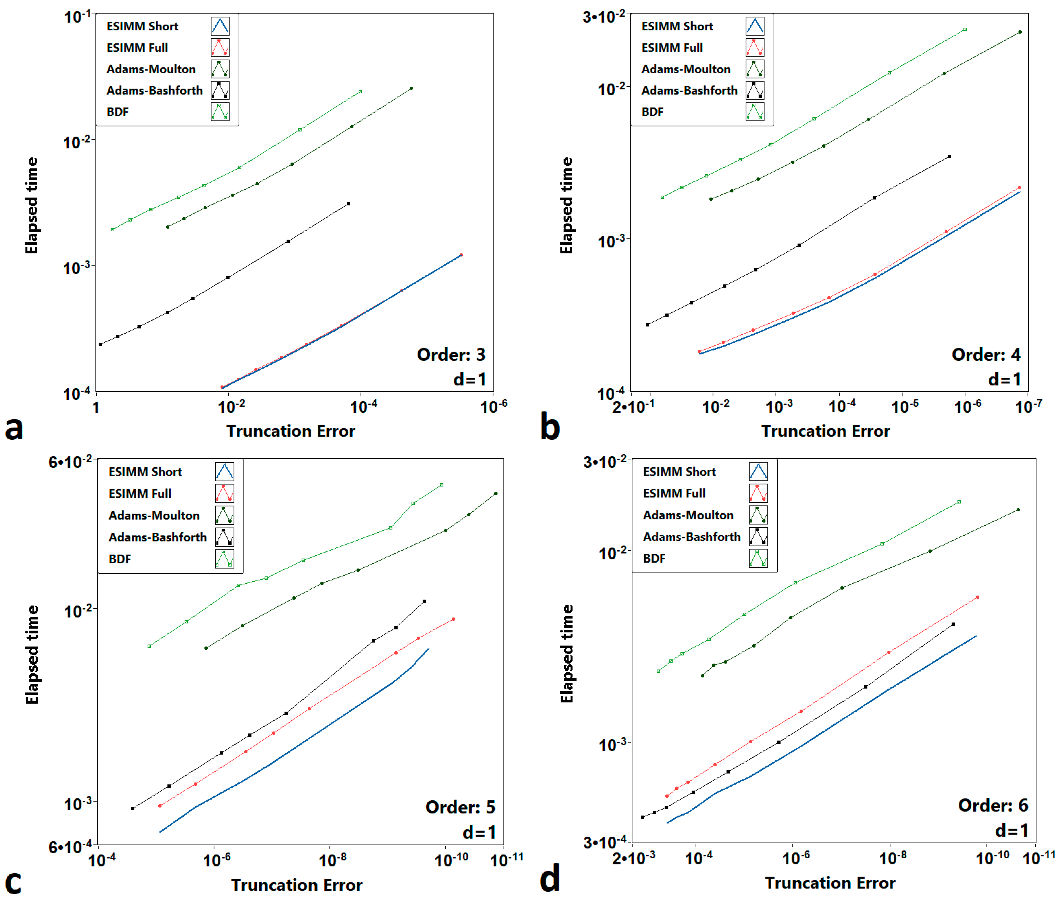
Parameter value d = 11 corresponds to the chaotic regime of oscillations. Figure 4 represents the performance analysis for all investigated methods including the proposed ESIMM algorithms.

The rest of the parameters used to perform the numerical experiments with the system (9) are given in

Table 4. Parameters used in experiments with the Sprott Case A system.

Order	3	4	5	6
Step values, sec.	0.04
	0.03
	0.025
	0.02
	0.015
	0.012
	0.01
	0.008
Initial conditions	(1; 1; 1)
Number of code runs	55

. One can see from Figure 4 that the performance of the ESIMM methods in the case of the conservative chaotic system Sprott Case A was unexpectedly lower despite the symmetry of the underlying basic semi-implicit method.

Thus, the numerical efficiency of the ESIMM algorithm decreases with the increase in accuracy order due to the one extra calculation of RHS function per order, unlike classical multistep methods.

The simulation of the Sprott Case E system confirmed the preliminary results. One can see from Figure 5 that the performance gain of ESIMM methods over the Adams–Bashforth method decreases as the order of the scheme increases. However, the overall results are inspiring due to the known fact that the application of Adams–Bashforth method with orders of accuracy 6 and higher is rare due to the stability issues.

Table 5. Parameters used in experiments with the Sprott Case E system.

Order	3	4	5	6
Step values, sec.	0.085		0.02	0.06
	0.07		0.015	0.055
	0.055		0.01	0.05
	0.04		0.008	0.04
	0.03		0.006	0.03
	0.02		0.003	0.02
	0.01		0.0025	0.01
	0.005		0.002	0.005
Parameter d value	1
Initial conditions	(1; 0; −2)
Simulation time, sec.	30
Number of code runs	40

gives some information on the simulation parameters.

By analyzing results shown in Figure 4 and Figure 5, one can conclude that the semi-implicit ESIMM methods perform well with both conservative (Sprott case A) and dissipative (Sprott case E) systems. They are significantly faster than all other listed methods and give us a rather accurate representation of systems behavior. However, implicit multistep methods such as Adams–Moulton can be more accurate than ESIMM in higher-order schemes, but the proposed method proposes the best trade-off between precision and simulation time, which is extremely important in long-term simulations. To investigate the impact of stiffness on the investigated methods, we additionally considered one more system that is well known as a testbench for numerical integration methods.

3.3. Van der Pol System

This classical nonlinear oscillator was proposed by Balthasar van der Pol [18] and can be written as the following IVP:

$$\{\begin{array}{l}\frac{dx}{dt}=y\\ \frac{dy}{dt}=m(1-x^2)y-x\end{array}$$

(11)

This system is important for our study because the value of parameter m determines the stiffness of the system. The algorithm of the basic symmetric CD method for the system (11) is as follows:

$$y^{n+0.5}=y^n+\frac{h}{2}\ast \left(m\ast \left(1-x^n\ast x^n\right)\ast y^n-x^n\right)$$

$$x^{n+1}=x^n+h\ast y^{n+0.5}$$

$$y^{n+1}=\frac{y^{n+0.5}-\frac{h}{2}\ast x^{n+1}}{1-\frac{h}{2}\ast m\ast \left(1-x^{n+1}\ast x^{n+1}\right)}$$

The simulation parameters are given in

Table 6. The parameters used for experiments with the van der Pol system.

Order	3	4	5	6
Step values	0.02		0.01	0.01
	0.015		0.008	0.008
	0.01		0.007	0.007
	0.008		0.006	0.006
	0.006		0.005	0.0055
	0.005		0.0045	0.005
	0.0045		0.004	0.0045
	0.004		0.0035	0.004
Parameter value	1		0.5
Initial conditions	(1; 0)		(5; 3)	(2; 1)
Simulation time, sec.	30
Number of code runs	40

. The parameter m initially was set to 1, but for higher-order schemes we reduced it to 0.5 to avoid the loss of stability of explicit methods.

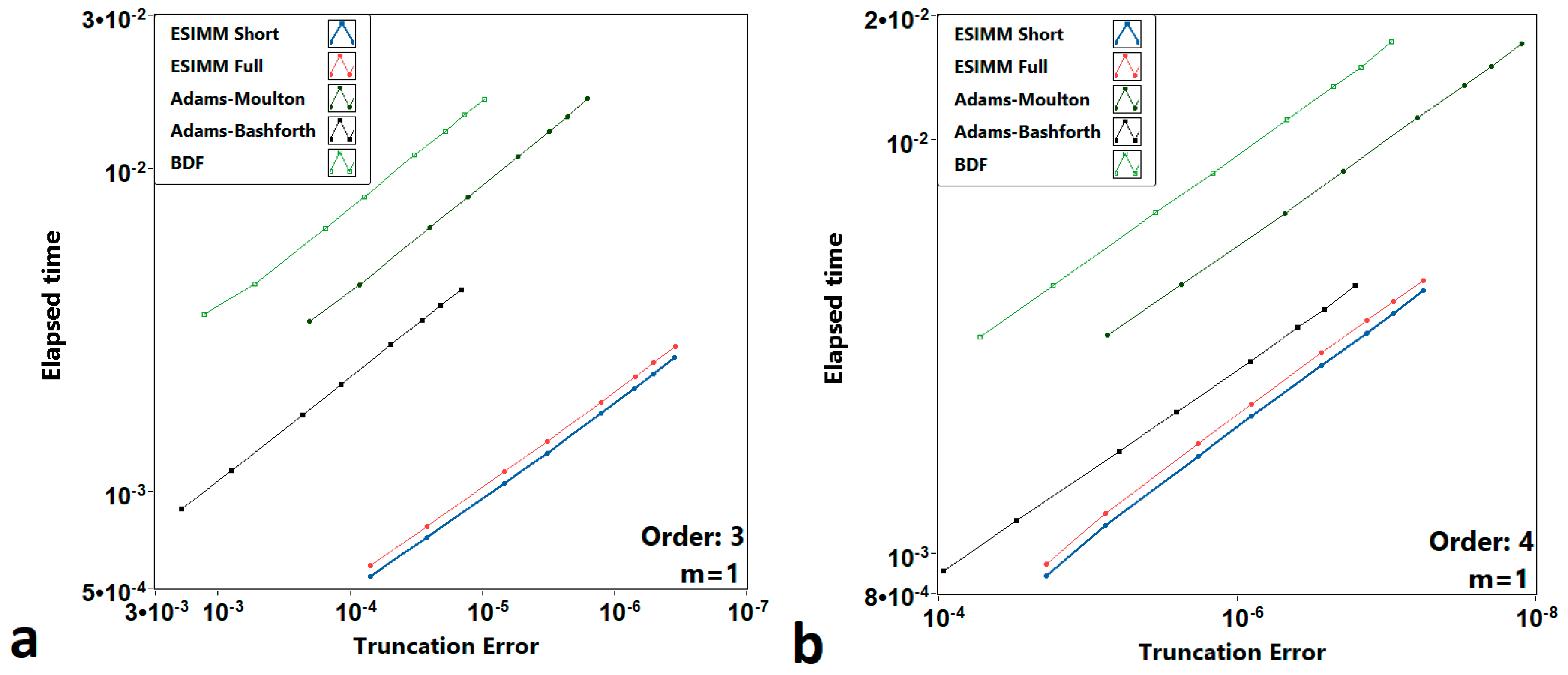
We varied the initial conditions during the experiments to ensure that they do not significantly affect the obtained results. The performance plots for the van der Pol system are shown in Figure 6.

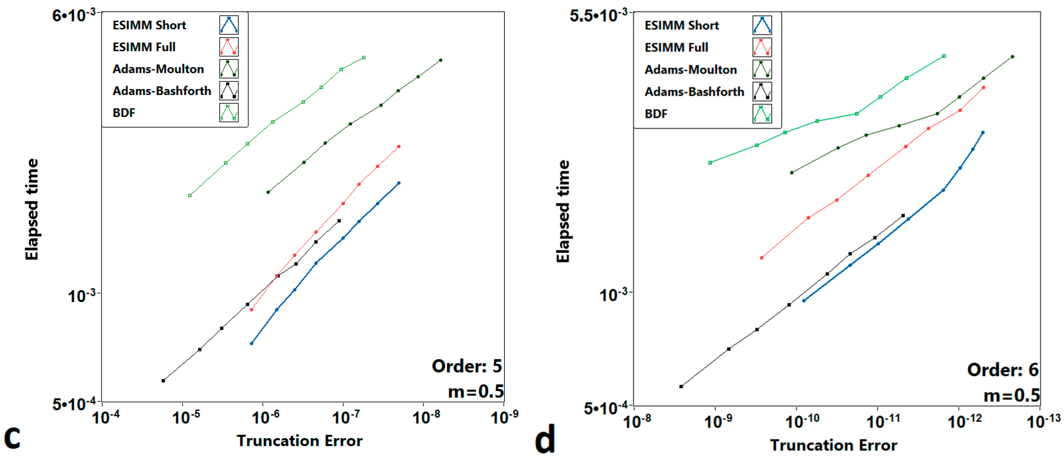
One can see from Figure 6 that implicit linear multistep methods are slightly more accurate than other considered algorithms. Explicit methods such as Adams–Bashforth are, on the other hand, as fast as semi-implicit ones but they lose their accuracy due to less numerical stability. Further increase in m leads to total stability loss for Adams–Bashforth methods. We illustrated this in the final experiment with this system, the results of which are shown in Figure 7. One can see the higher stability of semi-implicit multistep methods in comparison with their well-known explicit counterparts. However, the Adams–Moulton method appears to be the most precise among the investigated algorithms, but the “short” version of the ESIMM solver generally outperforms it due to lower computational costs.

4. Stability Analysis

4.1. Order Plots and Convergence Test

To experimentally evaluate the convergence of the methods under investigation, we applied the approach known as order plots. This type of analysis involves the definition of global truncation error for a numerical method of order N, which can be generally described as E = O (h) ^N, where O is a system-dependent constant and h is integration stepsize [19]. In our experiment, the truncation error was estimated numerically through the simulation of the Rossler nonlinear oscillator by all methods under investigation with stepsize h and h/2. Then, order plots can be constructed as E(h)/E (h/2) vs. stepsize h. An order plot for an “ideal” numerical method of accuracy order 4 should be a horizontal line equal to 16, or for order 5 equal to 32, etc. Thus, the investigated finite-difference scheme can be considered more stable if its order plot is situated higher on the Y-axis and converges faster to the “ideal” line while stepsize decreases. One should note that this method evaluates the convergence and order preservation only empirically and for a certain test problem. We used the 2-norm of maximum truncation errors of all state variables of the system to estimate E(h) and E(h/2).

Figure 8 and Figure 9 show the order plots for all investigated solvers of order 4 and 5, respectively. We omitted the plot for the “full” ESIMM method because it possesses minimal differences from the “short” version in this experiment. One can see from Figure 8 that the proposed method outperforms both explicit and implicit linear multistep methods on the Rossler problem, being closer to the ideal method of order 4 (E(h)/E(h/2) = 16). Figure 9 represents real order evaluation for multistep methods of order 5. The left-hand part of the order plot can be used to roughly evaluate the convergence empirically. One can see that the ESIMM method quickly converges to the “ideal” order 5 (E(h)/E(h/2) = 32) while stepsize decreases. Other methods under investigation show similar convergence, but the explicit Adams–Bashforth method loses stability at a certain stepsize value. Thus, we can conclude that the proposed semi-implicit extrapolation methods can be more stable than explicit linear multistep methods, and possess higher practical order of accuracy for a given set of problems. This confirms the theoretically predicted properties of such methods. However, the analytical investigation of numerical stability is still needed, including the plotting of stability regions.

4.2. Stability Regions

To analytically evaluate the stability of ESIMM methods we will use a technique based on the known approach with 2-dimensional test problems [11,20]. Let us recall that the semi-implicit methods exist only for the initial value problems of dimension 2 or greater, and one needs a special technique here. Consider a 2-dimensional autonomous test problem

$$\dot{x}=Ax, A=\left(\begin{array}{cc}a& b\\ c& d\end{array}\right).$$

Let eigenvalues of the matrix $A$ be

$${\lambda }_{12}=\sigma \pm j\omega .$$

Then, the contents of the matrix can be determined by two free parameters, denote them $r\ge 0$ (eccentricity coefficient) and $k\ge 0$ (asymmetry coefficient):

$$\begin{array}{c} a=kd,\\ b=rc,\\ c=-\sqrt{\frac{1}{r}\left({\lambda }_1^2-\left(1+k\right)d {\lambda }_1+k d^2\right)}\\ d=\frac{2\sigma }{1+k}.\end{array},$$

The shape of the stability region depends on $k$, reaching its maximal size when $k=1$, which corresponds to the Jordan normal form of the matrix, and minimal size when $k=0$ or $k=\infty$, which corresponds to the Frobenius normal form of the matrix. The stability region for the 2-dimensional problem is the area in the complex plane where the absolute values of complex conjugate eigenvalues of the matrix $R\left(Ah\right)$ are not greater than 1.

Let stability region be $R_h\left(Ah\right)$ for stepsize $h$, $R_{2h}\left(Ah\right)$ for stepsize $2h$, and so on. Then, for the two-dimensional test problem, the $s$-stage multistep semi-implicit method can be written in terms of a shift operator $z:x_{n+s}=z^s{x}_n$ as follows:

$$z^s{x}_0=k_1{R}_h\left(Ah\right)z^{s-1}{x}_0+k_2{R}_{2h}\left(Ah\right)z^{s-2}{x}_0+\dots +k_s{R}_{sh}\left(Ah\right)x_0.$$

(12)

From the recurrence equation (12), implying that $x_0\ne {\left(00\right)}^{\top }$, and denoting the identity matrix as $I$, one can obtain the characteristic equation of the method:

$$\det \left(I{z}^s-k_1{R}_h\left(Ah\right)z^{s-1}-k_2{R}_{2h}\left(Ah\right)z^{s-2}-\dots -k_s{R}_{sh}\left(Ah\right)\right)=0.$$

Then, the stability region of the ESIMM method is a region where the maximal absolute value of the root $z_{max}$ of the characteristic polynomial $\det \left(I{z}^s-k_1{R}_h\left(Ah\right)z^{s-1}-\dots -k_s{R}_{sh}\left(Ah\right)\right)$ satisfies the condition $\left|z_{max}\right|\le 1$.

Stability regions of “full” and “short” ESIMM methods are almost the same and are given in Figure 10 and Figure 11. For comparison, we provide stability regions of explicit Adams-Bashforth and implicit Adams-Moulton linear multistep methods as Figure 12 and Figure 13, respectively.

Observing the results of stability analysis, one can see that theoretically predicted properties of the ESIMM methods and the results of the order plot analysis were successfully confirmed. ESIMM methods possess numerical stability that is comparable with implicit Adams-Moulton methods and is far superior to the stability of explicit Adams-Bashforth methods. Despite the fact that the numerical stability of semi-implicit methods strongly depends on the symmetry of the investigated system, we can declare that even in a worth case (full asymmetry of the simulated system) their stability is better than the stability of explicit linear multistep methods which allows implementing these methods with larger stepsizes.

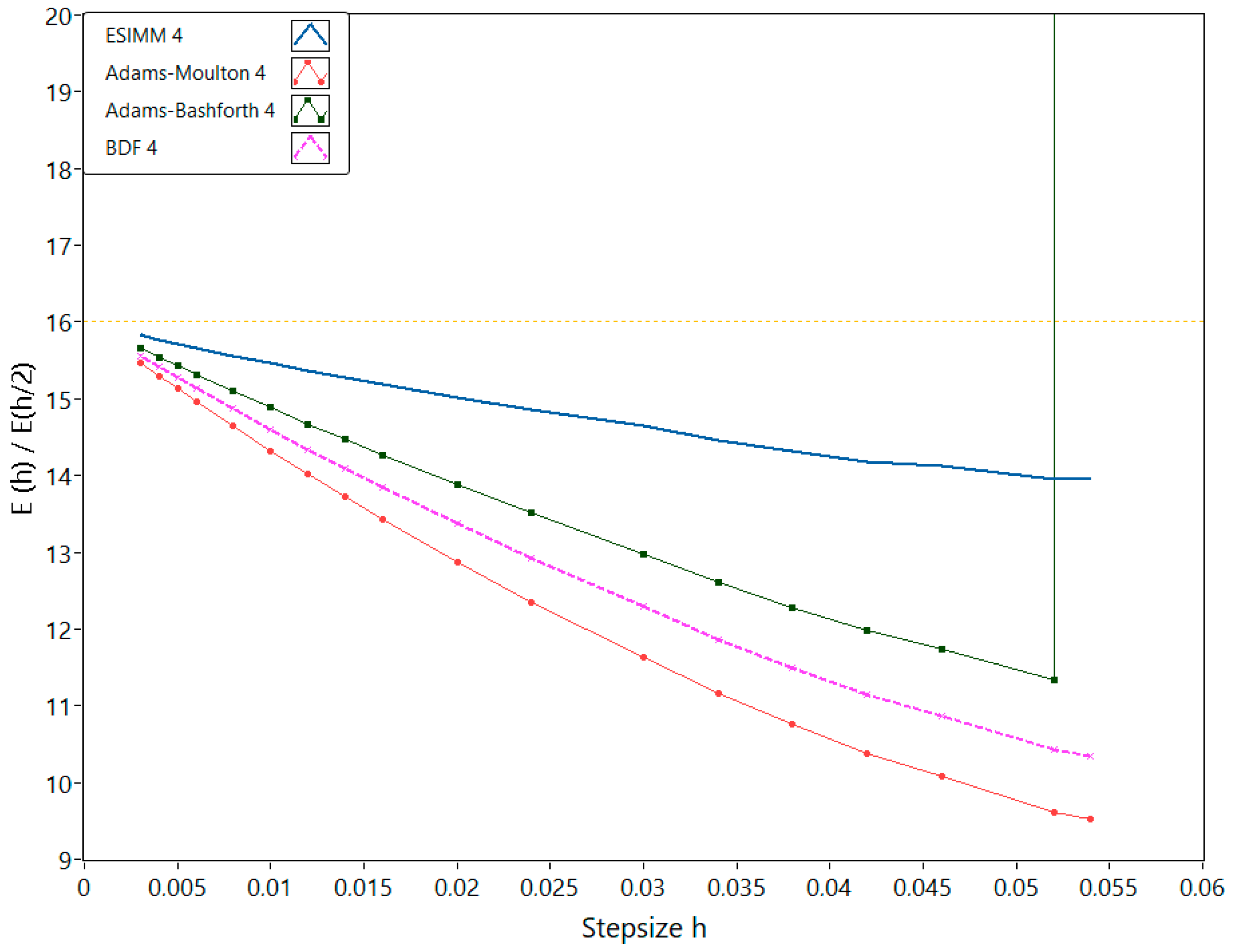
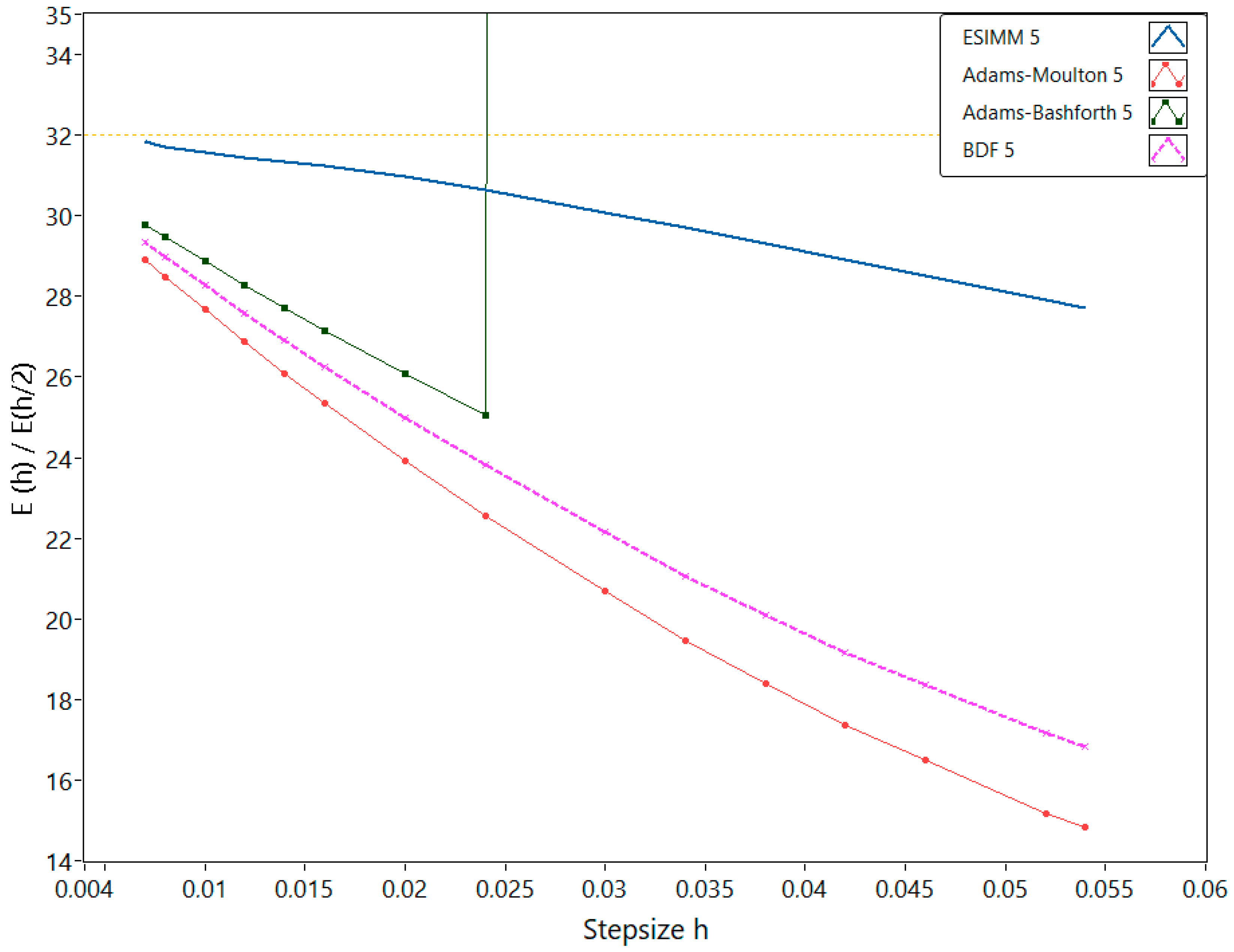
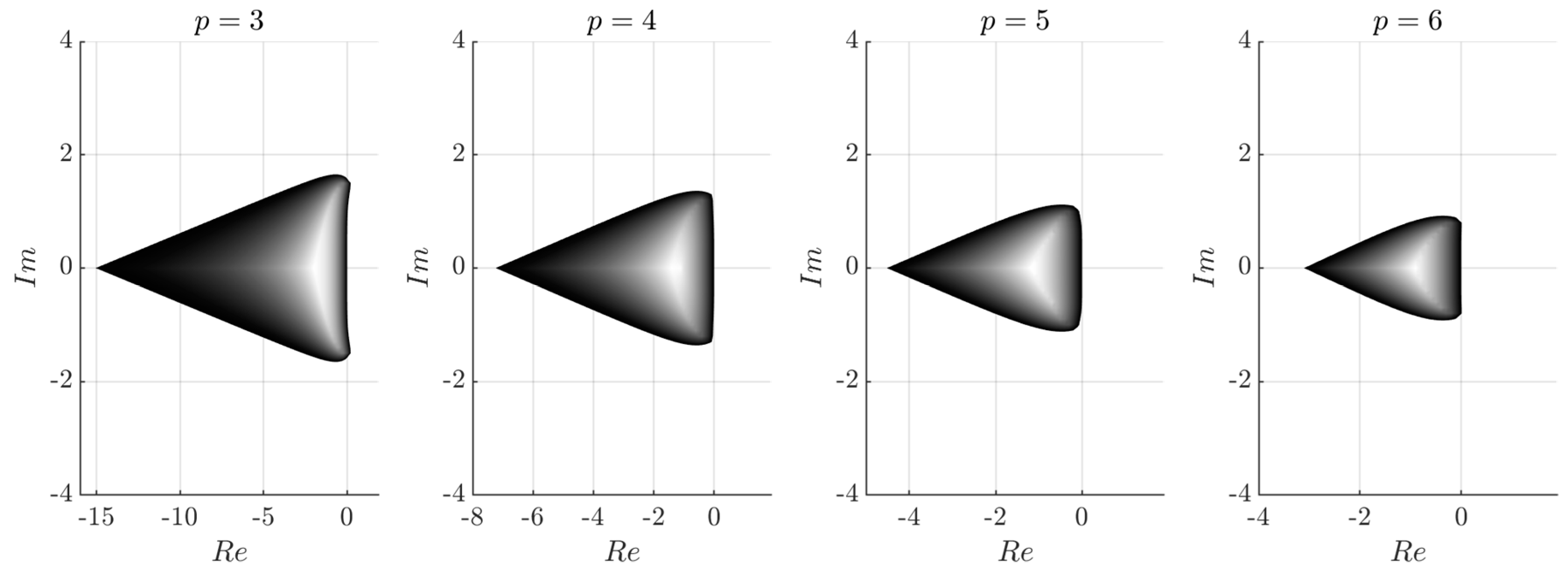
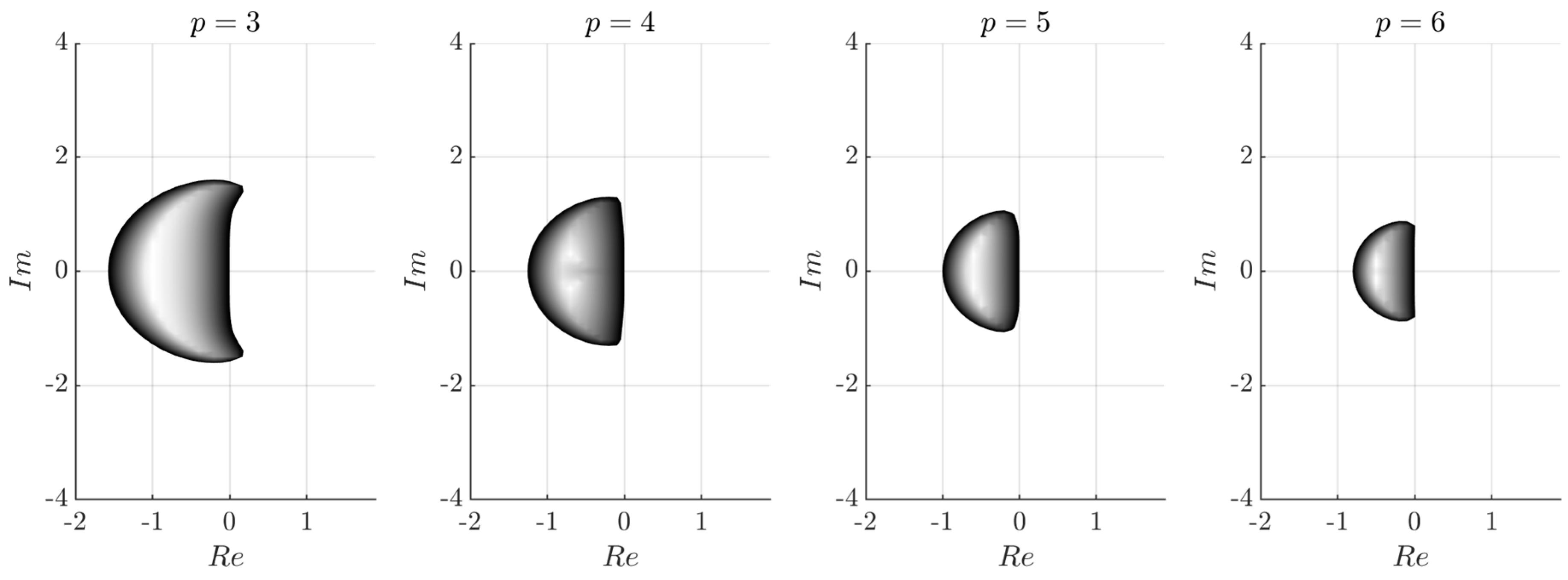
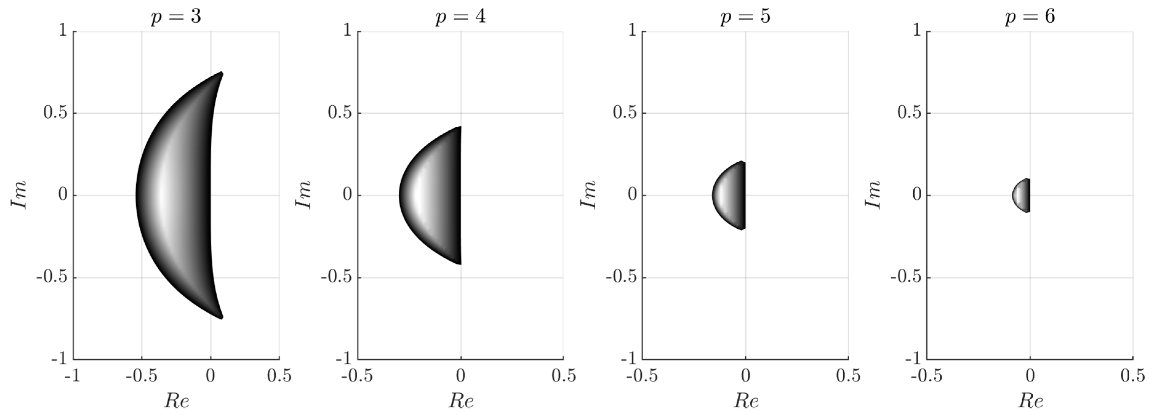
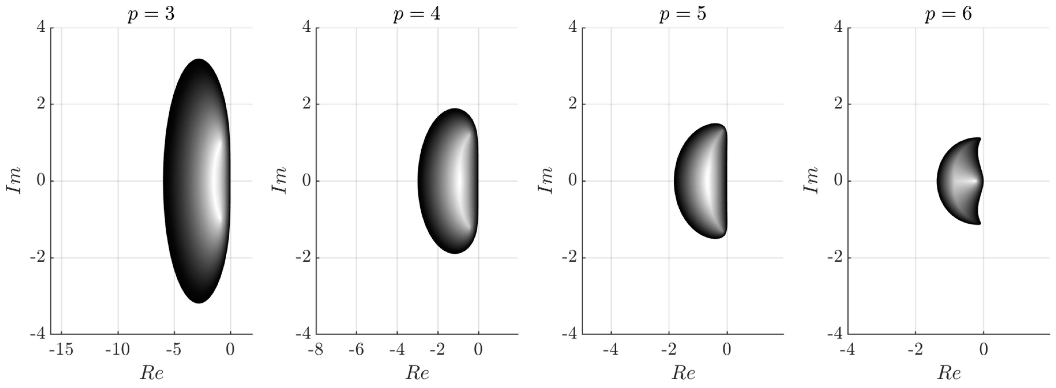
5. Conclusions and Discussion

In this paper, we proposed novel multistep extrapolation methods based on semi-implicit symmetric integration. We explicitly show that the proposed ESIMM integration technique in many cases of nonlinear systems possesses greater performance then well-known multistep ODE solvers. We investigated the order and convergence of the investigated methods experimentally through the order plots using Rossler chaotic system as a testbench. One of the important research questions was the analytical estimation of the numerical stability of ESIMM methods. The investigation of the numerical stability of semi-implicit methods is rather complicated due to their non-trivial call to the right-hand-side function. We used a technique based on second-order linear test problems [11,20] which allowed plotting stability regions for ESIMM and comparing them with stability regions of linear multistep methods.

We explicitly show that the proposed ESIMM solvers are more numerically stable than explicit Adams–Bashforth methods, and, in some cases, implicit Adams-Moulton methods. Moreover, the stepsize range where the order of ESIMM methods preserves, theoretically allows constructing highly efficient multistep extrapolation solvers with adaptive stepsize. Being based on numerical extrapolation, ESIMM methods possess the same capacity to construct built-in estimators of local truncation error as single-step extrapolation solvers. Besides, the ESIMM ODE solvers do not need the concatenation procedure for output data obtained during the starting method and main solution, which also simplifies and fastens the algorithm. The computational cost of the proposed methods was estimated experimentally and is visualized through the performance plots. The program implementation of the proposed methods is significantly simpler than for implicit multistep solvers. Speaking generally, the ESIMM methods are almost as simple as explicit multistep methods, being almost as precise as implicit multistep methods. One of the main drawbacks of the ESIMM method is the necessity to increase the number of basic method calculations by 1 per each increase in the accuracy order. Therefore, high-order solvers, based on the proposed technique, can be less efficient.

In our further studies we plan to implement ESIMM solvers with adaptive stepsize, which requires the development of special step control and coefficient recalculation techniques. ESIMM methods based on other symmetric integrators, e.g., implicit midpoint method or composition solvers [10], are also to be studied.