Abstract
In the present paper, we review the use of two-state, Generalized Auto Regressive Conditionally Heteroskedastic Markovian stochastic processes (MS-GARCH). These show the quantitative model of an active stock trading algorithm in the three main Latin-American stock markets (Brazil, Chile, and Mexico). By backtesting the performance of a U.S. dollar based investor, we found that the use of the Gaussian MS-GARCH leads, in the Brazilian market, to a better performance against a buy and hold strategy (BH). In addition, we found that the use of t-Student MS-ARCH models is preferable in the Chilean market. Lastly, in the Mexican case, we found that is better to use Gaussian time-fixed variance MS models. Their use leads to the best overall performance than the BH portfolio. Our results are of use for practitioners by the fact that MS-GARCH models could be part of quantitative and computer algorithms for active trading in these three stock markets.
1. Introduction
One of the main issues to be addressed in the investment management industry is the proper statistical parameter estimation of the behavior of a return time series (). The seminal work of Markowitz [1,2], the foundational ground of classical Financial Economics, suggests the need of two parameters for security selection: (1) the expected return of the investor and (2) the expected risk exposure. In order to measure the expected return, usually the arithmetic (), exponential, or conditional mean is used, and several approaches have been proposed for this purpose. As an example, there is a wide literature review [3,4,5,6] about the use of factor models in which the value of another variable (such as a market index, a statistical, a financial, or an Economic indicator) determines the value of the expected mean. Other extensions are the use of time series models such as the ARMA (Auto Regressive Moving Average) one.
In this model, it is not assumed that the stochastic process of a return time series () is determined by an stationary, normally distributed stochastic process () with time-fixed mean () and variance (). In this process, depends on past realizations or lagged values (first term in (1) or AR term) and past realizations of the residuals () of the MA model estimated with the second term in Equation (1).
Following the modelling of the expected return with either an arithmetic mean () or an AutoRegressive Moving Average models-ARMA model, the novel proposal of Engle [7] and Bollerslev [8] lead to measure the risk exposure (variance) as a time-varying parameter. This led to the widespread use of the Generalized Auto Regressive Conditional Heteroscedasticity (GARCH) models.
In the previous expression, the value of the variance at , is determined by the past squared values of the residuals () of an arithmetic mean () or an ARMA stochastic process such as Equation (1). The second term in Equation (2) is known as the ARCH term and measures the impact that lagged (or past) realizations of have in the actual variance () value. The third one is a generalization term, known as the GARCH term. This term allows parsimony in the model (a lower number of ARCH terms).
Despite the great breakthroughs and potential uses that the ARMA and GARCH models allow in the financial industry, these have some limitations in their original proposals. They assume that their stochastic process is time-fixed and comes from a single regime. The parameters , , , are the same for all the time series (). This assumption leads to a practical drawback. It is assumed that their values are the same during “normal” and “distress” time periods in the financial markets. If we estimate or (1) for a given financial time series (e.g., the historical returns of a stock index), it is assumed that the value of or the parameters in Equation (1) will be the same. This occurs during normal time periods (such as the 2003–2007 in the main stock markets) and also during distressing periods (years 2007 to 2009).
Given the observed performance in the stock markets, this is not true during these two-time intervals or regimes. During the first regime (a “normal” one or ), the analyst could have measured an expected value and another one in the distressed interval (). This lead us to assume lower expected return values during the distressing time periods than during the normal ones (). In a similar fashion, the analyst could expect that the volatility values (either with a time-fixed or GARCH variance) in the distress time period are higher than in the normal ones ().
Another drawback of the GARCH process in Equation (3) is the fact that the sum of leads to a concept known as “persistence.” This means that, if , there could be misleading estimations of and the analyst could over or underestimate its value. One theoretical cause for this persistence, as some authors suggest [9,10,11,12,13], is the fact that the behavior of the stochastic comes from a multimodal probability density function (pdf). This means that the studied time series has structural breaks, which leads to regimes or states of nature in the behavior of .
For this reason and departing from the seminal work of Hamilton [14,15,16], the expected return () and risk () can be modelled in an S-state of the Gaussian or t-Student stochastic process. This follows for an arithmetic mean () or for the ARMA model.
For the sake of simplicity in our review, we will assume that the return time series of a given stock index follows the stochastic processes given in Equations (3) and (4). We will use the arithmetic mean as a location parameter by following the original practice of Markowitz [1,2]. This sets aside the use of ARMA models to search for the most appropriate ARMA equation. This, in order to avoid more complexity in our estimations. This leaves, for further research, the use of other time series models such as ARMA. This will lead to a parameter set () of two to three parameters in each regime in which are the degrees of freedom of the t-Student pdf for each regime.
In order to estimate the parameter set , the analyst must know which realization in are generated with the stochastic process of each regime. For the sake of simplicity in the exposition as one of our main assumptions, we will model the stochastic process of with two regimes. One regime () for the “normal” or “good performing” time periods and another () for the “distress”, “crisis”, or “bad performing” ones. We used this assumption because we are interested in simplifying the analysis using the two previously mentioned regimes. Additionally, we want to use only two regimes because we want to extend the current literature on Markov-Switching in stock index trading. Practically all these references, as we will mention in the next section, test the use of only two regimes. Lastly, we use a two-regime context by the fact that two regimes, in terms of market volatility or distress, are more easy to follow by the common. It is easier to follow the idea of a low and high volatility (normal or distress) context than a low, high volatility and extra high volatility one.
Given this, the analyst or stock trader must know the regime at . Unfortunately, the regime is not observable, given the time series as the only input data. For this reason, Hamilton [14,15,16] suggests that the unobserved regime at could also be modeled as a time series stochastic process in which the values of are modelled through an -state hidden Markovian chain. With this assumption, the analyst can estimate the smoothed probability () of being in the regime at , along with the transition probability matrix (). This matrix summarizes the likelihood of changing from one regime at , to another at t. We present the two-regime representation of this matrix next:
Now, the use of the Markov-Switching (MS) model extends the probability set () with the addition of the smoothed probabilities of being in each regime, along with the transition probability matrix .
As noted, the MS models in Equations (3)–(6) assume that the variance in each regime () is time fixed. This issue has an important implication because, even in each regime, the volatility levels could be time varying. If this effect is not taken into account in estimating the parameter set, the analyst could have misleading estimations of the risk exposure () and also the smoothed regime probabilities (). For this reason and as a natural solution to the persistence effect in the GARCH model (2), an ARCH (Markov Switching Component ARCH Model-MS-ARCH) or GARCH (Markov-Switching GARCH Models-MS-GARCH) extension of the MS model was proposed [12,13,17].
Given the features of Markov-Switching models, there are many practical applications of these. The most common one is to characterize the performance of a time series. Additionally, these can be used to measure the contagion (spillover) effect between financial markets and economic indicators in a multiple regime context. Therefore, the characterization or spillover test can be made (in the context of our paper) in a “normal” or low volatility () regime or in a “distress” or high volatility period (). From all the potential uses, we are interested in their use for stock trading decisions.
Given the development of the 2007–2009 Global financial system crisis and its corresponding spillover effect, several investors faced significant losses in their portfolio’s value. Had they had a quantitative model to forecast the probability of being in a distress time period at , they would have rebalanced their equity portfolio into a less risky one.
The rationale of using MS models for investing comes from the pioneering proposal of Brooks and Persand [18]. This work has been extended by Kritzman Page and Turkington [19], Hauptmann et al. [20], Engel, Wahl, and Zagst [21], and De la Torre, Galeana, and Álvarez-García [22]. From all these works, only the last one reviews the use of MS models in a developing stock market (Mexico). The other works study their use in the equity markets of Germany, Switzerland, the U.S., or the U.K.
In a parallel fashion, all the previous papers used the original MS, which is a time-fixed variance model of Hamilton [14,15]. Given this, little has been written about the use of MS-GARCH models in trading algorithms.
Departing from these two issues, we have the main motivation of this paper. This includes performing one of the first tests of using MS-GARCH models in trading algorithms, which are applied in Latin-American stock markets. This comes from a U.S. dollar (USD) based investor perspective. Our intention is to extend the scant literature related to the use of MS models in stock trading. This, to the Latin American case. In addition, we are interested in extending the related literature to the review of MS-GARCH models in stock trading algorithms.
Even if it is possible to incorporate the effect of asymmetric shocks in the time varying GARCH variance, we will present the results of symmetric GARCH variances, along with symmetric Gaussian and t-Student likelihood functions in each regime. We did this because the combination of the homogeneous (same marginal pdf in each regime) and heterogeneous, symmetric, and asymmetric regime probabilities MS-GARCH models could be complex. In addition, presenting the results of homogeneous and heterogeneous variances could be wider in each of the three indexes. In order to expose the benefits of Gaussian or t-Student MS-GARCH models in stock trading, we will assume homogeneous GARCH and regime pdfs. Additionally, we will assume symmetric effects of financial shocks in the GARCH processes. As we will mention in our conclusions, the extension of our results to asymmetric variances and regime pdfs along with heterogeneous regime pdfs and variance processes will be left as a task for further research.
In order to run our review, our simulations (back tests) were made in the three main MSCI Latin America (LATAM) indexes: the MSCI Brazil, Chile, and Mexico stock indexes. We selected these three indexes because these markets showed the Highest Latin America (LATAM) turnover figures of the World Federation of Exchanges [23]. Even if Argentina has one of the most important stock markets in the region, we omitted this country due to its fiscal and economic issues observed in the last three years of our review. In some periods, this country’s stock market was classified as an emerging market and, in some others, as a frontier one [24]. Additionally, the impact of their fiscal and debt negotiation, along with the emerging support of the International Monetary Fund, could lead to a behavior that is notably different from the other three markets.
We simulated the performance that U.S. dollar USD-based investors would have had, had they used our trading algorithm (with MS-GARCH models as a quantitative method). This takes place from 1 January 2000 to 30 January 2019.
Our rationale is that the use of the simulated algorithm with MS-GARCH models leads to better performance against a “buy and hold” strategy in the three main LATAM stock markets.
Our results, as we will observe, could give theoretical support for the use of two-regime MS-GARCH models in stock trading especially if a given practitioner wants to make active trading in the three main Latin-American stock indexes. In addition, we are providing practical evidence about the benefits of MS or MS-GARCH models as the core of a trading algorithm. Lastly, we extend the literature by testing the benefits of time-varying variances in MS-GARCH models.
Given our theoretical and practical motivations, we structured the paper as follows. In Section 2, we discussed the current and most relevant literature about the use of MS and MS-GARCH models. In this review, we made a special emphasis in their little reviewed use in stock trading decisions. In Section 3, we present our back tests’ material and methods. In this case, we present an introductory review of the MS and MS-GARCH models and their use in the trading algorithm. In addition, in that section, we tested the goodness of fit of MS and MS-GARCH models for the regime characterization of the three simulated indexes along with the back test’s pseudo algorithm. In Section 4, we make a review of our simulation results and, in Section 5, we present our conclusions and guidelines for further research.
2. Literature Review of the Use of MS-GARCH Models
Since the original proposal made by Hamilton [14,15,16], MS and MS-GARCH models have been useful to characterize the behavior of a time series in separate regimes. As mentioned in the previous section, this model allows us to estimate their corresponding location (usually mean, ) and scale (variance or standard deviation, ) parameters. Additionally, by treating these regimes as an unobserved first order Markovian process, MS and MS-GARCH models are useful for estimating several output parameters. One of these is the probability of being in each regime at and the transition probabilities given in Equation (5). Departing from the output parameter set of MS and MS-GARCH models, several potential applications were tested in economics and finance.
As examples of their applications in time series modelling and crisis spillover measurement, we can mention the work of Ang and Bekaert [25,26], Kritzman, Page and Turkington [19], Klein [27], Areal, Cortez and Silva [28], Zheng and Zuo [29], and Hauptmann et al. [20]. These papers determine the appropriateness of MS models to characterize the time series of developed financial stock markets (the U.S., the U.K., Germany, France, Switzerland, or Japan). They do this with the presence of either two or three regimes. In addition, the works of Alexander and Kaeck [30], Castellano and Scacia [31], and Ma, Deng, and Ho [32] study the benefit of using MS models in the time series of credit default swaps (CDS) and the contagion that their performance have in some other markets, such as the oil ones.
As a practical and useful application, MS models are currently used to predict the probability that the U.S. could be in recession [33]. This use is based on the original paper of Chauvet [34] who suggested performing a two-regime MS regression of the U.S. Economic cycles with four coincident indicators: (1) the non-farm payroll employment, (2) the index of industrial production, (3) the real personal income (without transfer payments), and (4) the real manufacturing and trade sales. The paper shows evidence about the benefit of MS models to forecast recession time periods. This is an analogue used to the warning system with which our simulated trader will decide whether to invest in a stock index in normal or distress periods.
For the specific application of MS models in Emerging financial stock markets, we can mention the papers of Ma, Deng, and Ho [32], Riedel and Sottile [35], and Riedel, Thuraisamy, and Wagner [36]. These three works test the use of MS models in emerging economies’ CDS or credit markets. Similar to the previous authors who test the impact of CDS rates in developed stock markets, these papers also find a relation and spillover effect between the CDS markets of the studied economies and their corresponding stock or money markets.
In a similar fashion, the works of Zhao [37], Walid et al. [38], Walid and Duc Khuong [39], and Rotta and Valls-Pereira [40] discuss the link between the volatility of emerging countries’ stock markets and their corresponding currency pairs against the U.S. dollar. In the three works, the authors found a link between these two types of markets in the BRIC (Brazil, Russia, India, and China) region with a more observable two-way contagion effect during the high volatility regime ().
Another interesting review of the MS model use is the spillover of currency crises between integrated regions such as the European one. This is done, given the impact of monetary policy changes. Among the papers that address this issue in developed markets, we found the work of Mouratidis et al. [41], Miles and Vijverberg [42], and Lopes and Nunes [43]. These authors found the change in the inflation or monetary policy has a significant impact on the probability of the distress regime of the studied currencies.
In the study of the previously mentioned issue in emerging economies, we found the papers of Kanas [44], Álvarez-Plata and Schrooten [45], Parikakis and Merika [46], Girdzijauskas [47], Dubinskas and Stungurienė [48], Kutty [49], and Ahmed et al. [50]. These authors found a close relation between the changes in expectations in the interest target rate and the performance of the studied emerging markets’ currencies or stock markets. In addition, Dufrénot, Mignon, and Péguin-Feissolle [51] found evidence of a spillover effect from the distress probability in the U.S. stock markets to the LATAM ones. Similarly, the work of Sosa, Ortiz, and Cabello [52] shows strong proof that the influence of the stock markets in its corresponding foreign exchange (FX) rate is strong in Chile, Colombia, Mexico, and Peru.
Even if the works mentioned in the previous paragraphs do not have a direct relationship with our tests, these give strong support for the use of MS and MS-GARCH models against single regime stochastic processes. In addition, these works characterize the MS stochastic process to emerging stock market indexes, such as the ones studied herein.
For the more specific application of MS models in emerging stock markets, we found the work of Cabrera et al. [53] and De la Torre, Álvarez-García, and Galeana-Figueroa [54]. These authors tested the use of MS and MS-GARCH models to characterize the performance of the main indexes of Bolivia, Brazil, Chile, Colombia, Mexico, Peru, Venezuela, and the MSCI LATAM index. This occurs along with the review of the U.S. S&P500 index. In their results, these two works show strong evidence in favor of the characterization of these stock indexes with two or three regimes. The paper of Cabrera et al. [53] found that it is preferable to use MS-GARCH models to characterize the stock indexes of these countries (a result in line with ours in this paper). In addition, the authors search for evidence in favor of a potential LATAM common distress cycle, but only Chile and Mexico show this behavior with the U.S. This last paper is one of the main motivations of ours and led us to test the use of MS-GARCH models for trading decisions in these three LATAM stock indexes.
All the previous literature makes a punctual and elegant review of the use of MS and MS-GARCH models in finance or economics. Despite this, none of these deal directly with the subject of using these models for trading.
The first work that propose the use of Gaussian MS models for trading is the one of Brooks and Persand [18]. It is the main theoretical motivation and departing point in this paper. In their work, the authors suggest the estimation of an MS model in the equity/bond yield ratio of the U.K. FTSE100 index and the 10-year Gilt. The rationale of their investment strategy is a very straightforward one: to invest in the U.K. Gilt and the FTSE100, given the smoothed probabilities of being in each regime at . Therefore, the investment level in each asset is given by the next expression.
With these trading weights, it is expected to invest more in the equity market in the normal time regime and less in the “risk-free” gilt. If the probability of being in the distress period is higher, it is expected to invest more in the U.K. gilt and less in the FTSE100 index. With the assumption of no trading costs, the authors found strong proofs in favor of using the MS model for active trading. This occurs against a “buy and hold” investment strategy in the FTSE100 or the 10-year U.K. Gilts. This work, as previously mentioned, is the departing theoretical point of our research. The difference between this paper and our tests is that, instead of using the smoothed probabilities as weights, we used these to decide whether to invest fully in the stock index. That is, we decided whether to invest all the portfolio proceedings in the stock index during normal periods or to do it in the risk-free asset during distressful periods.
In a similar manner to Brooks and Persand [18], Ang and Bekaert [25,26] extend the use of MS models to estimate MS covariances. With these, the authors simulated the performance that a USD-based investor would have had, had she made an international diversification in Germany, Japan, the U.K., and a European index. In their results, the authors found strong proof of a correlation clustering during distressful periods and a reduction in the diversification benefits. Given this result, they simulated the performance of an optimal portfolio in which the used regime-specific covariance matrix change, given the probability of being in a normal or distress period. Their results suggest that it is preferable to use an MS portfolio strategy than a passive or buy and hold one. This paper motivates the current one by the fact that the authors prove that the practice of rebalancing a portfolio in distress or the crisis time periods leads to an over performance against a buy-and-hold strategy.
With a similar portfolio perspective and a similar theoretical motivation to the present one, Kritzman, Page, and Turkington [19] suggest using the Baum and Welch [55] algorithm to perform a more computationally efficient estimation of the MS model. These authors use their proposed method for estimating the expected return vector of a multi-asset portfolio diversified with equities, strategy indexes, and financial risk factors. From a starting base portfolio, they suggest a series of tilts, given the smoothed probability of a distress time period in the stock market. They also incorporated (in the tilt decision) the probability of recession and the likelihood of a high inflation episode. Their simulations also show the benefit of using MS models for active investment.
Following these works, we found ones of Hauptmann et al. [20] and Engel, Wahl, and Zagst [21]. In these papers, the authors develop a warning system for the S&P 500, the Eurostoxx 50, and the Nikkei 225 stock indexes. In their proposal, the authors estimate a Gaussian three-regime model for the stock index and then use several economic and financial risk factors to estimate a logit warning system. This led to estimating time-varying smoothed regime probabilities and time-varying transition probabilities. In their review, the authors tested the performance of the S&P 500 index with a similar “tilt” investment strategy as the one of Kritzman, Page, and Turkington [19]. Their results show, as appropriate, the use of their warning system.
In a parallel test, Engel, Wahl, and Zagst [21] simulated, without the impact of transaction costs, the performance of an equally weighted portfolio of the S&P500, the Eurostoxx 50, and the Nikkei 250. This is a similar investment strategy to Hauptmann et al. [20]. Compared to the case of the previous works, their simulated portfolio also outperformed the corresponding passive investment strategy.
Lastly, we found the work of De la Torre, Galeana, and Álvarez-García [22] that test the use of MS models in the U.S., U.K., Italian, and Mexican stock markets. These authors simulated an agent that invested in stocks (risk-free asset) during normal (distress) time period at . With weekly simulations that include the impact of trading costs, they found that the use of Gaussian two-regime MS models leads to alpha generation. For the specific Italian case, they found that the accumulated return in the simulations was negative. Despite this outcome, the result is better than the observed one in the corresponding passive strategy. The present paper has the intention of extending the review in the Mexican market by using Gaussian and t-Student MS-GARCH models in the trading decision algorithm.
Given our literature review and, as noted, little has been written about the use of MS models for investment decisions. Related to this use, we found two type of reviews in developed stock markets.
- A two-asset trading algorithm that determines in which asset to invest, given the probability of being in each regime at or .
- A portfolio management system, in which some tilts in the investment weights are made, given the same probabilities.
From the previously mentioned strategies, we want to extend use of the first type of strategy. Given our literature review and research interest, we found no literature that test the benefits of a two-asset strategy in the main LATAM markets. This uses a U.S. dollar (USD) based investor perspective. Additionally, we found that only the work of Engel, Wahl, and Zagst [21] use time-varying MS-GARCH models and these are used in developed stock markets.
Given this, we tested the performance of a USD-based investor that followed the next trading rule in the three main Latin America stock markets.
- To invest in the simulated stock market index if the investor expects to be in the low volatility () regime at or
- To invest in the U.S. risk-free asset if the investor expects to be in the high volatility () regime.
Once our theoretical motivations were mentioned, we presented a brief review of the rationale behind the MS-GARCH model. We do this section for introductory purposes and also to explain how we used the MS and MS-GARCH models in the investment strategy.
3. Backtest Materials and Methods
3.1. The MS-GARCH Model and Its Use in the Active Trading Algorithm
The MS-GARCH model that we will test herein has the functional form of (10). As Haas, Mitnik, and Paolella [13] suggest, the MS-GARCH models must be inferred once the residuals have been calculated from a conditional mean such as the one of an arithmetic mean or an ARMA model in . Since this paper is the first test of the application of the MS-GARCH model for investment purposes in the main LATAM stock markets, we used the arithmetic mean of the returns (we will leave the application of ARMA models for further research). With the residuals determined as , we used these to calculate the MS-GARCH model. We did this by assuming that the stochastic process can be modeled with a two-regime Markovian chain that can be filtered, at , from the time series of . This takes place with either a Gaussian or a standardized t-Student filtered probability function as follows, respectively:
In these expressions, are the degrees of freedom that determine the shape of the t-student pdf. These will lead us to the maximization of the next log-likelihood function, in which is the stable probability (mixing law) of each regime (please refer to Hamilton [14,16] for further reference).
In order to estimate the parameter vector of (10), we will use a maximum likelihood method with the Viterbi [56] algorithm as used in the MSGARCH R package [57]. R and this package are the core computational software of our back tests and trading algorithm. From the inferred parameters with Equations (12) to (14), we were interested in the filtered probability at and the transition probability matrix . With these, we can estimate the probability of being in each regime at as follows.
Given the two forecasted probabilities of being in the regime at , an investor can determine if she expects to be in a high-volatility regime at with the next indicator function.
We propose this regime filtering, given in Equations (12) or (13) by following the standard suggestions in the related econometrics literature [14,15,16,18,19,20,25]. Once the filtered probabilities (12) or (13) were estimated with the Viterbi algorithm, we inferred their smoothed values, given Kim’s method [58].
A natural question of the MS-GARCH model use is: why is it necessary to compare the performance of an investor if using either a MS, MS-ARCH, or MS-GARCH variance in Equations (12) or (13)? Our position is that, given the time-fixed ARCH or GARCH scale parameter used in Equations (12) or (13), the estimated smoothed probability of each regime will differ. This result will also lead to a different precision level in the forecast of . With these different values of , it is expected that there will be different trading decisions in Equation (16) at . Given this, we backtested six scenarios in which we changed the variance estimation method (time-fixed, ARCH, or GARCH) and the Log-Likelihood Function (LLF) function with Equations (12) or (13).
Given the regime expectation in Equation (16), the trading algorithm that we tested herein was translated to the next computational decision system at :
- To invest in the simulated stock market index if the investor has a regime expectation of .
- To invest in the U.S. risk-free asset if the investor has a regime expectation of .
Given the use of MS and MS-GARCH models in this computational trading algorithm, we will proceed to describe the simulation process used.
3.2. Data Description and Markov-Switching Tests
In order to simulate the benefit of investing with the MS trading algorithm in the stock markets of interest, we will assume (as mentioned previously) that the investor is a USD-based one.
Given the description of the MS-GARCH models used in the investment strategy, we will use the USD historical weekly data of the MSCI [24,59] indexes that we present in Table 1. All the time series start at 6 June 1998 and end on 1 February 2019 (a total of 1079 weekly realizations). As we will mention later, we simulated the investment strategy from 1 January 2000 in order to use the previous weeks of data at for estimation purposes.

Table 1.
The Latin American stock indexes that will be used in simulating the investment strategy.
All the time series used in our simulations came from the databases of Refinitiv™ Eikon™-Xenith™ [60]. In order to estimate the MS-GARCH model, we transformed the original price () time series of the six stock market indexes into a return () one. We did this by using the continuous time return calculation. Once we have done this, we had six return time series with a total of 1078 weekly returns each (since January of 1998).
The Statistical performance of this full time series is shown in Table 2. Almost all the six indexes had similar minimum weekly returns in a single week and similar mean weekly returns (with the exception of the Chilean market that has the lowest mean value of 0.15%). In terms of standard deviation, the Chilean index could be interpreted as the safest one (with a weekly standard deviation of 4.9%) and the Brazilian and Mexican markets as the riskiest ones.
Table 2.
Statistical summary of the weekly returns of the three stock indexes studied here (values as percentages).
In the same table, we present the results of the main probability density function (pdf) fiting tests. These include the Gaussian and t-Student Kolmogorov-Smirnov test (a test more focused in the central segment of the pdf), the Anderson-Darling normality test (more focused in the tails), and the skewness and kurtosis levels for the Jarque-Bera one. Given the high kurtosis level, there is no evidence that shows the returns of these three indexes are either gaussian or t-Student. This suggests two possible explanations: (1) we should consider a longer tail pdf such as the Generalized Error Distribution or (2) there is a presence of potential high kurtosis, given the fact that the time series should be modeled with two or more regimes. In this paper, we test the second explanations. Essentially, the return time series can be modelled with a Gaussian or t-Student two-regime pdf. Thus, we observe a high kurtosis level in the entire time series, but this high kurtosis is due to the presence of two regimes (low and high volatility) in the stochastic process. If we model this stochastic process with such a number of regimes (two), it is possible to identify that the pdf in each regime is gaussian or t-Student. For this reason, we will perform the next Markov-Switching model fit tests with information criterions.
Following the statistical summary in Table 2, we determined, with the Akaike [61] Information Criterion (AIC), if it is appropriate to model, with one or two-regimes, the stochastic processes of each index’s return. With the AIC, we also reviewed if it is more appropriate to use a MS-ARCH, a MS-GARCH, or a constant variance MS model (no ARCH and GARCH terms). We also made these comparisons by using either a Gaussian or a t-Student pdf in the estimation process.
We used the AIC instead of other information criterions or other criteria as the Root Mean Squared Error (RMSE) for two reasons.
- The MSGARCH R package [57] can estimate only a GARCH(1,1) variance process. The maximum lag in the ARCH and GARCH terms are 1. Given this, the use of the Schwarz [62] or the Hannan-Quinn [63] one, are not necessary because we only want to determine the most accurate MS or MS-GARCH model (an issue in which the AIC is better than the other two criterions). This computational restriction sets aside the trade-off between accuracy and parsimony in the model.
- We prefer to use an information criterion such as the AIC because we want to test the goodness of fit of the estimated model. For this reason, it is preferable to use the AIC criterion that uses the LLF as input. The value of this function, along with the number of parameters and the length of the time series (information set), could give us more accurate fitting values than the sample RMSE. In addition, since we used the Viterbi [56] algorithm, one of the outputs of the estimation process is the LLF (the value to be optimized in the estimation process). Given this, it is natural for us to use the AIC as a fitting parameter than the RMSE.
Departing from this fitting criteria for our analysis, we present the first fitting results of each index in Table 3.
Table 3.
Summary of fitting the different MS models used as candidates for the stochastic process in each index.
The reader can note that, in all the indexes, the two-regime Markov-Switching are more appropriate to model the stochastic process of each index. From Table 3, it is also noted that the Gaussian MS-GARCH model gives the best fit for the Brazilian and Mexican indexes and that the MS-ARCH (with no GARCH term) gives the best fit for the Chilean case. This test is made on the full time series since 6 June 1998 to 1 February 2019.
Since the previous test applies to the entire time series and, in order to check the robustness of these results, we ran a recursive estimation of each model in each index from 7 January 2000 to 1 February 2019 (996 weeks). For estimation purposes, we used 7 January 2000 as starting date (t = 1), with all the historical time series since January 1998.
Next, in each simulated date , we added the realization of the corresponding week to the information set. This test was useful to determine if the results of Table 3 hold across the time and will be of use in the investment strategy simulation.
In Table 4, we summarized the observed mean value of the weekly AIC for each index in each simulated scenario. The Gaussian time-fixed variance MS model is the best fit, which is a result that contradicts the results of the full time series analysis of Table 3. This is an interesting result because it gives guidelines to note that the use of Markov-Switching models is preferable in the risk modelling of these three indexes. However, in a week-by-week basis, it is preferable to use an MS constant variance instead of an MS ARCH or GARCH one.
Table 4.
Summary of the weekly recursive fitting analysis of the different MS models tested in each index.
A natural question with this estimation method that could arise is: Why did we not use a rolling time window instead of a recursive (length increasing) one? We did not want to use a rolling time window because the estimation method of the MS and MS-GARCH is a Bayesian one. Essentially, we are inferring the parameters of a hidden Markovian process from the observed data (time series). The estimation process is similar to the Kalman filter, as Hamilton [14,16] observed. Our rationale is: if the information set is bigger (the time series is longer), our estimations of the parameter set () are more accurate. In order to use a time rolling window, we must determine the appropriate window length (number of realizations in the time series) and this question is part of parallel but different research efforts. Given this, we prefer to a use recursive, increasing window of time in order to have a more complete information set in our parameter estimations.
Additionally, we used a recursive and increasing time window due to past distress or high volatility periods, such as the 2000, 2007, or 2011 ones, which could not be in the parameter estimation. This episode is important to keep in all the simulated dates. This, in order to train our algorithm and to properly estimate the smoothed and transition probabilities of each regime. If we use a rolling time window with a given fixed length, it is expected that one or more distress episodes are not taken into account in our estimations. This could lead to poorer distress regime probability forecasts ().
As mentioned in the conclusions, we suggest reviewing the proper time window for estimating MS and MS-GARCH models in further research. This, in order to contribute to the practitioners’ literature (risk management) and for potential application of rolling time windows vs. recursive time increasing ones.
Following the results in Table 4, we answered another question for practical applications: if a given risk or portfolio manager would have run a backtest and a model selection process, how many times would each of the tested MS model have been used?
In order to answer this question, we determined, in each week of our simulations, the model with the lowest BIC and make a count of this result. The results are summarized in Table 5.
Table 5.
Summary of the frequency of using each simulated model in the 996 weeks of the recursive simulation.
The MS-Gaussian with constant variance was the most used model in the Brazilian and Chilean indexes, but, in the Mexican case, was the Gaussian MS-GARCH.
The results of Table 3, Table 4 and Table 5 suggest that, in all weeks, the investor or risk manager would have used different models through time, but the Gaussian with constant variance MS model is the most appropriate in two of the three indexes.
Even if we found evidence in favor of using Gaussian MS, MS-ARCH, or MS-GARCH models, we have a question to be answered: As noted and for risk management purposes, is it suitable to use Gaussian MS models but would the use of such models lead to the best performance in terms of investment decisions? In order to answer this, we used the six MS models and we simulated the performance that an investor would have had, had the investor used each MS or MS-GARCH model during all the simulated time periods.
In order to simulate the performance that an investor would have had each weak, had the trading algorithm been used described in the previous section, we simulated the performance of a USD 100,000.00 start value portfolio. In this portfolio, there are only two possible assets to select.
- The 7 January 2000 base 100 value of the simulated country’s stock index. A value that we will assume as the theoretical market price of a zero-tracking error Exchange Traded Fund or ETF (risky asset) of such a simulated MSCI index. This will be our risky asset for normal or good performing time periods.
- The 7 January 2000 base 100 value of a theoretical index calculated with the weekly rate of the 3-month U.S. Treasury-Bill. This will be also considered as the theoretical price of a zero-tracking error theoretical ETF that pays the Treasury-Bill rate. This will be our risk-free asset for distressful time periods.
In order to simplify our simulations, we did not incorporate the impact of trading costs. Additionally, the FX risk and market price impact are not considered herein.
With these parameters and assumptions, we executed each week the next pseudo-Algorithm 1:
| Algorithm 1. The MS-GARCH based trading algorithm’s pseudocode |
For date 1 to 996:
b. To invest in the risky asset (The simulated index ETF)
|
We present the results of the simulations made in each market in the next section.
4. Simulation Results Discussion
For exposition purposes, we want to discuss the performance of a buy-and-hold strategy in each of the simulated MSCI indexes. This along with the performance of a theoretical portfolio that would have paid the three-month Treasury bill (T-Bill). For this purpose, we present the summary in Table 6.
Table 6.
Summary of the performance of passive or buy-and-hold investment strategy in each index.
The U.S. treasury-bill (USTBILL) had the lowest accumulated return with an accumulated return of 38.38% in the 996 weeks of simulation. This leads to a yearly rate (annually based values in brackets from now on) of 2.11%. Following this asset, the Chilean stocks are the ones with the lowest performance at 145.20% (7.99%), which means the Brazilian are the ones with the highest return paid (172.13% or 9.47% yearly).
The weekly max drawdown values are also of interest (the worst negative return in a single week) and fluctuate in a narrow range of 30.67% to 34.66%. We also present the weekly CVaR values at 95% and 98% of confidence (as potential loss measures) and the annual Sharpe ratio [6] as mean-variance efficiency metric. We present the Conditional Value at Risk [64] (CVaR) figures in order to highlight how the risk profile improves with the active trading activities. In order to estimate the CVaR figures, given the , we used the expected shortfall method. In such methods, is the quantile () of maximum loss, given the confidence level and the historical percentage price variation of the simulated portfolios.
The idea is to compare this buy-and-hold strategy CVaR values with the ones observed in the three simulated portfolios. As the reader can observe, we found improvements in the risk exposure levels such as CVAR (at 95% and 98%) and the Max Drawdown (the lowest observed percentage variation).
Related to the Sharpe ratio values in Table 6, we can observe that only the Mexican index pays the best risk-return relationship. Therefore, the passive investment in this index pays a 0.0128% of extra weekly return (above the USTBILL rate of 0.0374%) given an extra 1% risk exposure.
Table 6 shows that all the indexes paid a positive risk premium to the USD-based investor. Our position, as previously stated in the introduction, is that the investor can use MS, MS-ARCH, or MS-GARCH models to perform active trading activities by executing the investment strategy of Section 3.2 each week.
By following the alphabetical order followed in the previous tables, we present the results of the simulations applied in the Brazilian stock market in Table 7. All but the t-Student MS and MS-GARCH models lead to an outperformance (alpha generation) against the passive or buy-and-hold strategy depicted in Table 6. From all the simulated models, the Gaussian MS-GARCH model is the best to use in order to perform active investment activities in the Brazilian market.
Table 7.
Performance summary of the Markov-Switching investment strategy applied in the Brazilian stock market (from a U.S. dollar-based investor perspective).
Another interesting result of Table 7 is the value of the max drawdown that these actively managed portfolios had. The worst return in a single week is the −19.88% observed in the portfolio that used the t-Student MS-ARCH model. This result is lower than the −33.0558% of Table 6 for the Brazilian index (buy-and-hold strategy). Similar improvements are noted in the CVaR and Sharpe ratio values. With the exception of the t-Student MS and MS-GARCH models, the Sharpe ratios are higher than the passive strategy (index).
The last performance results can be observed in the simulated performance (base 100 value at the beginning of the simulations) of the six portfolios in the Brazilian market. This is illustrated in Figure 1. The Gaussian time-fixed variance (MS-Gaussian) and the Gaussian MS-GARCH show a better performance than the naïve buy-and-hold strategy (blue area). In the specific case of the 2007–2009 financial crisis episode, the reader can note that nearly all the simulated portfolios invested in the risk-free asset. The reader can note this because the performance of the simulated portfolio is practically flat in these periods. Therefore, the use of MS and MS-GARCH models leads to a better performance than a passive buy-and-hold strategy. Additionally, as noted in other time periods, the Gaussian MS-GARCH model proved to be more effective to forecast the distress time periods, which allows us to have better performance results than the other five portfolios.
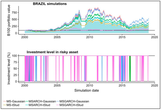
Figure 1.
The historical performance of the six backtested portfolios in the Brazilian stock market.
In order to give support for the results we present, in the last column of Table 7 and in the bottom panel of Figure 1, the investment level in the stock index. As noted in that Table, the average observed investment level (mean risky exposure) in the Brazilian stock index are the third and second lowest levels. The average investment level in the Gaussian MS and MS-GARCH models are 97.36% and 93.75%, respectively. This summary of the investment level in the stock index gives an explanation about the performance improvements achieved with other scenarios. More specifically, the MS-GARCH (the best performing scenario) had significantly lower investment levels in the stock index during the distressing time periods. In addition, the use of Gaussian MS-GARCH models led to a better performance because the forecasted probability of the second regime () leads to more accurate sell decisions during small distress periods. At the end of 2014 and the beginning of 2015, (blue line) an appropriate sell sign is noted, which, during those weeks, allowed the simulated trader to reduce the loss value. In addition, in 2016, the buy decision made in the November 2016 weeks was earlier than the one observed in the other scenarios. Given this, the bottom panel of Figure 1 and the last column of Table 7 give proof about the outperformance of using Gaussian MS-GARCH models.
In a similar fashion to the Brazilian case, we present the results of the simulations in the Chilean market in Table 8. Similarly, for the Brazilian market, the t-Student MS and MS-ARCH models are the worst performers and lead to poorer performance than a passive or a buy-and-hold investment strategy. From all the six simulated portfolios, the one with a Gaussian MS-ARCH model is the one that showed the highest accumulated return (351.4477% or 19.3457% yearly). Furthermore, the improvements in the max drawdown, CVaR, and Sharpe ratio values against the observed ones in Table 6 are of interest.
Table 8.
Performance summary of the Markov-Switching investment strategy applied in the Chilean stock market (from a U.S. dollar-based investor perspective).
In Figure 2, we present the historical performance of the six simulated portfolios of the Chilean market. The over performance in the active trading strategy is observable, especially in the Gaussian MS-ARCH and t-Student MS-GARCH cases. Practically all the MS and MS-GARCH models were very useful to forecast the 2007–2009 distress time period and, in October 2008, practically all were useful to forecast a rebalancing sign. This takes place in order to invest in the risk-free asset during this time period and to avoid the value drawdown that the buy-and-hold strategy had in this time period.
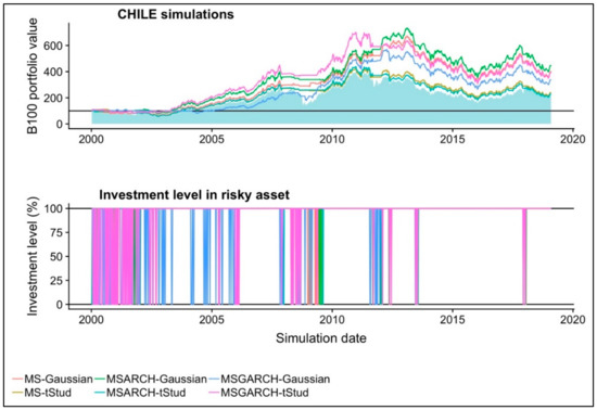
Figure 2.
The historical performance of the six backtested portfolios in the Chilean stock market.
Even if this good performance is held for all the simulated portfolios, the use of Gaussian MS-ARCH models leads to a more sensitive forecast of the distress time period in other time intervals. This last result also led to a better portfolio performance, as noted in the March 2011 period in which this model forecasted the end of the distress time period. This allows the simulated trader to invest in the Chilean stock market during the corresponding upward movement. More specifically, as noted in the bottom panel of Figure 2 for this time period, the use of the Gaussian MS-ARCH model led to an earlier buy decision. This trade enhanced the performance of the simulatedportfolio. Despite this, no other new differences were observed in the six simulated portfolios. This is noted by the fact that the mean investment level in five of the six portfolios (including the best performer) are similar. This led us to conclude that, even if the use of the Gaussian MS-ARCH model leads to more precise investment decisions, this precision is less observable if we compared it with the Brazilian case.
Lastly, we present the performance results of the simulations observed in the Mexican stock market in Table 9. In this last case, the worst performers are the portfolios that used the Gaussian and t-Student MS-ARCH or MS-GARCH models. Only the portfolios with the time-fixed variance generated alpha and, from these two, the Gaussian model is the one with the highest accumulated return (259.3627% or 14.2768% yearly). Furthermore, only these two models (the ones with constant variance) show improvements in the Sharpe ratio when compared with the passive investment strategy.
Table 9.
Performance summary of the Markov-Switching investment strategy applied in the Mexican stock market (from a U.S. dollar-based investor perspective).
This last result can be observed in detail in the historical performance of Figure 3. As noted at the beginning of the simulated period, the two MS portfolios invested in the risk-free asset and they remained invested in it during the 2000 technology stock crisis. Given their less sensitive characteristic to switch the forecast of the smoothed probability of the distress regime, these two portfolios remained invested in the risk-free asset. This is a situation that explains why these two portfolios have a positive performance in the first part of the simulation chart.
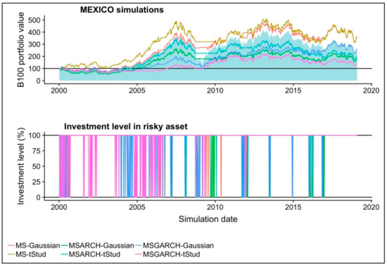
Figure 3.
The historical performance of the six backtested portfolios in the Mexican stock market.
In the 2007–2009 period, these two portfolios invested in the risk-free asset, but the Gaussian pdf MS one remained invested more time in it. This led to a better portfolio value during this period, as noted in the almost flat performance of the Gaussian MS portfolio (gold line).
Lastly, the Gaussian and t-Student MS portfolios had a similar performance in the rest of the simulation, but the Gaussian case led to the more stable performance of both, which suggests that it is preferable to use the Gaussian MS model for active trading in the Mexican stock market.
By following the review of the previous indexes, we found evidence that the better investment timing in the Mexican cases is similar to the Chilean one. That is, the Gaussian MS portfolio is the best performer because, in the previously mentioned 2008 period, the buy trading signal was more accurate. This led to a different performance in the recovering period of 2008–2009. For the specific case of the Mexican index, investing in Gaussian and t-Student MS models led to a more accurate buy signal. This last signal led to a better performance in the 2007–2008 distress time period and to a more accurate buy signal in the March 2001 period. These two accurate buy signals led to better performance and to a higher average investment level in the risky asset or index. As the case of the two previous indexes, the use of MS or MS-GARCH models led to more precise trading signs and to better performance.
In Table 10, we summarize the results of the full time series, recursive test, and the ones of the active investment strategy analysis. As noted for the Brazilian and Chilean markets, the best model to use for risk measurement is the Gaussian with a constant variance MS model because that is the best (lowest BIC) model in most weeks. Despite this result, the Gaussian MS-GARCH and the t-Student MS-ARCH models are the best models (respectively) if the investor wants to perform active investment activities in these markets. Lastly, for the Mexican case, there are no conclusive results between the use of the Gaussian MS or the Gaussian MS-GARCH model for risk measurement purposes. We suggest the Gaussian case, given its marginally higher accumulated return against the t-Student one.
Table 10.
Summary of the full time series as well as recursive and active investment analysis.
Our results are in line with the previous papers in the literature review by showing proofs that it is better to use MS models for active trading in stocks. More specifically, our contributions show that the use of these models and the use of Gaussian MS-GARCH or t-Student MS-ARCH models are preferable in Brazil and Chile. For the Mexican, the use of a Gaussian time-fixed variance MS model is suggested. Therefore, these results give proof that the use of time-varying variance Markov-switching stochastic processes are preferable for the time series characterization of two of these three Latin-American stock indexes. In addition, our results give proof that the use of either MS or MS-GARCH models is useful for active trading decisions in these three stock markets.
5. Conclusions
Markov-Switching (MS) models, as proposed by Hamilton [14,15,16], are very useful to determine if a time series’ stochastic process has several regimes. This allows us to infer an number of location (mean) and scale (standard deviation) parameters. Among the most useful applications of these models in the financial industry, we mention the measurement of the risk level in a given investment with two or more possible regimes or states of nature. For the purposes of this paper, the regime corresponds to a normal or low volatility state of nature at and for a distress or high volatility one. This leads to a very useful risk measure, along with the probability of being in a given regime at or ().
Despite this practical use of the MS models in risk management, little has been written about the use of MS models in stock trading decisions. By knowing the probability of being in a given regime at , an investor can determine whether to invest in a risky (risk-free) asset if the probability of being in a normal (distress) regime is high. This rationale departs from the one proposed by Brooks and Persand [18] and the extensions of Engle, Wahl, and Zagst [21] and De la Torre, Galeana, and Álvarez-García [22]. These previous works test the benefit of investing in a given developed financial market with MS models.
Given the scant literature review of MS models for stock trading, there is no work that test their use in the three most traded Latin American markets from a U.S. dollar-based investor perspective. Additionally, none of the related previous works test the benefit of using a MS model with ARCH (MS-ARCH) or GARCH (MS-GARCH) variances in trading decisions.
Departing from these two issues, the paper tests the use of MS, MS-ARCH, or MS-GARCH models in the Brazilian, Chilean, and Mexican stock markets. With 996 weekly simulations from January 2000 to February 2019 we fitted MS, MS-ARCH, and MS-GARCH models (with Gaussian and t-Student probability density functions) and we ran the next trading rule.
- To invest in the stock market index if the investor expects to be in the low volatility () regime at or
- To invest in the U.S. risk-free asset if the investor expects a high volatility () one.
Our results suggest that the Gaussian MS-GARCH and the t-Student MS-GARCH are the best models for investment decisions in the Brazilian and Chilean stock markets, respectively. For the Mexican case, it is preferable to use a Gaussian MS (with constant variance) model.
Despite the beneficial use of these models for investing in these countries, the conclusions in our results change the risk measurement purposes. This means that, for risk management, it is better to use a Gaussian MS (constant variance) model in the Brazilian and Chilean markets. For the Mexican case, it is preferable to use the Gaussian MS-GARCH model.
Our results could be of theoretical use in order to understand the practical use of MS and MS-GARCH models in forecasting during distressful or highly volatile periods. In addition, this can help us to understand and to prove their application in trading decisions. In practical terms, our results contribute to the literature of using MS and MS-GARCH models in trading. This along with the benefits of their use in the three main Latin-American stock markets from a U.S. dollar-based investor perspective.
As extensions to this paper or research guidelines for further research, we suggest testing the use of other probability functions such as the symmetric and asymmetric Gaussian t-Student or GED regime likelihood functions. This test could be made with homogeneous (the same likelihood function in each regime) or homogeneous probabilities in each regime. As another potential review and extension to our results, we propose the use of MS models with asymmetric GARCH processes (also homogeneous and heterogeneous in each regime) along with fractional integration (long memory modelling).
In addition, the use of MS models with more than two regimes in the stochastic process, along with the test in other stock markets or other type of securities, could be of potential interest. We also believe in theoretical interest for Bayesian Statistics to determine what is best to use: either a rolling time window or a recursive (increasing time series) one. This issue is also of practical interest because the potential use of time rolling windows could enhance the informatic efficiency of the MS-GARCH model estimation method. Despite this, this informatic efficiency could come with a cost in terms of accuracy cost in the estimated parameters. Furthermore, the extension of the current MS trading algorithm with a portfolio of these three indexes (or more) is part of the research agenda suggested. In order to manage a portfolio with several stocks or indexes in a regime-switching context, it is needed to make research efforts in the application of MS correlation models [65,66] in trading algorithms such as ours. Lastly, none of the estimations that we made herein used GARCH models that incorporate the influence of external factors (economic or financials). Models like these ones are studied in Billah, Hyndman, and Koehler [67], Conrad and Loch [68], Amendola et al. [69], and Amendola, Candila, and Gallo [70]. We did not consider this type of MS-GARCH models due to the determination of the proper factors that influence the performance of the three stock indexes. Lastly, given these factors, the determination of the proper MS-GARCH model with these could be another extension for our research efforts.
Author Contributions
Conceptualization, Methodology, Formal Analysis, Investigation, Writing-Original Draft Preparation and Writing-Review & Editing, O.V.D.l.T.-T., E.G.-F., J.Á.-G. All authors have read and agreed to the published version of the manuscript.
Funding
This research received no external funding.
Conflicts of Interest
The authors declare no conflict of interest.
References
- Markowitz, H. Portfolio selection. J. Financ. 1952, 7, 77–91. [Google Scholar] [CrossRef]
- Markowitz, H. Portfolio Selection. Efficient Diversification of Investments; Yale University Press: New Haven, CT, USA, 1959. [Google Scholar]
- Alexander, C. Principal component models for generating large GARCH covariance matrices. Econ. Notes 2002, 31, 337–359. [Google Scholar] [CrossRef]
- Ang, A.; Bekaert, G. International Asset Allocation With Regime Shifts. Rev. Financ. Stud. 2002, 15, 1137–1187. [Google Scholar] [CrossRef]
- Sharpe, W. A simplified model for portfolio analysis. Manag. Sci. 1963, 9, 277–293. [Google Scholar] [CrossRef]
- Sharpe, W. Capital asset prices: A theory of market equilibrium under conditions of risk. J. Financ. 1964, XIX, 425–442. [Google Scholar]
- Engle, R. Autoregressive Conditional Heteroscedasticity with estimates of the variance of United Kingdom inflation. Econometrica 1982, 50, 987–1007. [Google Scholar] [CrossRef]
- Bollerslev, T. A Conditionally Heteroskedastic time series model for speculative prices and rates of return. Rev. Econ. Stat. 1987, 69, 542–547. [Google Scholar] [CrossRef]
- Dueker, M. Markov Switching in GARCH Processes and Mean- Reverting Stock-Market Volatility. J. Bus. Econ. Stat. 1997, 15, 26–34. [Google Scholar]
- Lamoureux, C.G.; Lastrapes, W.D. Persistence in Variance, Structural Change, and the GARCH Model. J. Bus. Econ. Stat. 1990, 8, 225–234. [Google Scholar] [CrossRef]
- Canarella, G.; Pollard, S.K. A switching ARCH (SWARCH) model of stock market volatility: Some evidence from Latin America. Int. Rev. Econ. 2007, 54, 445–462. [Google Scholar] [CrossRef]
- Klaassen, F. Improving GARCH volatility forecasts with regime-switching GARCH. In Advances in Markov-Switching Models; Physica-Verlag HD: Heidelberg, Germany, 2002; pp. 223–254. [Google Scholar]
- Haas, M.; Mittnik, S.; Paolella, M.S. A New Approach to Markov-Switching GARCH Models. J. Financ. Econom. 2004, 2, 493–530. [Google Scholar] [CrossRef]
- Hamilton, J.D. A New Approach to the Economic Analysis of Nonstationary Time Series and the Business Cycle. Econometrica 1989, 57, 357–384. [Google Scholar] [CrossRef]
- Hamilton, J.D. Analysis of time series subject to changes in regime. J. Econom. 1990, 45, 39–70. [Google Scholar] [CrossRef]
- Hamilton, J.D. Time Series Analysis; Princeton University Press: Princeton, NJ, USA, 1994. [Google Scholar]
- Hamilton, D.; Susmel, R. Autorregresive conditional heteroskedasticity and changes in regime. J. Econom. 1994, 64, 307–333. [Google Scholar] [CrossRef]
- Brooks, C.; Persand, G. The trading profitability of forecasts of the gilt–equity yield ratio. Int. J. Forecast. 2001, 17, 11–29. [Google Scholar] [CrossRef]
- Kritzman, M.; Page, S.; Turkington, D. Regime Shifts: Implications for Dynamic Strategies. Financ. Anal. J. 2012, 68, 22–39. [Google Scholar] [CrossRef]
- Hauptmann, J.; Hoppenkamps, A.; Min, A.; Ramsauer, F.; Zagst, R. Forecasting market turbulence using regime-switching models. Financ. Mark. Portf. Manag. 2014, 28, 139–164. [Google Scholar] [CrossRef]
- Engel, J.; Wahl, M.; Zagst, R. Forecasting turbulence in the Asian and European stock market using regime-switching models. Quant. Financ. Econ. 2018, 2, 388–406. [Google Scholar] [CrossRef]
- De la Torre, O.; Galeana-Figueroa, E.; Álvarez-García, J. Using Markov-Switching models in Italian, British, U.S. and Mexican equity portfolios: A performance test. Electron. J. Appl. Stat. Anal. 2018, 11, 489–505. [Google Scholar] [CrossRef]
- World Federation of Exchanges Statistics—The World Federation of Exchanges. Available online: https://www.world-exchanges.org/our-work/statistics (accessed on 15 February 2019).
- MSCI Inc. MSCI Global Investable Market Indexes Methodology. Available online: http://www.msci.com/eqb/methodology/meth_docs/MSCI_Jan2015_GIMIMethodology_vf.pdf (accessed on 2 May 2018).
- Ang, A.; Bekaert, G. Regime Switches in Interest Rates. J. Bus. Econ. Stat. 2002, 20, 163–182. [Google Scholar] [CrossRef]
- Ang, A.; Bekaert, G. Short rate nonlinearities and regime switches. J. Econ. Dyn. Control 2002, 26, 1243–1274. [Google Scholar] [CrossRef]
- Klein, A.C. Time-variations in herding behavior: Evidence from a Markov switching SUR model. J. Int. Financ. Mark. Inst. Money 2013, 26, 291–304. [Google Scholar] [CrossRef]
- Areal, N.; Cortez, M.C.; Silva, F. The conditional performance of US mutual funds over different market regimes: Do different types of ethical screens matter? Financ. Mark. Portf. Manag. 2013, 27, 397–429. [Google Scholar] [CrossRef]
- Zheng, T.; Zuo, H. Reexamining the time-varying volatility spillover effects: A Markov switching causality approach. N. Am. J. Econ. Financ. 2013, 26, 643–662. [Google Scholar] [CrossRef]
- Alexander, C.; Kaeck, A. Regime dependent determinants of credit default swap spreads. J. Bank. Financ. 2007, 1008–1021. [Google Scholar] [CrossRef]
- Castellano, R.; Scaccia, L. Can CDS indexes signal future turmoils in the stock market? A Markov switching perspective. CEJOR 2014, 22, 285–305. [Google Scholar] [CrossRef]
- Ma, J.; Deng, X.; Ho, K.-C.; Tsai, S.-B. Regime-Switching Determinants for Spreads of Emerging Markets Sovereign Credit Default Swaps. Sustainability 2018, 10, 1–17. [Google Scholar] [CrossRef]
- Piger, J.; Max, J.; Chauvet, M. Smoothed U.S. Recession Probabilities [RECPROUSM156N]. Available online: https://fred.stlouisfed.org/series/RECPROUSM156N (accessed on 22 October 2019).
- Chauvet, M. An econometric characterization of business cycle dynamics with factor structure and regime switching. Int. Econ. Rev. 2000, 10, 127–142. [Google Scholar] [CrossRef]
- Sottile, P. On the political determinants of sovereign risk: Evidence from a Markov-switching vector autoregressive model for Argentina. Emerg. Mark. Rev. 2013, 160–185. [Google Scholar] [CrossRef]
- Riedel, C.; Thuraisamy, K.S.; Wagner, N. Credit cycle dependent spread determinants in emerging sovereign debt markets. Emerg. Mark. Rev. 2013, 17, 209–223. [Google Scholar] [CrossRef]
- Zhao, H. Dynamic relationship between exchange rate and stock price: Evidence from China. Res. Int. Bus. Financ. 2010, 24, 103–112. [Google Scholar] [CrossRef]
- Walid, C.; Chaker, A.; Masood, O.; Fry, J. Stock market volatility and exchange rates in emerging countries: A Markov-state switching approach. Emerg. Mark. Rev. 2011, 12, 272–292. [Google Scholar] [CrossRef]
- Walid, C.; Duc Khuong, D. Exchange rate movements and stock market returns in a regime-switching environment: Evidence for BRICS countries. Res. Int. Bus. Financ. 2014, 46–56. [Google Scholar] [CrossRef]
- Rotta, P.N.; Valls Pereira, P.L. Analysis of contagion from the dynamic conditional correlation model with Markov Regime switching. Appl. Econ. 2016, 48, 2367–2382. [Google Scholar] [CrossRef]
- Mouratidis, K.; Kenourgios, D.; Samitas, A.; Vougas, D. Evaluating currency crises: A multivariate markov regime switching approach. Manchester Sch. 2013, 81, 33–57. [Google Scholar] [CrossRef]
- Miles, W.; Vijverberg, C.-P. Formal targets, central bank independence and inflation dynamics in the UK: A Markov-Switching approach. J. Macroecon. 2011, 33, 644–655. [Google Scholar] [CrossRef]
- Lopes, J.M.; Nunes, L.C. A Markov regime switching model of crises and contagion: The case of the Iberian countries in the EMS. J. Macroecon. 2012, 34, 1141–1153. [Google Scholar] [CrossRef]
- Kanas, A. Regime linkages between the Mexican currency market and emerging equity markets. Econ. Model. 2005, 22, 109–125. [Google Scholar] [CrossRef]
- Alvarez-Plata, P.; Schrooten, M. The Argentinean currency crisis: A Markov-switching model estimation. Dev. Econ. 2006, 44, 79–91. [Google Scholar] [CrossRef]
- Parikakis, G.S.; Merika, A. Evaluating volatility dynamics and the forecasting ability of Markov switching models. J. Forecast. 2009, 28, 736–744. [Google Scholar] [CrossRef]
- Girdzijauskas, S.; Štreimikienė, D.; Čepinskis, J.; Moskaliova, V.; Jurkonytė, E.; Mackevičius, R. Formation of Economic bubles: Cuases and possible interventions. Technol. Econ. Dev. Econ. 2009, 15, 267–280. [Google Scholar] [CrossRef]
- Dubinskas, P.; Stungurienė, S. Alterations in the financial markets of the baltic countries and Russia in the period of Economic cownturn. Technol. Econ. Dev. Econ. 2010, 16, 502–515. [Google Scholar] [CrossRef]
- Kutty, G. The Relationship Between Exchange Rates and Stock Prices: The Case of Mexico. N. Am. J. Financ. Bank. Res. 2010, 4, 1–12. [Google Scholar]
- Ahmed, R.R.; Vveinhardt, J.; Štreimikiene, D.; Ghauri, S.P.; Ashraf, M. Stock returns, volatility and mean reversion in Emerging and Developed financial markets. Technol. Econ. Dev. Econ. 2018, 24, 1149–1177. [Google Scholar] [CrossRef]
- Dufrénot, G.; Mignon, V.; Péguin-Feissolle, A. The effects of the subprime crisis on the Latin American financial markets: An empirical assessment. Econ. Model. 2011, 28, 2342–2357. [Google Scholar] [CrossRef]
- Sosa, M.; Ortiz, E.; Cabello, A. Dynamic Linkages between Stock Market and Exchange Rate in mila Countries: A Markov Regime Switching Approach (2003-2016). Análisis Económico 2018, 33, 57–74. [Google Scholar] [CrossRef]
- Cabrera, G.; Coronado, S.; Rojas, O.; Venegas-Martínez, F. Synchronization and Changes in Volatilities in the Latin American’S Stock Exchange Markets. Int. J. Pure Appl. Math. 2017, 114. [Google Scholar] [CrossRef]
- De la Torre, O.; Álvarez-García, J.; Galeana-Figueroa, E. A Comparative Performance Review of the Venezuelan, Latin-American and Emerging Markets Stock Indexes with the North-American Ones Using a Gaussian Two-Regime Markov-Switching Model. Espacios 2018, 39, 1–10. [Google Scholar]
- Baum, L.E.; Petrie, T.; Soules, G.; Weiss, N. A maximizaiton thecnique occurring in the Statistical analysis of probabilistic functions of Markov chains. Ann. Appl. Stat. 1970, 41, 164–171. [Google Scholar]
- Viterbi, A. Error bounds for convolutional codes and an asymptotically optimum decoding algorithm. IEEE Trans. Inf. Theory 1967, 13, 260–269. [Google Scholar] [CrossRef]
- Ardia, D.; Bluteau, K.; Boudt, K.; Trottier, D. Markov–Switching GARCH Models in R: The MSGARCH Package. J. Stat. Softw. 2019, 91, 38. [Google Scholar] [CrossRef]
- Kim, C.-J. Dynamic linear models with Markov-switching. J. Econom. 1994, 60, 1–22. [Google Scholar] [CrossRef]
- MSCI Inc. End of Day Index Data Search—MSCI. Available online: https://www.msci.com/end-of-day-data-search (accessed on 2 April 2019).
- Refinitiv Refinitiv Eikon. Available online: https://eikon.thomsonreuters.com/index.html (accessed on 3 June 2019).
- Akaike, H. A new look at the statistical model identification. IEEE Trans. Automat. Contr. 1974, 19, 716–723. [Google Scholar] [CrossRef]
- Schwarz, G. Estimating the dimension of a model. Ann. Stat. 1978, 6, 461–464. [Google Scholar] [CrossRef]
- Hannan, E.J.; Quinn, B.G. The Determination of the Order of an Autoregression. J. R. Stat. Soc. Ser. B 1979, 41, 190–195. [Google Scholar] [CrossRef]
- Artzner, P.; Delbaen, F.; Eber, J.M.; Heath, D. Coherent measures of risk. Math. Financ. 1999, 9, 203–228. [Google Scholar] [CrossRef]
- Pelletier, D. Regime Switching for Dynamic Correlations. J. Econometrics 2006, 131, 445–473. [Google Scholar] [CrossRef]
- Haas, M. Covariance forecasts and long-run correlations in a Markov-switching model for dynamic correlations. Financ. Res. Lett. 2010, 7, 86–97. [Google Scholar] [CrossRef]
- Billah, B.; Hyndman, R.J.; Koehler, A.B. Empirical information criteria for time series forecasting model selection. J. Stat. Comput. Simul. 2005, 75, 831–840. [Google Scholar] [CrossRef]
- Conrad, C.; Loch, K. Journal of Applied Econometrics. J. Appl. Econom. 2015, 30, 1090–1114. [Google Scholar] [CrossRef]
- Amendola, A.; Candila, V.; Scognamillo, A. On the influence of US monetary policy on crude oil price volatility more, the out-of-sample forecasting procedure shows that including these additional macroeconomic variables generally improves the forecasting performance. Empir. Econ. 2017, 52, 155–178. [Google Scholar] [CrossRef]
- Amendola, A.; Candila, V.; Gallo, G.M. On the asymmetric impact of macro-variables on volatility. Econ. Model. 2019, 76, 135–152. [Google Scholar] [CrossRef]
© 2020 by the authors. Licensee MDPI, Basel, Switzerland. This article is an open access article distributed under the terms and conditions of the Creative Commons Attribution (CC BY) license (http://creativecommons.org/licenses/by/4.0/).