Effects of Uncertainty Shocks on Household Consumption and Working Hours: A Fuzzy Cognitive Map-Based Approach


Abstract
1. Introduction
2. Literature Review
3. Fuzzy Cognitive Map
- Step 1. Determine the weights and fuzzify input concept values.
- Step 2. Determine the inference rule and transformation function to be used in FCM inference.
- Step 3. Convert the output concept values into real data values for further analysis.
4. Data Analysis
4.1. Data Description
4.2. FCM Setting and Inference Scheme
| Algorithm 1: Forecasting Household Consumption and Weekly Working Hours with FCM |
 |
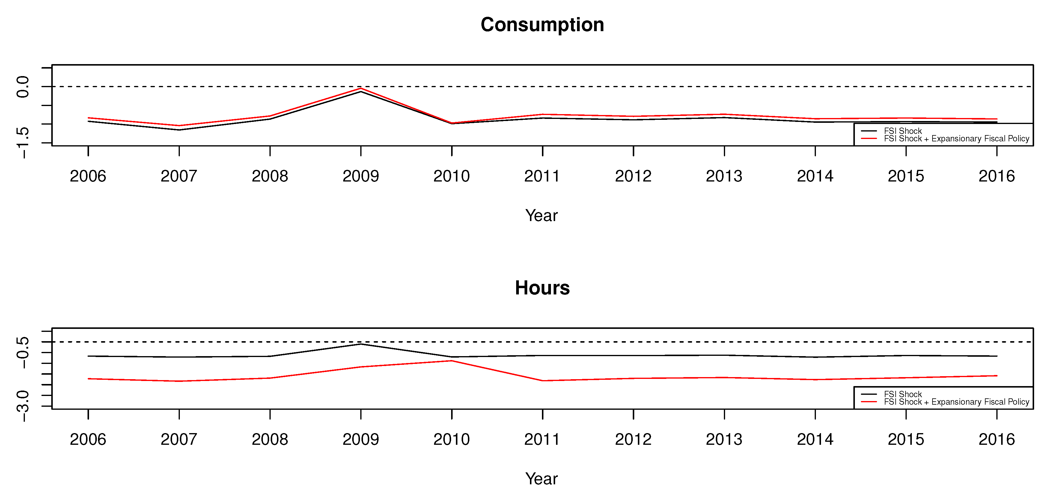
5. Scenario Analysis
5.1. Effects of FSI Shock
5.2. Effects of EPU Shock
6. Conclusions
Author Contributions
Funding
Acknowledgments
Conflicts of Interest
Abbreviations
| FCM | Fuzzy Cognitive Map |
| FSI | Financial Stress Index |
| EPU | Economic Policy Uncertainty |
| VAR | Vector Autoregression |
| DSGE | Dynamic Stochastic General Equilibrium |
References
- Carvalho, J.P. On the semantics and the use of fuzzy cognitive maps and dynamic cognitive maps in social sciences. Fuzzy Sets Syst. 2013, 124, 6–19. [Google Scholar] [CrossRef]
- Sanchez-Roger, M.; Oliver-Alfonso, M.D.; Sanchis-Pedregosa, C. Fuzzy logic and its uses in finance: A systematic review exploring its potential to deal with banking crises. Mathematics 2019, 7, 1091. [Google Scholar] [CrossRef]
- Ludvigson, S.C.; Ma, S.; Ng, S. Uncertainty and business cycles: Exogenous impulse or endogenous response? Am. Econ. J. Macroecon. 2020. forthcoming. [Google Scholar]
- Choi, S.; Shim, M. Financial vs. policy uncertainty in emerging market economies. Open Econ. Rev. 2019, 30, 297–318. [Google Scholar] [CrossRef]
- Stockhammar, P.; Österholm, P. The impact of US uncertainty shocks on small open economies. Open Econ. Rev. 2017, 28, 347–368. [Google Scholar] [CrossRef]
- Mumtaz, H.; Theodoridis, K. The changing transmission of uncertainty shocks in the U.S. J. Bus. Econ. Stat. 2018, 36, 239–252. [Google Scholar] [CrossRef]
- Bloom, N. The impact of uncertainty shocks. Econometrica 2009, 77, 623–685. [Google Scholar]
- Christiano, L.J.; Motto, R.M.; Rostagno, M. Risk shocks. Am. Econ. Rev. 2014, 104, 27–65. [Google Scholar] [CrossRef]
- Baker, S.R.; Bloom, N.; Davis, S.J. Measuring economic policy uncertainty. Q. J. Econ. 2016, 131, 1593–1636. [Google Scholar] [CrossRef]
- Fernández-Villaverde, J.; Guerrón-Quintana, P.; Kuester, K.; Rubio-Ramírez, J. Fiscal volatility shocks and economic activity. Am. Econ. Rev. 2015, 105, 3352–3384. [Google Scholar] [CrossRef]
- Carroll, C.D. Buffer-stock saving and the life cycle/permanent income hypothesis. Q. J. Econ. 1997, 112, 1–55. [Google Scholar] [CrossRef]
- Carroll, C.D.; Hall, R.E.; Zeldes, S.P. The buffer-stock theory of saving: Some macroeconomic evidence. Brookings Pap. Econ. Act. 1992, 1992, 61–156. [Google Scholar] [CrossRef]
- Deaton, A. Saving and liquidity constraints. Econometrica 1991, 59, 1221–1248. [Google Scholar] [CrossRef]
- Flodén, M. Labour supply and saving under uncertainty. Econ. J. 2006, 116, 721–737. [Google Scholar] [CrossRef]
- Pijoan-Mas, J. Precautionary savings or working longer hours? Rev. Econ. Dyn. 2006, 9, 326–352. [Google Scholar] [CrossRef]
- Nocetti, D.; Smith, W.T. Precautionary saving and endogenous labor supply with and without intertemporal expected utility. J. Money Credit Bank. 2011, 43, 1475–1504. [Google Scholar] [CrossRef]
- Wu, C.; Krueger, D. Consumption insurance against wage risk: Family labor supply and optimal progressive income taxation. Am. Econ. J. Macroecon. 2020. forthcoming. [Google Scholar]
- Kosko, B. Fuzzy cognitive maps. Int. J. Man-Mach. Stud. 1986, 24, 65–75. [Google Scholar] [CrossRef]
- Papageorgiou, E.I. Methods and algorithms for fuzzy cognitive map-based modeling. In Fuzzy Cognitive Maps for Applied Sciences and Engineering; Papageorgiou, E.I., Ed.; Springer: Berlin, Germany, 2014; pp. 1–28. [Google Scholar]
- Boutalis, Y.; Kottas, T.L.; Christodoulou, M. Adaptive estimation of fuzzy cognitive maps with proven stability and parameter convergence. IEEE Trans. Fuzzy Syst. 2009, 17, 874–889. [Google Scholar] [CrossRef]
- Bhattarai, S.; Chatterjee, A.; Park, W.Y. Global spillover effects of US uncertainty. J. Monet. Econ. 2019. forthcoming. [Google Scholar] [CrossRef]
- Cardarelli, R.; Elekdag, S.; Lall, S. Financial stress and economic contractions. J. Financ. Stab. 2011, 7, 78–97. [Google Scholar] [CrossRef]
- Yoon, J.H. Fuzzy mediation analysis. Int. J. Fuzzy Syst. 2020, 22, 338–349. [Google Scholar] [CrossRef]
- Papageorgiou, E.I.; Stylios, C.; Groumpos, P. Fuzzy cognitive map learning based on nonlinear Hebbian rule. In AI 2003: Advances in Artificial Intelligence; Gedeon, T.D., Fung, L.C.C., Eds.; Springer: Berlin, Germany, 2003; pp. 256–268. [Google Scholar]
- Gupta, S.; Gupta, S. Modeling economic system using fuzzy cognitive maps. Int. J. Syst. Assur. Eng. Manag. 2017, 8, 1472–1486. [Google Scholar] [CrossRef]
- Basu, S.; Bundick, B. Uncertainty shocks in a model of effective demand. Econometrica 2017, 85, 937–958. [Google Scholar] [CrossRef]


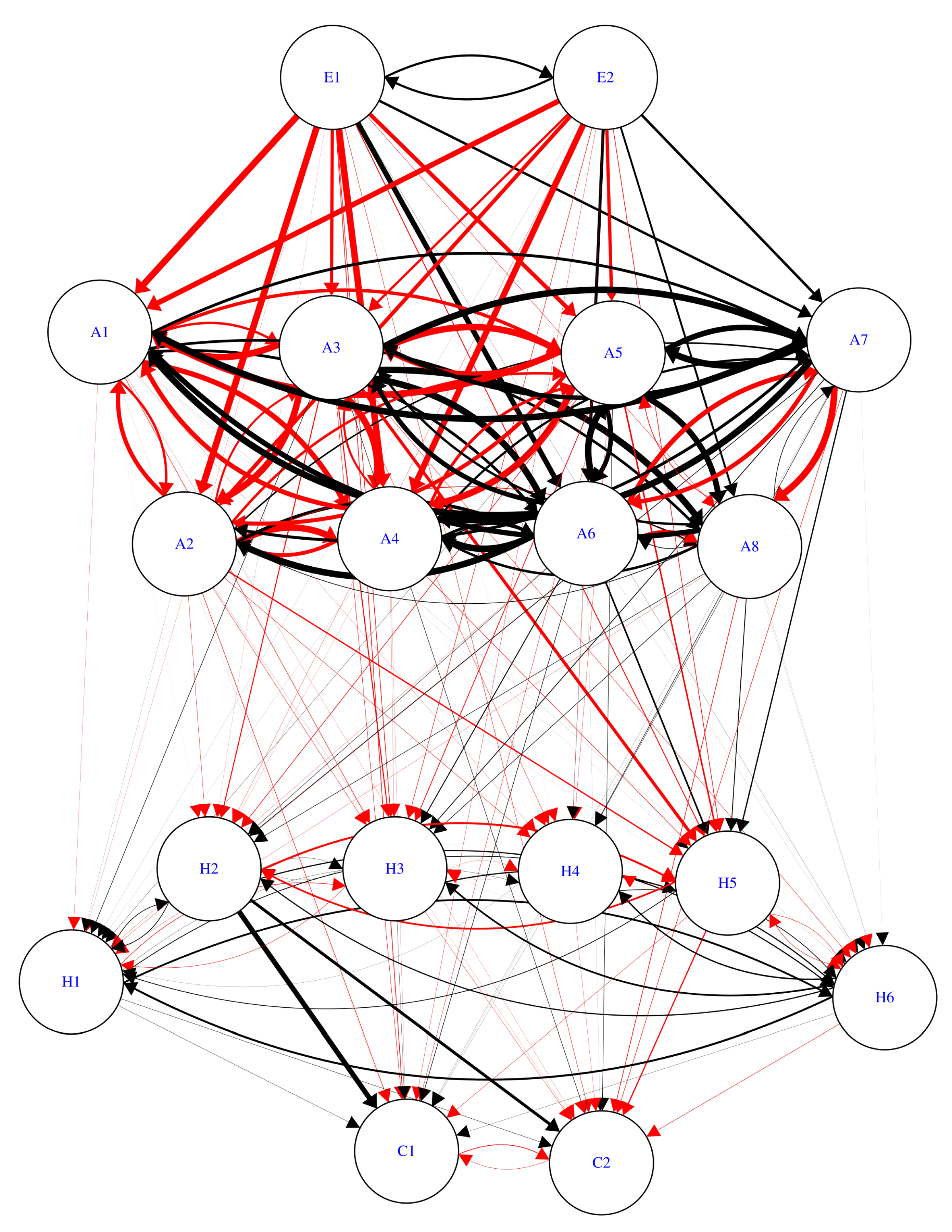
| Label | Concept | Label | Concept |
|---|---|---|---|
| E1 | Financial Stress Index | H1 | Debt |
| E2 | Economic Policy Uncertainty | H2 | Financial Income |
| A1 | Consumer Sentiment Index | H3 | Labor Income |
| A2 | Bank Lending Attitude Index | H4 | Real Estate Income |
| A3 | Household Lending Interest Rate | H5 | Transfer Income |
| A4 | KOSPI | H6 | Asset |
| A5 | Unemployment Rate | C1 | Consumption |
| A6 | Inflation Rate | C2 | Working Hours |
| A7 | GDP Growth Rate | ||
| A8 | Government Expenditure |
| E1 | E2 | A1 | A2 | A3 | A4 | A5 | A6 | A7 | |
|---|---|---|---|---|---|---|---|---|---|
| E1 | 0 | 0.336 | −1 | −1 | −0.488 | −1 | −0.623 | 0.796 | 0.374 |
| E2 | 0.336 | 0 | −0.815 | −0.591 | −0.352 | −0.920 | −0.498 | 0.463 | 0.393 |
| A1 | 0 | 0 | 0 | −0.368 | −0.364 | −0.800 | −0.523 | 0.430 | 0.435 |
| A2 | 0 | 0 | −0.649 | 0 | −0.304 | −1 | −0.387 | 0.526 | 0.229 |
| A3 | 0 | 0 | −1 | −1 | 0 | −1 | −1 | 1 | 1 |
| A4 | 0 | 0 | −0.714 | −0.580 | −0.313 | 0 | −0.449 | 0.428 | 0.343 |
| A5 | 0 | 0 | −1 | −0.615 | −0.643 | −1 | 0 | 0.707 | 0.852 |
| A6 | 0 | 0 | 1 | 1 | 0.730 | 1 | 0.988 | 0 | −0.738 |
| A7 | 0 | 0 | 1 | 0.459 | 0.674 | 1 | 1 | −0.663 | 0 |
| A8 | 0 | 0 | 0.808 | 0.100 | 0.359 | 0.381 | −0.100 | 0.100 | 0.100 |
| H1 | 0 | 0 | 0 | 0 | 0 | 0 | 0 | 0 | 0 |
| H2 | 0 | 0 | 0 | 0 | 0 | 0 | 0 | 0 | 0 |
| H3 | 0 | 0 | 0 | 0 | 0 | 0 | 0 | 0 | 0 |
| H4 | 0 | 0 | 0 | 0 | 0 | 0 | 0 | 0 | 0 |
| H5 | 0 | 0 | 0 | 0 | 0 | 0 | 0 | 0 | 0 |
| H6 | 0 | 0 | 0 | 0 | 0 | 0 | 0 | 0 | 0 |
| C1 | 0 | 0 | 0 | 0 | 0 | 0 | 0 | 0 | 0 |
| C2 | 0 | 0 | 0 | 0 | 0 | 0 | 0 | 0 | 0 |
| A8 | H1 | H2 | H3 | H4 | H5 | H6 | C1 | C2 | |
| E1 | −0.055 | −0.020 | −0.015 | −0.090 | −0.006 | −0.134 | 0.023 | −0.098 | −0.058 |
| E2 | 0.288 | 0.011 | −0.034 | −0.071 | −0.031 | −0.091 | 0.011 | −0.039 | 0 |
| A1 | 0.409 | −0.023 | −0.003 | −0.071 | −0.023 | 0.007 | 0.011 | −0.010 | −0.023 |
| A2 | −0.115 | 0.014 | −0.046 | −0.053 | −0.058 | −0.196 | −0.008 | −0.073 | −0.018 |
| A3 | 1 | 0.079 | −0.149 | −0.153 | −0.050 | −0.479 | −0.055 | −0.060 | 0.069 |
| A4 | 0.172 | 0.010 | −0.019 | −0.024 | −0.004 | −0.073 | 0.002 | −0.021 | −0.005 |
| A5 | 0.894 | 0.034 | −0.091 | −0.113 | −0.037 | −0.226 | 0.002 | −0.050 | 0.066 |
| A6 | −0.465 | −0.028 | 0.061 | 0.140 | 0.018 | 0.251 | −0.012 | 0.080 | 0.009 |
| A7 | −1 | −0.034 | 0.095 | 0.115 | 0.072 | 0.191 | 0.005 | 0.018 | −0.072 |
| A8 | 0 | −0.032 | 0.074 | 0.084 | 0.051 | 0.125 | −0.012 | 0.010 | −0.092 |
| H1 | 0 | 0 | 0.099 | −0.079 | 0.030 | 0.116 | 0.280 | 0.041 | 0.050 |
| H2 | 0 | 0.108 | 0 | 0.036 | −0.005 | −0.299 | 0.174 | 0.779 | 0.452 |
| H3 | 0 | −0.058 | 0.024 | 0 | −0.021 | −0.008 | 0.177 | 0.031 | −0.042 |
| H4 | 0 | 0.017 | −0.002 | −0.016 | 0 | −0.007 | 0.107 | 0.019 | −0.030 |
| H5 | 0 | 0.112 | −0.266 | −0.010 | −0.0119 | 0 | −0.057 | −0.051 | −0.180 |
| H6 | 0 | 0.305 | 0.173 | 0.260 | 0.210 | −0.064 | 0 | 0.030 | −0.063 |
| C1 | 0 | 0 | 0 | 0 | 0 | 0 | 0 | 0 | −0.101 |
| C2 | 0 | 0 | 0 | 0 | 0 | 0 | 0 | −0.048 | 0 |
| No Expansionary Policy | Expansionary Policy | |
|---|---|---|
| C1 | −0.8591 | −0.7728 |
| (0.2451) | (0.2469) | |
| C2 | −0.6149 | −1.5915 |
| (0.1655) | (0.2821) | |
| H1 | −0.7339 | −1.7984 |
| (0.2637) | (0.5070) | |
| H2 | −0.0369 | 0.0000 |
| (0.0117) | (0.0182) | |
| H3 | −0.2337 | 0.9146 |
| (0.0640) | (0.3195) | |
| H4 | −0.0122 | 0.1108 |
| (0.0093) | (0.0760) | |
| H5 | −0.0830 | −0.0032 |
| (0.0348) | (0.0380) | |
| H6 | 0.9234 | 0.4678 |
| (0.3003) | (0.2897) |
| No Expansionary Policy | Expansionary Policy | |
|---|---|---|
| C1 | −0.8577 | −0.7715 |
| (0.8807) | (0.8824) | |
| C2 | −0.6144 | −1.5901 |
| (0.6163) | (0.6403) | |
| H1 | −0.7482 | −1.8111 |
| (0.7970) | (0.8871) | |
| H2 | −0.0306 | 0.0066 |
| (0.0374) | (0.0542) | |
| H3 | −0.2253 | 0.9232 |
| (0.2313) | (0.4279) | |
| H4 | −0.0110 | 0.1133 |
| (0.0125) | (0.0798) | |
| H5 | −0.0651 | 0.0132 |
| (0.0929) | (0.1164) | |
| H6 | 0.8641 | 0.4094 |
| (0.9480) | (0.9955) |
© 2020 by the authors. Licensee MDPI, Basel, Switzerland. This article is an open access article distributed under the terms and conditions of the Creative Commons Attribution (CC BY) license (http://creativecommons.org/licenses/by/4.0/).
Share and Cite
Yun, Y.; Jung, H.-Y. Effects of Uncertainty Shocks on Household Consumption and Working Hours: A Fuzzy Cognitive Map-Based Approach. Mathematics 2020, 8, 889. https://doi.org/10.3390/math8060889
Yun Y, Jung H-Y. Effects of Uncertainty Shocks on Household Consumption and Working Hours: A Fuzzy Cognitive Map-Based Approach. Mathematics. 2020; 8(6):889. https://doi.org/10.3390/math8060889
Chicago/Turabian StyleYun, Yeonggyu, and Hye-Young Jung. 2020. "Effects of Uncertainty Shocks on Household Consumption and Working Hours: A Fuzzy Cognitive Map-Based Approach" Mathematics 8, no. 6: 889. https://doi.org/10.3390/math8060889
APA StyleYun, Y., & Jung, H.-Y. (2020). Effects of Uncertainty Shocks on Household Consumption and Working Hours: A Fuzzy Cognitive Map-Based Approach. Mathematics, 8(6), 889. https://doi.org/10.3390/math8060889