Stable Finite-Difference Methods for Elastic Wave Modeling with Characteristic Boundary Conditions

Abstract

In this paper, a new stable finite-difference (FD) method for solving elastodynamic equations is presented and applied on the Biot and Biot/squirt (BISQ) models. This method is based on the operator splitting theory and makes use of the characteristic boundary conditions to confirm the overall stability which is demonstrated with the energy method. Through the stability analysis, it is showed that the stability conditions are more generous than that of the traditional algorithms. It allows us to use the larger time step $\tau$ in the procedures for the elastic wave field solutions. This context also provides and compares the computational results from the stable Biot and unstable BISQ models. The comparisons show that this FD method can apply a new numerical technique to detect the stability of the seismic wave propagation theories. The rigorous theoretical stability analysis with the energy method is presented and the stable/unstable performance with the numerical solutions is also revealed. The truncation errors and the detailed stability conditions of the FD methods with different characteristic boundary conditions have also been evaluated. Several applications of the constructed FD methods are presented. When the stable FD methods to the elastic wave models are applied, an initial stability test can be established. Further work is still necessary to improve the accuracy of the method.

1. Introduction

The propagation dynamics of seismic waves in fluid saturated porous media are of great importance for reservoir rock characterization and attract many geoscientists. The elastic waves travel through the underground material with attenuation and dispersion which is closely related to the heterogeneities of the porous continuum properties [1,2]. Attenuation is the exponential decay of the wave amplitude with distance and dispersion means the variation of wave velocity with frequency. It is commonly accepted that the wave propagation phenomenon can be described by the partial differential equations as functions of time t and space position x [1,3]. Various theories [4,5,6,7,8] focus on the dissipation mechanism of wave energy. Among the various theories, the Biot and squirt-flow mechanisms are believed to be the most important ones [6,9]. They have served as the rigorous and formal foundations to study acoustic wave propagation in saturated porous media. Numerous efforts are made to discuss the different form and numerical implementation of these two mechanisms [10]. Based on these theories, recently much attention has been paid in the literature on investigating the seismic wave propagation theories by various numerical methods, such as finite-difference (FD) and finite-element (FE) methods. When considering the simulation of wave propagation in saturated media, FD methods are well received and applied with success to numerous physical problems [11].

On the elastic wave numerical simulation or reverse-time migration, the FD method with a suitable grid is widely applied, such as the staggered grid and the rotated staggered grid. In the first-order velocity-stress hyperbolic system, the FD staggered-grid method applied with the Yee scheme is popular, but the stability of the numerical solution has been shown only in some cases [12]. Virieux provides the stability condition of the 2-order difference scheme based on a staggered grid [13]. However, when applying the FD staggered grid method on the anisotropic media, it is found that the global error significantly increases [14]. For this, Saenger et al. [15] proposed the FD rotated staggered grid method by which the accuracy is increased. Subsequently, it was discovered that this method is unstable on the boundary [16].

The construction of the algorithm usually focuses only on the accuracy. However, the stability condition is also a key factor during the elastic wave numerical simulation. The condition remands that the time step length of discrete differential should be small enough to ensure that the computation in stable. Thus far, extensive efforts have been made to overcome the limitations in calculations. Even though these conventional methods have offered great success in many applications, there can be some uncertainties and extra discrepancies owing to the lack of stable difference method and suitable boundary conditions. Thus, a stable and accurate FD method is needed to address such problems. In addition, geophysicists normally use the Fourier method to discuss the stability of the difference scheme and get some criteria, such as Von Neumann conditions [17]. This method is simple but limited to the linear differential equations with constant coefficients. For this, an energy method that can be directly applied to the nonlinear systems is considered in this work.

Some interesting combinations of difference scheme and boundary condition might overcome these limits. The idea is to use the difference scheme on the basis of the time-splitting method and to consider the adjusted characteristic boundary conditions to assure the overall stability and accuracy of the system, which is shown in Section 2. Its validity, accuracy, and applicability are systematically and theoretically investigated in Section 3. We also test the new stable finite-difference methods by applying it to the stable Biot model and unstable BISQ model with some experimental data-parameters from the paper by Yang et al. [18]. All numerical results encountered in Section 4 show that the finite difference methods and characteristic boundary conditions are suitable to simulate the wave propagation in a long time period. Therefore, for the stability analysis of different wave propagation models, the schemes are appropriate choices.

2. Related Work

This section presents the governing equations and the related solutions of the elastic wave modeling. The one-dimensional medium of the Biot/squirt (BISQ) elastic-wave equations can be represented as [6]:

$$\begin{array}{cc}\hfill & v_t=R{\rho }_{22}{\tau }_x+R{\rho }_2\varphi P_x+R{\rho }_2\frac{\eta {\varphi }^2}{\kappa }(w-v),\hfill \\ \hfill & w_t=-R{\rho }_{12}{\tau }_x-R{\rho }_1\varphi P_x-R{\rho }_1\frac{\eta {\varphi }^2}{\kappa }(w-v),\hfill \\ \hfill & {\tau }_t=\left[M+\frac{\alpha FS(\alpha -\varphi )}{\varphi }\right]v_x+\alpha FS{w}_x,\hfill \\ \hfill & P_t=-FS\frac{\alpha -\varphi }{\varphi }{v}_x-FS{w}_x.\hfill \end{array}$$

(1)

Here, $v=v(x,t)$ and $w=w(x,t)$ are the respective solid’s and fluid’s velocities at the position-time point $(x,t)\in R\times [0,T]$, $\tau$ is the total stress of the bulk material, $P=P(x,t)$ is the total fluid pressure; $\varphi \in (0,1)$ is the porosity of the solid, M is the uniaxial modulus of the skeleton in drained conditions, $\alpha$ is the poroelastic coefficient, $\eta$ is the viscosity of the fluid, $\kappa$ is the permeability of the skeleton, F and S are the Biot-flow and characteristic squirt-flow coefficients, $R={({\rho }_1{\rho }_{22}-{\rho }_2{\rho }_{12})}^{-1}$, and

$${\rho }_{22}=\varphi {\rho }_f-{\rho }_{12},{\rho }_{12}=-{\rho }_a,{\rho }_1=(1-\varphi ){\rho }_s,{\rho }_2=\varphi {\rho }_f,$$

${\rho }_s$, ${\rho }_f$, and ${\rho }_a$ are the respective solid’s, fluid’s, and additional coupling densities. Subscripts x and t indicate partial derivatives (e.g., $P_x=\frac{\partial P}{\partial x}$, $u_{tt}=\frac{{\partial }^{2}u}{\partial t^2}$).

Set

$$U={(\tau ,P,v,W)}^T.$$

The linear system (1) can be written in the vector form:

$$U_t={\mathcal{A}}_1{U}_x+{\mathcal{A}}_{2}U,$$

(2)

with coefficient matrices

$${\mathcal{A}}_1=\left(\begin{array}{cccc}0& 0& M+\frac{\alpha FS(\alpha -\varphi )}{\varphi }& \alpha FS\\ 0& 0& -FS\frac{\alpha -\varphi }{\varphi }& -FS\\ R{\rho }_{22}& R{\rho }_2\varphi & 0& 0\\ -R{\rho }_{12}& -R{\rho }_1\varphi & 0& 0\end{array}\right),{\mathcal{A}}_2=\frac{R\eta {\varphi }^2}{\kappa }\left(\begin{array}{cccc}0& 0& 0& 0\\ 0& 0& 0& 0\\ 0& 0& -{\rho }_2& {\rho }_2\\ 0& 0& {\rho }_1& -{\rho }_1\end{array}\right),$$

and initial conditions $U(x,t=0)=U_0(x)$.

The previous research [19] proved that, if $S>0$, there exists a symmetric positive matrix ${\mathcal{A}}_0$ such that the matrix ${\mathcal{A}}_0{\mathcal{A}}_1$ symmetric and ${\mathcal{A}}_0{\mathcal{A}}_2$ is symmetric non-positive definite. Additionally, the expression of matrix ${\mathcal{A}}_1$ shows that

$$det{\mathcal{A}}_1=\frac{MFS\varphi }{{\rho }_1{\rho }_{22}-{\rho }_2{\rho }_{12}}>0,$$

and the sum of its eigenvalues is zero. In this way, the matrix ${\mathcal{A}}_1$ has two positive and negative eigenvalues. Yong [20] shows that we can diagonalize the coefficient matrix ${\mathcal{A}}_1$ with a transformation $L\in R^{4\times 4}$ such that

$$L{\mathcal{A}}_1{L}^{-1}=\Lambda ,\Lambda =\left(\begin{array}{cc}{\Lambda }_{+}& 0\\ 0& {\Lambda }_{-}\end{array}\right).$$

Here, ${\Lambda }_{+}=$diag$({\lambda }_1,{\lambda }_2)$, ${\Lambda }_{-}=$diag$({\lambda }_3,{\lambda }_4)$ and ${\lambda }_i$($i=1,2,3,4$ ) are the eigenvalues of the matrix ${\mathcal{A}}_1$. With the above result of the matrix ${\mathcal{A}}_1$, we assume that

$${\lambda }_1,{\lambda }_2>0,{\lambda }_3,{\lambda }_4<0.$$

Lemma 3.3 in the paper [20] proves that there exist symmetric positive definite matrices $M_1$, $M_2\in R^{2\times 2}$ such that

$${\mathcal{A}}_0=L^T\mathcal{M}L=L^T\left(\begin{array}{cc}{M}_1& 0\\ 0& M_2\end{array}\right)L.$$

With these preparations, (2) can be rewritten as

$$\begin{array}{c}\hfill L^T\left(\begin{array}{cc}{M}_1& 0\\ 0& M_2\end{array}\right)L{U}_t=L^T\left(\begin{array}{cc}{M}_1{\Lambda }_{+}& 0\\ 0& M_2{\Lambda }_{-}\end{array}\right)L{U}_x+{\mathcal{A}}_0{\mathcal{A}}_{2}U.\end{array}$$

Setting $V=LU$, this can be further rewritten as

$$\begin{array}{c}\hfill \left(\begin{array}{cc}{M}_1& 0\\ 0& M_2\end{array}\right)V_t=\left(\begin{array}{cc}{M}_1{\Lambda }_{+}& 0\\ 0& 0\end{array}\right)V_x+\left(\begin{array}{cc}0& 0\\ 0& M_2{\Lambda }_{-}\end{array}\right)V_x+{\mathcal{B}}_{2}V.\end{array}$$

(3)

where ${\mathcal{B}}_2={(L^T)}^{-1}{\mathcal{A}}_0{\mathcal{A}}_2{L}^{-1}$. Additionally, the congruent transformation of the matrix does not change the numbers of positive and negative eigenvalues, and then ${\mathcal{B}}_2$ is symmetric non-positive definite.

Corresponding to a control law [20], the characteristic boundary conditions can be prescribed as

$$\left(\begin{array}{c}{V}_{+}(t,1)\\ V_{-}(t,0)\end{array}\right)=K\left(\begin{array}{c}{V}_{-}(t,1)\\ V_{+}(t,0)\end{array}\right),$$

(4)

where $V=\left(\begin{array}{c}{V}_{+}\\ V_{-}\end{array}\right),$ $V_{+},V_{-}\in R^{2\times 1}$ are separated for the block matrix $\Lambda$ and K is a constant $4\times 4$ diagonal matrix, which is defined in Section 3.

3. Methodology and Formulation

For the numerical integration of the system (3), the time-splitting method described in the following is considered. It means that Equation (3) are split into two separated homogeneous partial differential equations

$$\begin{array}{cc}\hfill & L^T\left(\begin{array}{cc}{M}_1& 0\\ 0& M_2\end{array}\right)L{U}_t=L^T\left(\begin{array}{cc}{M}_1{\Lambda }_{+}& 0\\ 0& M_2{\Lambda }_{-}\end{array}\right)L{U}_x,\hfill \end{array}$$

(5a)

$$\begin{array}{cc}\hfill & L^T\left(\begin{array}{cc}{M}_1& 0\\ 0& M_2\end{array}\right)L{U}_t={\mathcal{A}}_0{\mathcal{A}}_{2}U.\hfill \end{array}$$

(5b)

It can be assumed that a rectilinear grid with sides parallel to the coordinate axes is superimposed on $\{0\le x\le 1\}\times \{t\ge 0\}$ with grid spacing $\Delta x>0$ and $\Delta t>0$ in the space and time coordinate directions respectively, where $J=\frac{1}{\Delta x}$ is positive integer. Let $U_j^n=U(x_j,t_n)$ at the grid point $(x_j,t_n)=(j\Delta x,n\Delta t)$.

3.1. First-Order Scheme

The differential Equation (5a) can be rewritten as

$$\begin{array}{cc}\hfill L{U}_t& ={\left[L^T\left(\begin{array}{cc}{M}_1& 0\\ 0& M_2\end{array}\right)\right]}^{-1}{L}^T\left(\begin{array}{cc}{M}_1{\Lambda }_{+}& 0\\ 0& M_2{\Lambda }_{-}\end{array}\right)L{U}_x\hfill \\ \hfill & ={\left(\begin{array}{cc}{M}_1& 0\\ 0& M_2\end{array}\right)}^{-1}{(L^T)}^{-1}{L}^T\left(\begin{array}{cc}{M}_1& 0\\ 0& M_2\end{array}\right)\left(\begin{array}{cc}{\Lambda }_{+}& 0\\ 0& {\Lambda }_{-}\end{array}\right)L{U}_x\hfill \\ \hfill & =\left(\begin{array}{cc}{\Lambda }_{+}& 0\\ 0& 0\end{array}\right)L{U}_x+\left(\begin{array}{cc}0& 0\\ 0& {\Lambda }_{-}\end{array}\right)L{U}_x.\hfill \end{array}$$

For the interior points, it means that $j\in [1,J-1]$, the above differential equation can be discretized by ${\left[U_t\right]}_j^n=\frac{{\widehat{U}}_j^n-U_j^n}{\Delta t}$, ${\left[U_x\right]}_{j+}^n=\frac{U_{j+1}^n-U_j^n}{\Delta x}$ for ${\Lambda }_{+}$, ${\left[U_x\right]}_{j-}^n=$ $\frac{U_j^n-U_{j-1}^n}{\Delta x}$ for ${\Lambda }_{-}$ and then

$$L({\widehat{U}}_j^n-U_j^n)=\frac{\Delta t}{\Delta x}\left(\begin{array}{cc}{\Lambda }_{+}& 0\\ 0& 0\end{array}\right)L(U_{j+1}^n-U_j^n)+\frac{\Delta t}{\Delta x}\left(\begin{array}{cc}0& 0\\ 0& {\Lambda }_{-}\end{array}\right)L(U_j^n-U_{j-1}^n).$$

(6)

Set $\widehat{V}=L\widehat{U}=({\widehat{V}}_{+},{\widehat{V}}_{-}),{\widehat{V}}_{+},{\widehat{V}}_{-}\in R^{2\times 1}$, the boundary value ${\widehat{V}}_{0,+}^n$ and ${\widehat{V}}_{J,-}^n$ can be obtained from (6) and the others can be determined by the character boundary condition (4).

The next step is approximating (5b) by implicit treatment of the source term, and then

$$\begin{array}{cc}\hfill & U_j^{n+1}={\widehat{U}}_j^n+\Delta t{\mathcal{A}}_2{U}_j^{n+1}⟹U_j^{n+1}={(I-\Delta t{\mathcal{A}}_2)}^{-1}{\widehat{U}}_j^n,j\in [0,J],\hfill \end{array}$$

(7)

where I represents the identity matrix and then the matrix $I-\Delta t{\mathcal{A}}_2$ is invertible for the negative semidefinite matrix ${\mathcal{A}}_2$. The scheme (4)/(6)/(7) is a first-order finite difference schemes and the proof is given in Appendix A.1.

3.2. Second-Order Scheme

In this section, some approaches are applied to establish a second-order scheme using some thoughts guided by the research [21] and making some changes to solve (5a). Referring to ${\widehat{V}}_{\pm }$ marked in Section 3.1, (5a) can be rewritten as

$$V_t(m)={\lambda }_m{V}_x(m),m=1,2,3,4,$$

(8)

where $V(m)$ and ${\lambda }_m$ represent the m-th element in the vector V and the diagonal of the matrix $\Lambda$ respectively. Obviously, ${\lambda }_m>0,m=1,2$ and ${\lambda }_m<0,m=3,4$.

In the first step of solving (8) at each time step, and, for the sake of simplicity, we set $u=V(m)$ and obtain

$$\begin{array}{c}\hfill \left\{\begin{array}{c}{u}_j^{n+\frac{1}{2}}={\lambda }_m\frac{\Delta t}{2\Delta x}{u}_{j+1}^n+\left(1-{\lambda }_m\frac{\Delta t}{2\Delta x}\right)u_j^n,m=1,2,\hfill \\ u_j^{n+\frac{1}{2}}=\left(1-{\lambda }_m\frac{\Delta t}{2\Delta x}\right)u_j^n-{\lambda }_m\frac{\Delta t}{2\Delta x}{u}_{j-1}^n,m=3,4.\hfill \end{array}\right.\end{array}$$

(9)

In the second step of the procedure,

$$\left\{\begin{array}{cc}\hfill {\widehat{u}}_j^n=& \frac{J-1-j}{J-1}\left[u_{j+1}^n-\left(1-\frac{\Delta t}{\Delta x}{\lambda }_m\right)\left(u_{j+1}^{n+\frac{1}{2}}-u_j^{n+\frac{1}{2}}\right)\right]\hfill \\ \hfill & +\frac{j}{J-1}\left[u_{j-1}^n+\left(1+\frac{\Delta t}{\Delta x}{\lambda }_m\right)\left(u_j^{n+\frac{1}{2}}-u_{j-1}^{n+\frac{1}{2}}\right)\right],m=1,2,j\in [0,J-1],\hfill \\ \hfill {\widehat{u}}_j^n=& \frac{J-j}{J-1}\left[u_{j+1}^n-\left(1-\frac{\Delta t}{\Delta x}{\lambda }_m\right)\left(u_{j+1}^{n+\frac{1}{2}}-u_j^{n+\frac{1}{2}}\right)\right]\hfill \\ \hfill & +\frac{j-1}{J-1}\left[u_{j-1}^n+\left(1+\frac{\Delta t}{\Delta x}{\lambda }_m\right)\left(u_j^{n+\frac{1}{2}}-u_{j-1}^{n+\frac{1}{2}}\right)\right],m=3,4,j\in [1,J].\hfill \end{array}\right.$$

(10)

is taken to maintain the consistence of the scheme at the interior points($j\in [1,J-1]$) and boundary points($j=0,J$), which can be observed in calculating the truncation errors of the scheme (9)/(10)/(11) (see Appendix A.2).

Adding to ${\widehat{V}}_{J,+}^n$ and ${\widehat{V}}_{0,-}^n$ calculated by the characteristic boundary conditions (4), the solutions ${\widehat{V}}_j^n$ of (5a) at each time step can be obtained. To maintain the difference scheme accuracy in the next step, (5b) is considered with

$$\begin{array}{c}\hfill V_j^{n+1}={\left(\mathcal{M}-\frac{\Delta t}{2}\widehat{B}\right)}^{-1}\mathcal{M}{\widehat{V}}_j^n+\frac{\Delta t}{2}{\left(\mathcal{M}-\frac{\Delta t}{2}\widehat{B}\right)}^{-1}(\widehat{B}{V}_j^n+{\widehat{B}}_j^n),\end{array}$$

(11)

where $\widehat{B}=L^{-T}{\mathcal{A}}_0{\mathcal{A}}_2{L}^{-1}$, ${\widehat{B}}_j^n=\left(\begin{array}{c}{\widehat{B}}_{j,+}^n\\ {\widehat{B}}_{j,-}^n\end{array}\right)$,

$$\left\{\begin{array}{cc}\hfill & {\widehat{B}}_j^n=\frac{\Delta t}{\Delta x}\left(\begin{array}{cc}{\Lambda }_{+}& 0\\ 0& 0\end{array}\right)\widehat{B}\left[\frac{J-1-j}{J-1}(V_{j+1}^n-V_j^n)+\frac{j}{J-1}(V_j^n-V_{j-1}^n)\right]\hfill \\ \hfill & +\frac{\Delta t}{\Delta x}\left(\begin{array}{cc}0& 0\\ 0& {\Lambda }_{-}\end{array}\right)\widehat{B}\left[\frac{J-j}{J-1}(V_{j+1}^n-V_j^n)+\frac{j-1}{J-1}(V_j^n-V_{j-1}^n)\right],(j\in [1,J-1]),\hfill \\ \hfill & {\widehat{B}}_{0,+}^n=\frac{\Delta t}{\Delta x}\left(\begin{array}{cc}{\Lambda }_{+}& 0\\ 0& 0\end{array}\right)\widehat{B}(V_{j+1}^n-V_j^n),{\widehat{B}}_{J,-}^n=\frac{\Delta t}{\Delta x}\left(\begin{array}{cc}0& 0\\ 0& {\Lambda }_{-}\end{array}\right)\widehat{B}(V_j^n-V_{j-1}^n),\hfill \\ \hfill & \left(\begin{array}{c}{\widehat{B}}_{J,+}^n\\ {\widehat{B}}_{0,-}^n\end{array}\right)=K\left(\begin{array}{c}{\widehat{B}}_{J,-}^n\\ {\widehat{B}}_{0,+}^n\end{array}\right).\hfill \end{array}\right.,$$

and the matrix $\mathcal{M}-\frac{\Delta t}{2}\widehat{B}$ is invertible for the negative semidefinite matrix $\widehat{B}$ and the positive definite matrix $\mathcal{M}$.

The scheme (9)/(10)/(11) is a second-order finite difference scheme and the proof is given in Appendix A.2. Significantly, from the calculations of the truncation errors, it can be observed that the accuracy of the scheme will be destroyed if the other schemes (such as high-order Rung-Kutta difference scheme and the likes) are applied instead of the complex scheme (11) as above. In the next section, we turn to considering the stability of these schemes.

3.3. The Stability Criterion

With the energy method, we study the stability of scheme (6)/(7), and obtain the following theorem.

Theorem 1.

If the time-step size $\Delta t$, spatial increment $\Delta x$, and the eigenvalues ${\lambda }_m$ of the matrix ${\mathcal{A}}_1$ satisfy the Courant–Friedrichs–Lewy (CFL) condition

$$\frac{\Delta t}{\Delta x}Max\left[|{\lambda }_k|\right]\le 1,$$

then the solutions $U_j^n$ of the scheme (6)/(7) satisfy

$$||U^{n+1}{||}_A^2\le ||U^n{||}_A^2,$$

with $||U^n{||}_A^2={\displaystyle \sum _{j=-\infty }^{\infty }}{U_j^n}^T{\mathcal{A}}_0{U}_j^n$.

Proof of Theorem 1.

By multiplying both sides of (6) with ${(L{\widehat{U}}_j^n)}^T\mathcal{M}$, it can be rewritten as

$$\begin{array}{cc}\hfill {({\widehat{V}}_j^n)}^T\mathcal{M}{\widehat{V}}_j^n=& {({\widehat{V}}_j^n)}^T\left(\begin{array}{cc}{M}_1\left(I-\frac{\Delta t}{\Delta x}{\Lambda }_{+}\right)& 0\\ 0& M_2\left(I+\frac{\Delta t}{\Delta x}{\Lambda }_{-}\right)\end{array}\right)V_j^n\hfill \\ \hfill & +\frac{\Delta t}{\Delta x}{({\widehat{V}}_j^n)}^T\left(\begin{array}{cc}{M}_1{\Lambda }_{+}& 0\\ 0& 0\end{array}\right)V_{j+1}^n+\frac{\Delta t}{\Delta x}{({\widehat{V}}_j^n)}^T\left(\begin{array}{cc}0& 0\\ 0& -M_2{\Lambda }_{-}\end{array}\right)V_{j-1}^n,\hfill \end{array}$$

(12)

where ${\widehat{V}}_j^n=L{\widehat{U}}_j^n,$ $V_j^n=L{U}_j^n$. Observe that the matrices $M_1\left(I-\frac{\Delta t}{\Delta x}{\Lambda }_{+}\right),M_2\left(I+\frac{\Delta t}{\Delta x}{\Lambda }_{-}\right)$ are positive semi-definite if and only if

$$\frac{\Delta t}{\Delta x}\mathrm{Max}\left[|{\lambda }_m|\right]\le 1,$$

where ${\lambda }_m$ are eigenvalues of the matrix ${\mathcal{A}}_1$. This inequality is the CFL condition of the scheme (6)/(7). Note that $M_1{\Lambda }_{+}$ and $-M_1{\Lambda }_{-}$ are symmetric positive definite matrices, sum (12) over j from $-\infty$ to ∞, and then

$$\begin{array}{cc}\hfill ||{\widehat{U}}^n{||}_A-||U^n{||}_A\le & \frac{\Delta t}{\Delta x}\left(-\sum _{-\infty }^{\infty }{V_{j,+}^n}^T{M}_1{\Lambda }_{+}{V}_{j,+}^n+\sum _{-\infty }^{\infty }{V_{j+1,+}^n}^T{M}_1{\Lambda }_{+}{V}_{j+1,+}^n\right)\hfill \\ \hfill & +\frac{\Delta t}{\Delta x}\left(\sum _{-\infty }^{\infty }{V_{j,-}^n}^T{M}_2{\Lambda }_{-}{V}_{j,-}^n-\sum _{-\infty }^{\infty }{V_{j-1,-}^n}^T{M}_2{\Lambda }_{-}{V}_{j-1,-}^n\right)=0.\hfill \end{array}$$

On the other hand, by multiplying both sides of (7) with ${(U_j^{n+1})}^T{\mathcal{A}}_0$, it is obvious that

$$||U^{n+1}{||}_A=\sum _{-\infty }^{\infty }{(U_j^{n+1})}^T{\mathcal{A}}_0{\widehat{U}}_j^n+\Delta t\sum _{-\infty }^{\infty }{(U_j^{n+1})}^T{\mathcal{A}}_0{\mathcal{A}}_2{U}_j^{n+1}\le ||{\widehat{U}}^n{||}_A$$

for ${\mathcal{A}}_0{\mathcal{A}}_2\le 0$. As above, it is proved that

$$||U^{n+1}{||}_A\le ||U^n{||}_A.$$

This completes the proof. □

The above theorem indicates the stability of the scheme (6)/(7). This method is applicable to the 3D BISQ model with the same stable accuracy. Additionally, the scheme which approximates (5b) by explicit treatment of the source term remains stable with the corresponding CFL condition

$$\frac{\Delta t}{\Delta x}\mathrm{Max}\left[|{\lambda }_k|\right]\le 1\mathrm{and}{\mathcal{A}}_0+\Delta t{\mathcal{A}}_0{\mathcal{A}}_2\ge 0.$$

The proof is similar to Theorem 1.

For the scheme (6)/(7) with the characteristic boundary conditions (4), Theorem 1 can be strengthened as follows.

Theorem 2.

If the time-step size $\Delta t$, spatial increment $\Delta x$, and the eigenvalues ${\lambda }_k$ of the matrix ${\mathcal{A}}_1$ satisfy the CFL condition

$$\frac{\Delta t}{\Delta x}Max\left[|{\lambda }_k|\right]\le 1$$

and the boundary matrix K satisfies

$$\begin{array}{cc}\hfill & \left(\begin{array}{cc}{M}_2{\Lambda }_{-}& 0\\ 0& -M_1{\Lambda }_{+}\end{array}\right)+K^T\left(\begin{array}{cc}{M}_1(2{\Lambda }_{+}+{\Lambda }_{-})& 0\\ 0& -M_2(2{\Lambda }_{-}+{\Lambda }_{+})\end{array}\right)K\le 0,\hfill \\ \hfill & \left(\begin{array}{cc}{M}_2{\Lambda }_{-}& 0\\ 0& -M_1{\Lambda }_{+}\end{array}\right)+K^T\left(\begin{array}{cc}-M_1{\Lambda }_{-}& 0\\ 0& M_2{\Lambda }_{+}\end{array}\right)K\le 0,\hfill \end{array}$$

then the solutions $U_j^n$ of the scheme (4)/(6)/(7) satisfy

$$||U^{n+1}{||}_A\le ||U^n{||}_A,$$

with $||U^n{||}_A^2={\displaystyle \sum _{j=0}^J}{U_j^n}^T{\mathcal{A}}_0{U}_j^n+{\displaystyle \sum _{j=1}^{J-1}}{U_j^n}^T{\mathcal{A}}_0{U}_j^n$.

The above theorem indicates the stability of the scheme (4)/(6)/(7) and the proof is given in Appendix B.1. This method is also applicable to the 3D BISQ model with the characteristic boundary conditions and keeps the same stable accuracy. The proof is similar to Theorem 2. Referring to the paper [20], the constant diagonal matrix K in (4) can be set as

$$K=\left(\begin{array}{cc}{\kappa }_{+}{I}_2& 0\\ 0& {\kappa }_{-}{I}_2\end{array}\right),$$

where $I_2$ is $2\times 2$ identity matrix and ${\kappa }_{\pm }$ are constants which follow from the inequality in Theorem 2, such as $K=0$. Additionally, for the characteristic boundary conditions

$$\left(\begin{array}{c}{V}_{+}(t,1)\\ V_{-}(t,0)\end{array}\right)=K\left(\begin{array}{c}{V}_{+}(t,0)\\ V_{-}(t,1)\end{array}\right),$$

(13)

the stability conditions can rewritten as follows.

Theorem 3.

If the time-step size $\Delta t$, spatial increment $\Delta x$, and the eigenvalues ${\lambda }_k$ of the matrix ${\mathcal{A}}_1$ satisfy the CFL condition

$$\frac{\Delta t}{\Delta x}Max\left[|{\lambda }_k|\right]\le 1$$

and the boundary matrix K satisfies

$$\left(\begin{array}{cc}-M_1{\Lambda }_{+}& 0\\ 0& M_2{\Lambda }_{-}\end{array}\right)+K^T\left(\begin{array}{cc}{M}_1{\Lambda }_{+}& 0\\ 0& -M_2{\Lambda }_{-}\end{array}\right)K\le 0,$$

then the solutions $U_j^n$ of the scheme (6)/(7)/(13) satisfy

$$||U^{n+1}{||}_A\le ||U^n{||}_A,$$

with $||U^n{||}_A^2={\displaystyle \sum _{j=0}^J}{U_j^n}^T{\mathcal{A}}_0{U}_j^n+{\displaystyle \sum _{j=1}^{J-1}}{U_j^n}^T{\mathcal{A}}_0{U}_j^n$.

The proof is given in Appendix B.2. The above two theorems indicate that the two-step operator splitting method (4)/(6)/(7) and (6)/(7)/(13) are stable for the appropriate boundary matrix K.

4. Numerical Procedure and Results

In order to clarify the utility of the proposed method, the numerical simulations of the stable Biot model and the unstable BISQ model under reasonable and realistic conditions are solved and discussed (see

Table 1. Experimental parameters [18].

Parameter	Value	Parameter	Value	Parameter	Value
M  (GPa)	29	$\varphi$  (%)	15	$\alpha$	0.5702
${\rho }_s$ (kg/m${}^3$)	2600	${\rho }_f$ (kg/m${}^3$)	1000	${\rho }_a$ (kg/m${}^3$)	450
$\eta /\kappa$ (kg/m${}^4·$s)	100	f (KHz)	50	R (m)	0.001

). It is considered that the domain $x\in [-500,500]$, the spatial increment $\Delta x=10$, time-step size $\Delta t=0.001$, and the source term is a vertical point force with a Ricker wavelet

$$w(t)=(1-2{\pi }^2{f}_0^2{t}^2)exp(-{\pi }^2{f}_0^2{t}^2)$$

with peak frequency $f_0=35Hz$ and $\pi =3.14$. The source is set at the center of the calculation domain ($x=0$). Here, length is in meters and time in seconds. T represents the calculated length in time. The symbols and acroyms are listed with

Table A1. Symbols of the parameters.

Symbol	Parameter	Symbol	Parameter
v	solid’s velocity	w	fluid’s velocity
$\tau$	the total stress of the bulk material	P	the total fluid pressure
$\varphi$	porosity	M	the uniaxial modulus of the skeleton
$\alpha$	poroelastic coefficient	$\eta$	viscosity
$\kappa$	permeability	F	the Biot-flow coefficient
S	the characteristic squirt-flow coefficient	${\rho }_s$	solid’s density
${\rho }_f$	fluid’s density	${\rho }_a$	the additional coupling density
f	frequency	${\lambda }_m$	the eigenvalue of the matrix ${\mathcal{A}}_1$
$\Delta t$	the time-step size	$\Delta x$	the spatial increment

and

Table A2. Full-form of the acronyms.

Acronym	Full-Form	Acronym	Full-Form
FD method	finite-difference method	BISQ model	Biot/squirt model
FE method	finite-element method	CFL condition	Courant–Friedrichs–Lewy condition
3D	three-dimension

in Appendix C.

The results using the schemes (4)/(6)/(7) and (9)/(10)/(11) are shown in Figure 1.

Table 2. Relative errors of the scheme (4)/(6)/(7).

N	${\mathit{L}}^1$	Order	${\mathit{L}}^2$	Order	${\mathit{L}}^{\infty }$	Order
80	3.48 × ${10}^{-1}$	−	1.36$\times$ ${10}^{-1}$	−	7.08 × ${10}^{-2}$	−
160	1.86 × ${10}^{-1}$	0.90	7.93 × ${10}^{-2}$	0.77	3.86 × ${10}^{-2}$	0.88
320	9.71 × ${10}^{-2}$	0.94	4.23 × ${10}^{-2}$	0.91	2.16 × ${10}^{-2}$	0.83
640	4.43 × ${10}^{-2}$	1.13	2.08 × ${10}^{-2}$	1.02	1.13 × ${10}^{-2}$	0.93
1280	2.0 3× ${10}^{-2}$	1.12	1.02 × ${10}^{-2}$	1.03	5.80 × ${10}^{-3}$	0.97

and

Table 3. Relative errors of the scheme (9)/(10)/(11).

N	${\mathit{L}}^1$	Order	${\mathit{L}}^2$	Order	${\mathit{L}}^{\infty }$	Order
80	5.74 × ${10}^{-1}$	−	1.58 × ${10}^{-1}$	−	5.49 × ${10}^{-1}$	−
160	1.69 × ${10}^{-1}$	1.77	5.18 × ${10}^{-2}$	1.61	2.02 × ${10}^{-1}$	1.44
320	4.71 × ${10}^{-2}$	1.84	1.70 × ${10}^{-2}$	1.61	7.06 × ${10}^{-2}$	1.52
640	1.08 × ${10}^{-2}$	2.13	4.0 × ${10}^{-3}$	2.09	1.84 × ${10}^{-2}$	1.94
1280	1.08 × ${10}^{-2}$	2.08	4.0 × ${10}^{-3}$	2.07	1.84 × ${10}^{-2}$	1.94

show the $L^1$, $L^2$ and $L^{\infty }$ relative errors of these schemes (4)/(6)/(7) and (9)/(10)/(11). The domain $x\in [-10,10]$, the arbitrary positive integer N, the spatial increment $\Delta x=20/N$, and time-step size $\Delta t=0.0002\Delta x$ are considered in Table 2 and Table 3.

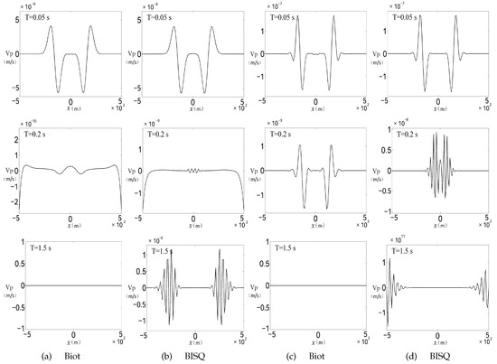
This test has all the numerical simulations with the different model solved by the stable finite-difference methods: the stable Biot model and the unstable BISQ model. The propagation of the seismic wave for a long time period can be observed: for T = 0.05 s the quick P-wave goes ahead, in T = 0.2 s, the quick P-wave reached and was absorbed by the boundary, the slow P-wave occurs, in T = 1.5 s, the slow P-wave reached, and was absorbed by the boundary. In the front of this procedure, the seismic waves calculated by different model and finite difference method are all propagating smoothly and entirely absorbed. However, the difference occurs from T = 0.2 s.

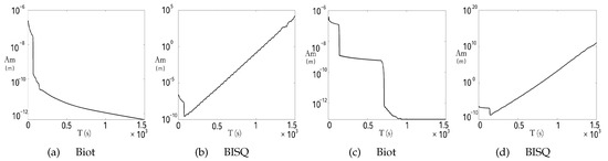
Figure 2 offers the amplitude (noted as Am) which changes as time (noted as T). By comparing (a) and (c) in Figure 1, it can be observed that the slow P-wave occurs only in the second-order scheme. The unstable phenomena only occur in the cases with the unstable BISQ model (see Figure 1b,d), in other words, the velocity occurs exponentially increasing phenomenon during the wave propagation. In the past numerical simulations, the little unstable phenomena such as those occurred in Figure 1d were often met and always attributed to the accuracy of the scheme and the boundary conditions. However, by observing Figure 1, it can be found that the instability of the numerical simulations due to the instability of the BISQ model. In addition, only for the cases in which time is large enough (such as T = 1.5 s), the unstable phenomenon which represented as the exponentially increasing amplitude as time can be significantly observed. Otherwise, the results calculated by the schemes (4)/(6)/(7) and (9)/(10)/(11) will be stable for the stable model (see (a) and (c) in Figure 1 and Figure 2). Even though there maybe some non-smooth solutions for the accuancy of the scheme, the amplitude also decreases to zero as time (see Figure 1a).

Above all, it is pointed out that the schemes (4)/(6)/(7) and (9)/(10)/(11) are applicable for the stable model. The schemes can be used to describe the wave propagation in a long time period. The characteristic boundary condition (4) can entirely absorb the waves. It is a convenient and effective boundary condition which can be easily combined with other models for wave propagation.

5. Conclusions

In this work, the stable theories in mathematics are introduced into the solutions of the wave propagation theories in geology and try to reconsider the calculated results from the point of view of stability instead of accuracy. The FD method with characteristic boundary conditions that confirm the overall-stability of the schemes is proposed. The stable conditions of this scheme obtained with the energy method in the context is important. Instead of the CFL conditions by the Fourier analysis method, it can be directly generated to the nonlinear elastic wave equations. The time-splitting method and characteristic boundary conditions are utilized in this approach. The time-splitting method reduces the computational complexity and the characteristic boundary conditions which are adjusted as the interior-points schemes can confirm the overall stability. Moreover, the schemes are applied to the Biot and BISQ models, and hence the numerical simulations show that the stable Biot model or the BISQ model in stable conditions can simulate wave propagations for a long time. This fact verifies the effectiveness of the FD method as a tool to detect the stability of arbitrary elastic wave modeling. In addition, the newly introduced characteristic boundary condition can vary to fit the FD method, and then it is feasible to combine it with other schemes in future.

References

- Burrascano, P.; Callegari, S.; Montisci, A.; Ricci, M.; Versaci, M. Ultrasonic Nondestructive Evaluation Systems: Industrial Application Issues; Springer: Berlin/Heidelberg, Germany, 2014. [Google Scholar]
- Guo, Z.; Xue, G.; Liu, J.; Wu, X. Electromagnetic methods for mineral exploration in China: A review. Ore Geol. Rev. 2020, 118, 103357. [Google Scholar]
- Versaci, M. Fuzzy approach and Eddy currents NDT/NDE devices in industrial applications. Electron. Lett. 2016, 52, 943–945. [Google Scholar] [CrossRef]
- Biot, M.A. Theory of propagation of elastic waves in a fluid-saturated porous solid. I. Low-frequency range. J. Acoust. Soc. Am. 1956, 28, 168–178. [Google Scholar] [CrossRef]
- Biot, M.A. Theory of propagation of elastic waves in a fluid-saturated porous solid. II. Higher frequency range. J. Acoust. Soc. Am. 1956, 28, 179–191. [Google Scholar] [CrossRef]
- Dvorkin, J.; Nur, A. Dynamic poroelasticity: A unified model with the squirt and the Biot mechanisms. Geophysics 1993, 58, 524–533. [Google Scholar] [CrossRef]
- Mavko, G.; Mukerji, T.; Dvorkin, J. The Rock Physics Handbook; Cambridge University Press: Cambridge, UK, 2020. [Google Scholar]
- Pan, X.; Zhang, G.; Yin, X. Azimuthally anisotropic elastic impedance inversion for fluid indicator driven by rock physics. Geophysics 2017, 82, C211–C227. [Google Scholar] [CrossRef]
- Yang, D.; Zhang, Z. Poroelastic wave equation including the Biot/squirt mechanism and the solid/fluid coupling anisotropy. Wave Motion 2002, 35, 223–245. [Google Scholar] [CrossRef]
- Carcione, J.M.; Gurevich, B. Differential form and numerical implementation of Biot’s poroelasticity equations with squirt dissipation. Geophysics 2011, 76, N55–N64. [Google Scholar] [CrossRef]
- Moczo, P.; Kristek, J.; Galis, M.; Pazak, P.; Balazovjech, M. The finite-difference and finite-element modeling of seismic wave propagation and earthquake motion. Acta Phys. Slovaca 2007, 57, 177–406. [Google Scholar] [CrossRef]
- Gauthier, O.; Virieux, J.; Tarantola, A. Two-dimensional nonlinear inversion of seismic waveforms: Numerical results. Geophysics 1986, 51, 1387–1403. [Google Scholar] [CrossRef]
- Virieux, J. P-SV wave propagation in heterogeneous media; velocity-stress finite-difference method. Geophysics 1986, 51, 889–901. [Google Scholar] [CrossRef]
- Igel, H.; Mora, P.; Riollet, B. Anisotropic wave propagation through finite-difference grids. Geophysics 1995, 60, 1203–1216. [Google Scholar] [CrossRef]
- Saenger, E.H.; Gold, N.; Shapiro, S.A. Modeling the propagation of elastic waves using a modified finite-difference grid. Wave Motion 2000, 31, 77–92. [Google Scholar] [CrossRef]
- Hustedt, B.; Operto, S.; Virieux, J. Mixed-grid and staggered-grid finite-difference methods for frequency-domain acoustic wave modelling. Geophys. J. Int. 2004, 157, 1269–1296. [Google Scholar] [CrossRef]
- Tian, X.F. Higher Order Time Difference Scheme and Stability Analysis for First-order Elastic Wave Staggered Grid; Coal geology of China, Taylor & Francis Online: Abingdon, UK, 2019; pp. 70–78. [Google Scholar]
- Yang, K.D.; Song, G.J.; Li, J.S. FCT compact difference simulation of wave propagation based on the Biot and the squirt-flow coupling interaction. Chin. J. Geophys. 2011, 54, 1348–1357. [Google Scholar]
- Liu, J.; Yong, W.A. Stability analysis of the Biot/squirt models for wave propagation in saturated porous media. Geophys. J. Int. 2016, 204, 535–543. [Google Scholar] [CrossRef]
- Yong, W.A. Boundary stabilization of hyperbolic balance laws with characteristic boundaries. Automatica 2019, 101, 252–257. [Google Scholar] [CrossRef]
- Zhu, Y.l.; Zhong, X.C.; Chen, B.M.; Zhang, Z.M. Difference Methods for Initial-Boundary-Value Problems and Flow Around Bodies; Springer Science & Business Media: Berlin/Heidelberg, Germany, 2013; Volume 4. [Google Scholar]
© 2020 by the authors. Licensee MDPI, Basel, Switzerland. This article is an open access article distributed under the terms and conditions of the Creative Commons Attribution (CC BY) license (http://creativecommons.org/licenses/by/4.0/).