Oscillatory Behavior of a Type of Generalized Proportional Fractional Differential Equations with Forcing and Damping Terms

Abstract

In this paper, we study the oscillatory behavior of solutions for a type of generalized proportional fractional differential equations with forcing and damping terms. Several oscillation criteria are established for the proposed equations in terms of Riemann-Liouville and Caputo settings. The results of this paper generalize some existing theorems in the literature. Indeed, it is shown that for particular choices of parameters, the obtained conditions in this paper reduce our theorems to some known results. Numerical examples are constructed to demonstrate the effectiveness of the our main theorems. Furthermore, we present and illustrate an example which does not satisfy the assumptions of our theorem and whose solution demonstrates nonoscillatory behavior.

1. Introduction

Fractional calculus is a mathematical branch investigating the properties of derivatives and integrals of non-integer orders. The significance of this subject falls in the fact that the fractional derivative has the feature of nonlocal nature. This property makes these derivatives suitable to simulate more physical phenomena such as earthquake vibrations, polymers, and so forth; see, for example, References [1,2,3,4,5,6,7,8,9,10] and the references cited therein.

In recent years, there have appeared different types of fractional derivatives. However, it has been realized that most of these derivatives lose some of their basic properties that classical derivatives have such as the product rule and the chain rule. Fortunately, Khalil et al. [11] defined a new well-behaved fractional derivative, called the “conformable fractional derivative”, which depends entirely on the classical limit definition of the derivative. Thereafter, researchers developed the conformable derivative and obtained different results exposing its features [12,13,14]. Recently, Jarad et al. [15] introduced the generalized proportional fractional (GPF) derivative of Caputo and Riemann-Liouville type involving exponential functions in their kernels. The GPF derivative not only preserves classical properties but also verifies semi group property and of nonlocal behavior. For recent results involving GPF derivative, one can refer to References [16,17,18].

In 2012, Grace et al. [19] initiated the study of oscillation theory for fractional differential equations. Thereafter, many researchers have investigated the oscillatory properties of fractional differential equations; see for instance References [20,21,22,23,24,25]. In 2019, Aphithana et al. [24] studied forced oscillatory properties of solutions to the conformable initial value problem of the form

$$\begin{array}{c}\hfill \left\{\begin{array}{c}{}_a{D}^{1+\alpha ,\rho }x\left(t\right)+p\left(t\right){}_a{D}^{\alpha ,\rho }x\left(t\right)+q\left(t\right)f\left(x\left(t\right)\right)=g\left(t\right),t>a,\hfill \\ \underset{t\to a^{+}}{lim}{}_a{\mathcal{J}}^{j-\alpha ,\rho }x\left(t\right)=b_j(j=1,2,\dots ,m),\hfill \end{array}\right.\end{array}$$

where $m=\lceil \alpha \rceil$, $0<\rho \le 1$,p, $g\in \mathbb{C}({\mathbb{R}}^{+},\mathbb{R})$, $q\in \mathbb{C}({\mathbb{R}}^{+},{\mathbb{R}}^{+})$, $f\in \mathbb{C}(\mathbb{R},\mathbb{R})$ are continuous functions, ${}_a{D}^{\alpha ,\rho }$ is the left conformable derivative of order $\alpha \in \mathbb{C}$ of x, $Re\left(\alpha \right)\ge 0$ in the Riemann-Liouville setting and ${}_a{\mathcal{J}}^{j-\alpha ,\rho }$ is the left conformable integral operator of order $j-\alpha \in \mathbb{C}$, $b_j\in \mathbb{R}$, $j=1,2,\dots ,m$.

They also studied the forced oscillation of conformable initial value problems in the Caputo setting of the form

$$\begin{array}{c}\hfill \left\{\begin{array}{c}{}_a^C{D}^{1+\alpha ,\rho }x\left(t\right)+p\left(t\right){}_a^C{D}^{\alpha ,\rho }x\left(t\right)+q\left(t\right)f\left(x\left(t\right)\right)=g\left(t\right),t>a,\hfill \\ {}_a^k{D}^{\rho }x\left(a\right)=b_k(k=0,1,\dots ,m-1),\hfill \end{array}\right.\end{array}$$

where $m=\lceil \alpha \rceil$, $0<\rho \le 1$, and ${}_a^C{D}^{\alpha ,\rho }$ is the left conformable derivative of order $\alpha \in \mathbb{C}$ of x, $Re\left(\alpha \right)\ge 0$ in the Caputo setting.

In 2020, Sudsutad et al. [26] established some oscillation criteria for the following generalized proportional fractional differential equation

$$\begin{array}{c}\hfill \left\{\begin{array}{c}{}_a{D}^{\alpha ,\rho }x\left(t\right)+{\xi }_1(t,x\left(t\right))=\mu \left(t\right)+{\xi }_2(t,x\left(t\right)),t>a\ge 0,\hfill \\ \underset{t\to a^{+}}{lim}{}_a{I}^{j-\alpha ,\rho }x\left(t\right)=b_j(j=1,2,\dots ,n),\hfill \end{array}\right.\end{array}$$

with $n=\lceil \alpha \rceil$, ${}_a{D}^{\alpha ,\rho }$ is the generalized proportional fractional derivative operator of order $\alpha \in \mathbb{C}$, $Re\left(\alpha \right)\ge 0$, $0<\rho \le 1$ in the Riemann-Liouville setting and ${}_a{I}^{\alpha ,\rho }$ is the generalized proportional fractional integral operator.

In this paper, motivated by the above papers, we establish some sufficient conditions for forced oscillation criteria of all solutions of the generalized proportional fractional (GPF) initial value problem with damping term in the Riemann-Liouville type of the form:

$$\begin{array}{c}\hfill \left\{\begin{array}{c}{}_a{D}^{1+\alpha ,\rho }y\left(l\right)+p\left(l\right){}_a{D}^{\alpha ,\rho }y\left(l\right)+q\left(l\right)f\left(y\left(l\right)\right)=g\left(l\right),l>a\ge 0,\hfill \\ \underset{l\to a^{+}}{lim}{}_a{I}^{j-\alpha ,\rho }y\left(l\right)=b_j(j=1,2,\dots ,m),\hfill \end{array}\right.\end{array}$$

(1)

where $m=\lceil \alpha \rceil$, $0<\rho \le 1$, ${}_a{D}^{\alpha ,\rho }$ is the left GPF derivative of order $\alpha \in \mathbb{C}$ of y, $Re\left(\alpha \right)\ge 0$ in the Riemann-Liouville setting and ${}_a{I}^{j-\alpha ,\rho }$ is the left GPF integral of order $j-\alpha \in \mathbb{C}$, $Re(j-\alpha )>0$, $b_j\in \mathbb{R}$, $j=1,2,\dots ,m$ and p, $g\in \mathbb{C}({\mathbb{R}}^{+},\mathbb{R})$, $q\in \mathbb{C}({\mathbb{R}}^{+},{\mathbb{R}}^{+})$, $f\in \mathbb{C}(\mathbb{R},\mathbb{R})$.

Moreover, we study the forced oscillation criteria of all solutions of the GPF initial value problem with damping term in the Caputo type of the form

$$\begin{array}{c}\hfill \begin{array}{c}{}_a^C{D}^{1+\alpha ,\rho }y\left(l\right)+p\left(l\right){}_a^C{D}^{\alpha ,\rho }y\left(l\right)+q\left(l\right)f\left(y\left(l\right)\right)=g\left(l\right),l>a\ge 0,\hfill \\ D^{k,\rho }y\left(a\right)=b_k(k=0,1,\dots ,n-1),\hfill \end{array}\end{array}$$

(2)

where $n=\lceil \alpha \rceil$, $0<\rho \le 1$, ${}_a^C{D}^{\alpha ,\rho }$ is the left GPF derivative of order $\alpha \in \mathbb{C}$ of y, $Re\left(\alpha \right)\ge 0$ in the Caputo setting and $D^{k,\rho }={\underbrace{D^{\rho }{D}^{\rho }\cdots D^{\rho }}}_{\mathrm{k}\mathrm{times}}$, and $D^{\rho }$ is the proportional derivative defined in Reference [13].

We claim that the results of this paper improve and generalize previously existing oscillation results in Reference [24].

Definition 1.

The solution y of problem (1) (respectively (2)) is called oscillatory if it has arbitrarily large zeros on $(0,\infty )$; otherwise, it is called nonoscillatory. An equation is called oscillatory if all its solutions are oscillatory.

2. Preliminaries

In this section, we provide some basic definitions and results which will be used throughout this paper. For the justifications and proofs, the reader can consult References [13,15].

Definition 2.

[15] (Modified Conformable Derivatives).

For $\rho \in [0,1]$, let the functions $k_0,k_1:[0,1]\times \mathbb{R}\to [0,\infty )$ be continuous such that for all $l\in \mathbb{R}$ we have

$$\underset{\rho \to 0^{+}}{lim}{k}_1(\rho ,l)=1,\underset{\rho \to 0^{+}}{lim}{k}_0(\rho ,l)=0,\underset{\rho \to 1^{-}}{lim}{k}_1(\rho ,l)=0,\underset{\rho \to 1^{-}}{lim}{k}_0(\rho ,l)=1,$$

(3)

and $k_1(\rho ,l)\ne 0$, $\rho \in [0,1)$, $k_0(\rho ,l)\ne 0$, $\rho \in (0,1]$.

Then, Anderson et al. [13] defined the modified conformable differential operator of order $\rho$ by

$$D^{\rho }f\left(l\right)=k_1(\rho ,l)f\left(l\right)+k_0(\rho ,l)f^{\prime }\left(l\right),$$

(4)

provided that the right-hand side exists at $l\in \mathbb{R}$ and $f^{\prime }\left(l\right)=\frac{d}{dl}f.$ The derivative given in (4) is called a proportional derivative. For more details about the control theory of the proportional derivatives and its component functions ${\mathit{k}}_{\mathit{0}}$ and ${\mathit{k}}_{\mathit{1}}$, we refer the reader to [27].

Of special interest, we shall restrict ourselves to the case when $k_1(\rho ,l)=(1-\rho )$ and $k_0(\rho ,l)=\rho$. Therefore, (4) becomes

$$D^{\rho }f\left(l\right)=(1-\rho )f\left(l\right)+\rho f^{\prime }\left(l\right).$$

(5)

Notice that $\underset{\rho \to 0^{+}}{lim}{D}^{\rho }f\left(l\right)=f\left(l\right)$ and $\underset{\rho \to 1^{-}}{lim}{D}^{\rho }f\left(l\right)=f^{\prime }\left(l\right)$. It is clear that the derivative (5) is somehow more general than the conformable derivative which does not tend to the original function as $\rho$ tends to 0.

To find the associated integral to the proportional derivative in (5), we solve the following equation

$$D^{\rho }g\left(l\right)=(1-\rho )g\left(l\right)+\rho g^{\prime }\left(l\right)=f\left(l\right),l\ge a.$$

The above equation is a first order linear differential equation and its solution is given by

$$g\left(l\right)=\frac{1}{\rho }{\int }_a^l{e}^{\frac{\rho -1}{\rho }(l-s)}f\left(s\right)ds.$$

Define the proportional integral associated to $D^{\rho }$ by

$${}_a{I}^{1,\rho }f\left(l\right)=\frac{1}{\rho }{\int }_a^l{e}^{\frac{\rho -1}{\rho }(l-s)}f\left(s\right)ds,$$

(6)

where we accept that ${}_a{I}^{0,\rho }f\left(l\right)=f\left(l\right).$

Lemma 1.

[15] Let f be defined on $[a,\infty )$ and differentiable on $(a,\infty )$ and $\rho \in (0,1]$. Then, we have

$${}_a{I}^{1,\rho }{D}^{\rho }f\left(l\right)=f\left(l\right)-e^{\frac{\rho -1}{\rho }(l-a)}f\left(a\right).$$

(7)

Definition 3.

[15] For $\rho \in (0,1]$ and $\alpha \in \mathbb{C}$, $Re\left(\alpha \right)>0,$ we define the left GPF integral of f by

$$\begin{array}{c}\hfill \left({}_a{I}^{\alpha ,\rho }f\right)\left(l\right)=\frac{1}{{\rho }^{\alpha }\Gamma \left(\alpha \right)}{\int }_a^l{e}^{\frac{\rho -1}{\rho }(l-s)}{(l-s)}^{\alpha -1}f\left(s\right)ds={\rho }^{-\alpha }{e}^{\frac{\rho -1}{\rho }l}{}_a{I}^{\alpha }\left(e^{\frac{1-\rho }{\rho }l}f\left(l\right)\right),\end{array}$$

(8)

where ${}_a{I}^{\alpha }$ is the left Riemann-Liouville fractional integral of order α.

The right GPF integral ending at b, however, can be defined by

$$\begin{array}{c}\hfill \left(I_b^{\alpha ,\rho }f\right)\left(l\right)=\frac{1}{{\rho }^{\alpha }\Gamma \left(\alpha \right)}{\int }_l^b{e}^{\frac{\rho -1}{\rho }(s-l)}{(s-l)}^{\alpha -1}f\left(s\right)ds={\rho }^{-\alpha }{e}^{\frac{\rho -1}{\rho }l}{I}_b^{\alpha }\left(e^{\frac{1-\rho }{\rho }l}f\left(l\right)\right),\end{array}$$

(9)

where $I_b^{\alpha }$ is the right Riemann-Liouville fractional integral of order α.

Definition 4.

[15] For $\rho \in (0,1]$ and $\alpha \in \mathbb{C}$, $Re\left(\alpha \right)\ge 0,$ we define the left GPF derivative of f by

$$\begin{array}{cc}\hfill \left({}_a{D}^{\alpha ,\rho }f\right)\left(l\right)& =D^{n,\rho }{}_a{I}^{n-\alpha ,\rho }f\left(l\right)\hfill \\ & =\frac{D_l^{n,\rho }}{{\rho }^{n-\alpha }\Gamma (n-\alpha )}{\int }_a^l{e}^{\frac{\rho -1}{\rho }(l-s)}{(l-s)}^{n-\alpha -1}f\left(s\right)ds.\hfill \end{array}$$

(10)

The right GPF derivative ending at b is defined by

$$\begin{array}{cc}\hfill \left(D_b^{\alpha ,\rho }f\right)\left(l\right)& ={}_{\ominus }{D}^{n,\rho }{I}_b^{n-\alpha ,\rho }f\left(l\right)\hfill \\ & =\frac{{}_{\ominus }{D}_l^{n,\rho }}{{\rho }^{n-\alpha }\Gamma (n-\alpha )}{\int }_l^b{e}^{\frac{\rho -1}{\rho }(s-l)}{(s-l)}^{n-\alpha -1}f\left(s\right)ds,\hfill \end{array}$$

(11)

where $n=\left[Re\right(\alpha \left)\right]+1$.

If we let $\rho =1$ in Definition 4, then one can obtain the left and right Riemann-Liouville fractional derivatives as in [6]. Moreover, it is clear that

$$\underset{\alpha \to 0}{lim}{D}^{\alpha ,\rho }f\left(l\right)=f\left(l\right)\mathrm{and}\underset{\alpha \to 1}{lim}{D}^{\alpha ,\rho }f\left(l\right)=D^{\rho }f\left(l\right).$$

Lemma 2.

[15] Let $Re\left(\alpha \right)>0,$ $n=-[-Re(\alpha \left)\right],$ $f\in L_1(a,b)$ and $\left({}_a{I}^{\alpha ,\rho }f\right)\left(l\right)\in A{C}^n[a,b].$ Then,

$$\begin{array}{c}\hfill \left({}_a{I}^{\alpha ,\rho }{}_a{D}^{\alpha ,\rho }f\right)\left(l\right)=f\left(l\right)-e^{\frac{\rho -1}{\rho }(l-a)}\sum _{j=1}^n\left({}_a{I}^{j-\alpha ,\rho }f\right)\left(a^{+}\right)\frac{{(l-a)}^{\alpha -j}}{{\rho }^{\alpha -j}\Gamma (\alpha +1-j)}.\end{array}$$

(12)

Definition 5.

[13] (Partial Conformable Derivatives). Let $\rho \in [0,1]$, and let the functions $k_0,k_1:[0,1]\times \mathbb{R}\to [0,\infty )$ be continuous and satisfy (3). Given a function $f:{\mathbb{R}}^2\to \mathbb{R}$ such that $\frac{\partial }{\partial l}f(l,s)$ exists for each fixed $s\in \mathbb{R}$, define the partial differential operator $D_l^{\rho }$ via

$$D_l^{\rho }f(l,s)=k_1(\rho ,l)f(l,s)+k_0(\rho ,l)\frac{\partial }{\partial l}f(l,s).$$

(13)

Definition 6.

[13] (Conformable Exponential Function). Let $\rho \in (0,1]$, the points $s,l,\in \mathbb{R}$ with $s\le l$, and let the function $p:[s,l]\to \mathbb{R}$ be continuous. Let $k_0,k_1:[0,1]\times \mathbb{R}\to [0,\infty )$ be continuous and satisfy (3), with $p/k_0$ and $k_1/k_0$ Riemann integrable on $[s,l]$. Then the exponential function with respect to $D^{\rho }$ in (4) is defined to be

$$e_p(l,s):=e^{{\int }_s^l\frac{p\left(\tau \right)-k_1(\rho ,\tau )}{k_0(\rho ,\tau )}d\tau },e_0(l,s):=e^{-{\int }_s^l\frac{k_1(\rho ,\tau )}{k_0(\rho ,\tau )}d\tau }.$$

(14)

Using (4) and (14), we have the following basic results.

Lemma 3.

[13] (Basic Derivatives). Let the conformable differential operator $D^{\rho }$ be given as in (4), where $\rho \in [0,1]$. Let the function $p:[s,l]\to \mathbb{R}$ be continuous. Let $k_0,k_1:[0,1]\times \mathbb{R}\to [0,\infty )$ be continuous and satisfy (3), with $p/k_0$ and $k_1/k_0$ Riemann integrable on $[s,l]$. Assume the functions f and g are differentiable as needed. Then

$\left(i\right)$

$D^{\rho }[af+bg]=a{D}^{\rho }\left[f\right]+b{D}^{\rho }\left[g\right]for alla,b\in \mathbb{R}$;

$\left(ii\right)$

$D^{\rho }c=c{k}_1(\rho ,)for all constantsc\in \mathbb{R}$;

$\left(iii\right)$

$D^{\rho }\left[fg\right]=f{D}^{\rho }\left[g\right]+g{D}^{\rho }\left[f\right]-fg{k}_1(\rho ,)$;

$\left(iv\right)$

$D^{\rho }[f/g]=\frac{g{D}^{\rho }\left[f\right]-f{D}^{\rho }\left[g\right]}{g^2}+\frac{f}{g}{k}_1(\rho ,)$;

$\left(v\right)$

for $\rho \in (0,1]$ and fixed $s\in \mathbb{R}$, the exponential function satisfies

$$D_l^{\rho }\left[e_p(l,s)\right]=p\left(l\right)e_p(l,s)$$

for $e_p(l,s)$ given in (14);

$\left(vi\right)$

for $\rho \in (0,1]$ and for the exponential function $e_0$ given in (14), we have

$$D^{\rho }\left[{\int }_a^l\frac{f\left(s\right)e_0(l,s)}{k_0(\rho ,s)}ds\right]=f\left(l\right).$$

Definition 7.

[15] For $\rho \in (0,1]$ and $\alpha \in \mathbb{C}$ with $Re\left(\alpha \right)\ge 0$, we define the left GPF derivative of Caputo type starting at a by

$$\begin{array}{cc}\hfill \left({}_a^C{D}^{\alpha ,\rho }f\right)\left(l\right)& ={}_a{I}^{n-\alpha ,\rho }\left(D^{n,\rho }f\right)\left(l\right)\hfill \\ & =\frac{1}{{\rho }^{n-\alpha }\Gamma (n-\alpha )}{\int }_a^l{e}^{\frac{\rho -1}{\rho }(l-s)}{(l-s)}^{n-\alpha -1}\left(D^{n,\rho }f\right)\left(s\right)ds.\hfill \end{array}$$

(15)

The right GPF derivative of Caputo ending at b is defined by

$$\begin{array}{cc}\hfill \left({}^C{D}_b^{\alpha ,\rho }f\right)\left(l\right)& =I_b^{n-\alpha ,\rho }{(}_{\ominus }{D}^{n,\rho }f)\left(l\right)\hfill \\ & =\frac{1}{{\rho }^{n-\alpha }\Gamma (n-\alpha )}{\int }_l^b{e}^{\frac{\rho -1}{\rho }(s-l)}{(s-l)}^{n-\alpha -1}{(}_{\ominus }{D}^{n,\rho }f)\left(s\right)ds,\hfill \end{array}$$

(16)

where $n=\left[Re\right(\alpha \left)\right]+1$.

Lemma 4.

[15] For $\rho \in (0,1]$ and $n=\left[Re\right(\alpha \left)\right]+1$, we have

$${}_a{I}^{\alpha ,\rho }\left({}_a^C{D}^{\alpha ,\rho }f\right)\left(l\right)=f\left(l\right)-\sum _{k=0}^{n-1}\frac{\left(D^{k,\rho }f\right)\left(a\right)}{{\rho }^{k}k!}{(l-a)}^k{e}^{\frac{\rho -1}{\rho }}(l-a).$$

(17)

Proposition 1.

[15] Let $\alpha ,\beta \in \mathbb{C}$ be such that $Re\left(\alpha \right)\ge 0$ and $Re\left(\beta \right)>0$. Then, for any $0<\rho \le 1$ and $n=\left[Re\right(\alpha \left)\right]+1$, we have

(i) 

$\left({{}_{a}I}^{\alpha ,\rho }{e}^{\frac{\rho -1}{\rho }l}{(l-a)}^{\beta -1}\right)\left(y\right)=\frac{\Gamma \left(\beta \right)}{\Gamma (\beta +\alpha ){\rho }^{\alpha }}{e}^{\frac{\rho -1}{\rho }y}{(y-a)}^{\beta +\alpha -1},Re\left(\alpha \right)>0.$

(ii) 

$\left({{}_{a}D}^{\alpha ,\rho }{e}^{\frac{\rho -1}{\rho }l}{(l-a)}^{\beta -1}\right)\left(y\right)=\frac{{\rho }^{\alpha }\Gamma \left(\beta \right)}{\Gamma (\beta -\alpha )}{e}^{\frac{\rho -1}{\rho }y}{(y-a)}^{\beta -\alpha -1},Re\left(\alpha \right)\ge 0.$

(iii) 

$\left({{}_a^{C}D}^{\alpha ,\rho }{e}^{\frac{\rho -1}{\rho }l}{(l-a)}^{\beta -1}\right)\left(y\right)=\frac{{\rho }^{\alpha }\Gamma \left(\beta \right)}{\Gamma (\beta -\alpha )}{e}^{\frac{\rho -1}{\rho }y}{(y-a)}^{\beta -\alpha -1},Re\left(\alpha \right)>n.$

3. Oscillation Results via Riemann-Liouville Operator

In this section, we establish the oscillation criteria for the GPF initial value problem (1). We prove our results under the following assumption:

$\left(H\right)$

$p\in \mathbb{C}({\mathbb{R}}^{+},\mathbb{R})$, $q\in \mathbb{C}({\mathbb{R}}^{+},{\mathbb{R}}^{+})$, $g\in \mathbb{C}({\mathbb{R}}^{+},\mathbb{R})$, $f\in C(\mathbb{R},\mathbb{R})$ with $\frac{f\left(u\right)}{u}>0$ for all $u\ne 0$.

For our convenience, we set the following notations:

$$\begin{array}{ccc}\hfill \Phi \left(l\right)& :=& \Gamma \left(\alpha \right)e^{\frac{\rho -1}{\rho }(l-a)}\sum _{j=1}^m\frac{{\rho }^j{b}_j{(l-a)}^{\alpha -j}}{\Gamma (\alpha +1-j)},\hfill \end{array}$$

(18)

$$\begin{array}{ccc}\hfill \Lambda (l,L)& :=& {\int }_a^L{e}^{\frac{\rho -1}{\rho }(l-s)}{(l-s)}^{\alpha -1}\left(\frac{e^{\frac{\rho -1}{\rho }(s-l_1)}M+{}_{l_1}{I}^{1,\rho }\left(\rho g\left(s\right)V\left(s\right)\right)}{V\left(s\right)}\right)ds,\hfill \end{array}$$

(19)

$$\begin{array}{ccc}\hfill V\left(l\right)& :=& exp{\int }_{l_1}^l\frac{\rho p\left(\tau \right)-(1-\rho )}{\rho }d\tau ,\hfill \end{array}$$

(20)

$$\begin{array}{ccc}\hfill M& :=& {}_{l_1}{D}^{\alpha ,\rho }y\left(l_1\right)V\left(l_1\right),M\mathrm{is}\mathrm{an}\mathrm{arbitrary}\mathrm{constant}.\hfill \end{array}$$

(21)

Theorem 1.

Assume that $\left(H\right)$ holds. If

$$\begin{array}{c}\hfill \underset{l\to \infty }{lim}inf{l}^{1-\alpha }{\int }_L^l{e}^{\frac{\rho -1}{\rho }(l-s)}{(l-s)}^{\alpha -1}\left[\frac{e^{\frac{\rho -1}{\rho }(s-l_1)}M+{}_{l_1}{I}^{1,\rho }\left(\rho g\left(s\right)V\left(s\right)\right)}{V\left(s\right)}\right]ds=-\infty \end{array}$$

(22)

and

$$\begin{array}{c}\hfill \underset{l\to \infty }{lim}sup{l}^{1-\alpha }{\int }_L^l{e}^{\frac{\rho -1}{\rho }(l-s)}{(l-s)}^{\alpha -1}\left[\frac{e^{\frac{\rho -1}{\rho }(s-l_1)}M+{}_{l_1}{I}^{1,\rho }\left(\rho g\left(s\right)V\left(s\right)\right)}{V\left(s\right)}\right]ds=\infty ,\end{array}$$

(23)

for every sufficiently large L, where $V\left(l\right)$ and M are defined as in (20) and (21) respectively, then every solution of problem (1) is oscillatory.

Proof. 

Suppose that $y\left(l\right)$ is a nonoscillatory solution of problem (1). Without loss of generality, let $L>a$ be large enough and $l_1\ge L$ such that $y\left(l\right)>0$ for all $l\ge l_1$. Using Lemma 3 (iii), Equations (5) and (13), we have

$$\begin{array}{cc}\hfill D^{\rho }{[}_a{D}^{\alpha ,\rho }y\left(l\right)V\left(l\right)]& ={}_a{D}^{\alpha ,\rho }y\left(l\right)D^{\rho }V\left(l\right)+V\left(l\right)D^{\rho }\left({}_a{D}^{\alpha ,\rho }y\left(l\right)\right)-(1-\rho ){}_a{D}^{\alpha ,\rho }y\left(l\right)V\left(l\right)\hfill \\ & ={}_a{D}^{\alpha ,\rho }y\left(l\right)D^{\rho }V\left(l\right)+V\left(l\right)\left[(1-\rho ){}_a{D}^{\alpha ,\rho }y\left(l\right)+\rho \frac{d}{dl}\left({}_a{D}^{\alpha ,\rho }y\left(l\right)\right)\right]\hfill \\ & -(1-\rho ){}_a{D}^{\alpha ,\rho }y\left(l\right)V\left(l\right)\hfill \\ & =\rho \left[{}_a{D}^{1+\alpha ,\rho }y\left(l\right)+p\left(l\right){}_a{D}^{\alpha ,\rho }y\left(l\right)\right]V\left(l\right)\hfill \\ & =\rho \left[-q\left(l\right)f\left(y\right(l\left)\right)+g\left(l\right)\right]V\left(l\right)\hfill \\ & <\rho g\left(l\right)V\left(l\right).\hfill \end{array}$$

Taking the proportional integral operator ${}_{l_1}{I}^{1,\rho }$ on both sides to the above inequality, we obtain

$${}_{l_1}{I}^{1,\rho }\left(D^{\rho }\left[{}_a{D}^{\alpha ,\rho }y\left(l\right)V\left(l\right)\right]\right)<{}_{l_1}{I}^{1,\rho }\left(\rho g\left(l\right)V\left(l\right)\right).$$

(24)

Using Lemma 1 on the L.H.S of (24), we have

$${}_a{D}^{\alpha ,\rho }y\left(l\right)<\frac{e^{\frac{\rho -1}{\rho }(l-l_1)}M+{}_{l_1}{I}^{1,\rho }\left(\rho g\left(l\right)V\left(l\right)\right)}{V\left(l\right)}.$$

Taking the left GPF integral operator ${}_a{I}^{\alpha ,\rho }$ on both sides to the above inequality, we get

$${}_a{I}^{\alpha ,\rho }\left({}_a{D}^{\alpha ,\rho }y\left(l\right)\right)<{}_a{I}^{\alpha ,\rho }\left[\frac{e^{\frac{\rho -1}{\rho }(l-l_1)}M+{}_{l_1}{I}^{1,\rho }\left(\rho g\left(l\right)V\left(l\right)\right)}{V\left(l\right)}\right].$$

(25)

Using Lemma 2 on the L.H.S of (25), we have

$$y\left(l\right)-e^{\frac{\rho -1}{\rho }(l-a)}\sum _{j=1}^m\frac{b_j{(l-a)}^{\alpha -j}}{{\rho }^{\alpha -j}\Gamma (\alpha +1-j)}<{}_a{I}^{\alpha ,\rho }\left[\frac{e^{\frac{\rho -1}{\rho }(l-l_1)}M+{}_{l_1}{I}^{1,\rho }\left(\rho g\left(l\right)V\left(l\right)\right)}{V\left(l\right)}\right].$$

(26)

Applying the left GPF integral formula on the R.H.S of (26), we have

$$\begin{array}{cc}\hfill y\left(l\right)& <e^{\frac{\rho -1}{\rho }(l-a)}\sum _{j=1}^m\frac{b_j{(l-a)}^{\alpha -j}}{{\rho }^{\alpha -j}\Gamma (\alpha +1-j)}\hfill \\ & +\frac{1}{{\rho }^{\alpha }\Gamma \left(\alpha \right)}{\int }_a^l{e}^{\frac{\rho -1}{\rho }(l-s)}{(l-s)}^{\alpha -1}\left[\frac{e^{\frac{\rho -1}{\rho }(s-l_1)}M+{}_{l_1}{I}^{1,\rho }\left(\rho g\left(s\right)V\left(s\right)\right)}{V\left(s\right)}\right]ds,\hfill \end{array}$$

for every sufficiently large L. If we multiply the above inequality by ${\rho }^{\alpha }\Gamma \left(\alpha \right)$, we get

$$\begin{array}{cc}\hfill {\rho }^{\alpha }\Gamma \left(\alpha \right)y\left(l\right)& <\Gamma \left(\alpha \right)e^{\frac{\rho -1}{\rho }(l-a)}\sum _{j=1}^m\frac{{\rho }^j{b}_j{(l-a)}^{\alpha -j}}{\Gamma (\alpha +1-j)}\hfill \\ & +{\int }_a^L{e}^{\frac{\rho -1}{\rho }(l-s)}{(l-s)}^{\alpha -1}\left[\frac{e^{\frac{\rho -1}{\rho }(s-l_1)}M+{}_{l_1}{I}^{1,\rho }\left(\rho g\left(s\right)V\left(s\right)\right)}{V\left(s\right)}\right]ds\hfill \\ & +{\int }_L^l{e}^{\frac{\rho -1}{\rho }(l-s)}{(l-s)}^{\alpha -1}\left[\frac{e^{\frac{\rho -1}{\rho }(s-l_1)}M+{}_{l_1}{I}^{1,\rho }\left(\rho g\left(s\right)V\left(s\right)\right)}{V\left(s\right)}\right]ds\hfill \\ & =\Phi \left(l\right)+\Lambda (l,L)+{\int }_L^l{e}^{\frac{\rho -1}{\rho }(l-s)}{(l-s)}^{\alpha -1}\left[\frac{e^{\frac{\rho -1}{\rho }(s-l_1)}M+{}_{l_1}{I}^{1,\rho }\left(\rho g\left(s\right)V\left(s\right)\right)}{V\left(s\right)}\right]ds,\hfill \end{array}$$

(27)

where $\Phi \left(l\right)$ and $\Lambda (l,L)$ are defined in (18) and (19), respectively.

Multiplying (27) by $l^{1-\alpha }$, we get

$$\begin{array}{cc}\hfill 0& <l^{1-\alpha }{\rho }^{\alpha }\Gamma \left(\alpha \right)y\left(l\right)\hfill \\ & <l^{1-\alpha }\Phi \left(l\right)+l^{1-\alpha }\Lambda (l,L)\hfill \\ & +l^{1-\alpha }{\int }_L^l{e}^{\frac{\rho -1}{\rho }(l-s)}{(l-s)}^{\alpha -1}\left[\frac{e^{\frac{\rho -1}{\rho }(s-l_1)}M+{}_{l_1}{I}^{1,\rho }\left(\rho g\left(s\right)V\left(s\right)\right)}{V\left(s\right)}\right]ds.\hfill \end{array}$$

(28)

Let us consider the following two cases for $L_1\ge L$.

Case(i): Let $0<\alpha \le 1$. Then $m=1$. Since $\left|e^{\frac{\rho -1}{\rho }(l-a)}\right|\le 1$ and the function $h_1\left(l\right)={\left(\frac{l-a}{l}\right)}^{\alpha -1}$ is decreasing for $\rho >0$, $0<\alpha <1$, we get for $l\ge L_1$,

$$\begin{array}{c}\hfill \left|l^{1-\alpha }\Phi \left(l\right)\right|=\left|e^{\frac{\rho -1}{\rho }(l-a)}\rho b_1{\left(\frac{l-a}{l}\right)}^{\alpha -1}\right|\le \rho \left|b_1\right|{\left(\frac{L_1-a}{L_1}\right)}^{\alpha -1}:=C_1\left(L_1\right),\end{array}$$

(29)

and

$$\begin{array}{cc}\hfill \left|l^{1-\alpha }\Lambda (l,L)\right|& =\left|l^{1-\alpha }{\int }_a^L{e}^{\frac{\rho -1}{\rho }(l-s)}{(l-s)}^{\alpha -1}\left(\frac{e^{\frac{\rho -1}{\rho }(s-l_1)}M+{}_{l_1}{I}^{1,\rho }\left(\rho g\left(s\right)V\left(s\right)\right)}{V\left(s\right)}\right)ds\right|\hfill \\ & \le {\int }_a^L\left|e^{\frac{\rho -1}{\rho }(l-s)}\right|{\left(\frac{l-a}{l}\right)}^{\alpha -1}\left|\frac{e^{\frac{\rho -1}{\rho }(s-l_1)}M+{}_{l_1}{I}^{1,\rho }\left(\rho g\left(s\right)V\left(s\right)\right)}{V\left(s\right)}\right|ds\hfill \\ & \le {\int }_a^L{\left(\frac{L_1-a}{L_1}\right)}^{\alpha -1}\left|\frac{e^{\frac{\rho -1}{\rho }(s-l_1)}M+{}_{l_1}{I}^{1,\rho }\left(\rho g\left(s\right)V\left(s\right)\right)}{V\left(s\right)}\right|ds\hfill \\ & :=C_2(L,L_1).\hfill \end{array}$$

(30)

From (28), (29) and (30), we get, for $l\ge L_1$,

$$l^{1-\alpha }{\int }_L^l{e}^{\frac{\rho -1}{\rho }(l-s)}{(l-s)}^{\alpha -1}\left[\frac{e^{\frac{\rho -1}{\rho }(s-l_1)}M+{}_{l_1}{I}^{1,\rho }\left(\rho g\left(s\right)V\left(s\right)\right)}{V\left(s\right)}\right]ds\ge -[C_1\left(L_1\right)+C_2(L,L_1)].$$

Since the R.H.S of the above inequality is a negative constant, it follows that

$$\underset{l\to \infty }{lim}inf{l}^{1-\alpha }{\int }_L^l{e}^{\frac{\rho -1}{\rho }(l-s)}{(l-s)}^{\alpha -1}\left[\frac{e^{\frac{\rho -1}{\rho }(s-l_1)}M+{}_{l_1}{I}^{1,\rho }\left(\rho g\left(s\right)V\left(s\right)\right)}{V\left(s\right)}\right]ds>-\infty ,$$

which leads to a contradiction with (22).

Case(ii): Let $\alpha >1$. Then $m\ge 2$ and ${\left(\frac{l-a}{l}\right)}^{\alpha -1}<1$ for $\alpha >1$ and $\rho >0$. Since $\left|e^{\frac{\rho -1}{\rho }(l-a)}\right|\le 1$ and the function $h_2\left(l\right)={(l-a)}^{1-j}$ is decreasing for $j>1$ and $\rho >0$, for $l\ge L_1$, we have

$$\begin{array}{cc}\hfill \left|l^{1-\alpha }\Phi \left(l\right)\right|& =\left|l^{1-\alpha }\Gamma \left(\alpha \right)e^{\frac{\rho -1}{\rho }(l-a)}\sum _{j=1}^m\frac{{\rho }^j{b}_j{(l-a)}^{\alpha -j}}{\Gamma (\alpha +1-j)}\right|\hfill \\ & \le \Gamma \left(\alpha \right){\left(\frac{l-a}{l}\right)}^{\alpha -1}\sum _{j=1}^m\frac{{\rho }^j\left|b_j\right|{(l-a)}^{1-j}}{\Gamma (\alpha +1-j)}\hfill \\ & \le \Gamma \left(\alpha \right)\sum _{j=1}^m\frac{{\rho }^j\left|b_j\right|{(L_1-a)}^{1-j}}{\Gamma (\alpha +1-j)}\hfill \\ & :=C_3\left(L_1\right),\hfill \end{array}$$

(31)

and

$$\begin{array}{cc}\hfill \left|l^{1-\alpha }\Lambda (l,L)\right|& =\left|{\int }_a^L{e}^{\frac{\rho -1}{\rho }(l-s)}{\left(\frac{l-s}{l}\right)}^{\alpha -1}\left(\frac{e^{\frac{\rho -1}{\rho }(s-l_1)}M+{}_{l_1}{I}^{1,\rho }\left(\rho g\left(s\right)V\left(s\right)\right)}{V\left(s\right)}\right)ds\right|\hfill \\ & \le {\int }_a^L\left|\frac{e^{\frac{\rho -1}{\rho }(s-l_1)}M+{}_{l_1}{I}^{1,\rho }\left(\rho g\left(s\right)V\left(s\right)\right)}{V\left(s\right)}\right|ds\hfill \\ & :=C_4\left(L\right).\hfill \end{array}$$

(32)

From (28), (31) and (32), we conclude that for $l\ge L_1$,

$$l^{1-\alpha }{\int }_L^l{e}^{\frac{\rho -1}{\rho }(l-s)}{(l-s)}^{\alpha -1}\left[\frac{e^{\frac{\rho -1}{\rho }(s-l_1)}M+{}_{l_1}{I}^{1,\rho }\left(\rho g\left(s\right)V\left(s\right)\right)}{V\left(s\right)}\right]ds\ge -[C_3\left(L_1\right)+C_4\left(L\right)].$$

Since, the R.H.S of the above inequality is a negative constant, it follows that

$$\underset{l\to \infty }{lim}inf{l}^{1-\alpha }{\int }_L^l{e}^{\frac{\rho -1}{\rho }(l-s)}{(l-s)}^{\alpha -1}\left[\frac{e^{\frac{\rho -1}{\rho }(s-l_1)}M+{}_{l_1}{I}^{1,\rho }\left(\rho g\left(s\right)V\left(s\right)\right)}{V\left(s\right)}\right]ds>-\infty ,$$

which is a contradiction to (22).

Therefore, $y\left(l\right)$ is oscillatory. If $y\left(l\right)$ is eventually negative, by a similar argument, we get a contradiction with condition (23). Hence the theorem. ☐

4. Oscillation Results via Caputo Operator

In this section, we establish the oscillation criteria for the GPF initial value problem (2) under the assumption (H):

We set

$$\begin{array}{ccc}\hfill \Psi \left(l\right)& :=& \Gamma \left(\alpha \right)\sum _{k=0}^{m-1}\frac{b_k}{{\rho }^{k-\alpha }k!}{(l-a)}^k{e}^{\frac{\rho -1}{\rho }(l-a)},\hfill \end{array}$$

(33)

$$\begin{array}{ccc}\hfill \Omega (l,L)& :=& {\int }_a^L{e}^{\frac{\rho -1}{\rho }(l-s)}{(l-s)}^{\alpha -1}\left(\frac{e^{\frac{\rho -1}{\rho }(s-l_1)}{M}^{*}+{}_{l_1}{I}^{1,\rho }\left(\rho g\left(s\right)V\left(s\right)\right)}{V\left(s\right)}\right)ds,\hfill \end{array}$$

(34)

$$\begin{array}{ccc}\hfill M^{*}& :=& {}_a^C{D}^{\alpha ,\rho }y\left(a\right)V\left(a\right),M^{*}\mathrm{is}\mathrm{an}\mathrm{arbitrary}\mathrm{constant}.\hfill \end{array}$$

(35)

Theorem 2.

Assume that $\left(H\right)$ holds. If

$$\begin{array}{c}\hfill \underset{l\to \infty }{lim}inf{l}^{1-n}{\int }_L^l{e}^{\frac{\rho -1}{\rho }(l-s)}{(l-s)}^{\alpha -1}\left[\frac{e^{\frac{\rho -1}{\rho }(s-l_1)}{M}^{*}+{}_{l_1}{I}^{1,\rho }\left(\rho g\left(s\right)V\left(s\right)\right)}{V\left(s\right)}\right]ds=-\infty \end{array}$$

(36)

and

$$\begin{array}{c}\hfill \underset{l\to \infty }{lim}sup{l}^{1-n}{\int }_L^l{e}^{\frac{\rho -1}{\rho }(l-s)}{(l-s)}^{\alpha -1}\left[\frac{e^{\frac{\rho -1}{\rho }(s-l_1)}{M}^{*}+{}_{l_1}{I}^{1,\rho }\left(\rho g\left(s\right)V\left(s\right)\right)}{V\left(s\right)}\right]ds=\infty ,\end{array}$$

(37)

for every sufficiently large L, where $V\left(l\right)$ and $M^{*}$ are defined as in (20) and (35), respectively, then every solution of problem (2) is oscillatory.

Proof. 

Suppose that $y\left(l\right)$ is a nonoscillatory solution of problem (2). Without loss of generality, let $L>a$ be large enough and $l_1\ge L$ such that $y\left(l\right)>0$ for $l\ge l_1.$ Using Lemma 3 (iii), Equations (5) and (13), we have

$$\begin{array}{cc}\hfill D^{\rho }\left[{}_a^C{D}^{\alpha ,\rho }y\left(l\right)V\left(l\right)\right]& ={}_a^C{D}^{\alpha ,\rho }y\left(l\right)D^{\rho }V\left(l\right)+V\left(l\right)D^{\rho }\left({}_a^C{D}^{\alpha ,\rho }y\left(l\right)\right)-(1-\rho ){}_a^C{D}^{\alpha ,\rho }y\left(l\right)V\left(l\right)\hfill \\ & ={}_a^C{D}^{\alpha ,\rho }y\left(l\right)D^{\rho }V\left(l\right)+V\left(l\right)\left[(1-\rho ){}_a^C{D}^{\alpha ,\rho }y\left(l\right)+\rho \frac{d}{dl}\left({}_a^C{D}^{\alpha ,\rho }y\left(l\right)\right)\right]\hfill \\ & -(1-\rho ){}_a^C{D}^{\alpha ,\rho }y\left(l\right)V\left(l\right)\hfill \\ & =\rho \left[{}_a^C{D}^{1+\alpha ,\rho }y\left(l\right)+p\left(l\right){}_a^C{D}^{\alpha ,\rho }y\left(l\right)\right]V\left(l\right)\hfill \\ & =\rho \left[-q\left(l\right)f\left(y\right(l\left)\right)+g\left(l\right)\right]V\left(l\right)\hfill \\ & <\rho g\left(l\right)V\left(l\right).\hfill \end{array}$$

Taking the proportional integral operator ${}_{l_1}{I}^{1,\rho }$ on both sides to the above inequality, we obtain

$${}_{l_1}{I}^{1,\rho }\left(D^{\rho }\left[{}_a^C{D}^{\alpha ,\rho }y\left(l\right)V\left(l\right)\right]\right)<{}_{l_1}{I}^{1,\rho }\left(\rho g\left(l\right)V\left(l\right)\right).$$

(38)

Using Lemma (1) on the L.H.S of (38), we have

$${}_a^C{D}^{\alpha ,\rho }y\left(l\right)<\frac{e^{\frac{\rho -1}{\rho }(l-l_1)}{M}^{*}+{}_{l_1}{I}^{1,\rho }\left(\rho g\left(l\right)V\left(l\right)\right)}{V\left(l\right)}.$$

Applying the left GPF integral operator ${}_a{I}^{\alpha ,\rho }$ on both sides to the above inequality, we get

$${}_a{I}^{\alpha ,\rho }\left({}_a^C{D}^{\alpha ,\rho }y\left(l\right)\right)<{}_a{I}^{\alpha ,\rho }\left[\frac{e^{\frac{\rho -1}{\rho }(l-l_1)}{M}^{*}+{}_{l_1}{I}^{1,\rho }\left(\rho g\left(l\right)V\left(l\right)\right)}{V\left(l\right)}\right].$$

(39)

Using Lemma 4 on the L.H.S of (39), we have

$$y\left(l\right)-\sum _{k=0}^{n-1}\frac{\left(D^{k,\rho }y\right)\left(a\right)}{{\rho }^{k}k!}{(l-a)}^k{e}^{\frac{\rho -1}{\rho }(l-a)}<{}_a{I}^{\alpha ,\rho }\left[\frac{e^{\frac{\rho -1}{\rho }(l-l_1)}{M}^{*}+{}_{l_1}{I}^{1,\rho }\left(\rho g\left(l\right)V\left(l\right)\right)}{V\left(l\right)}\right].$$

(40)

Applying the left GPF integral formula on the R.H.S of (40), we have

$$\begin{array}{cc}\hfill y\left(l\right)& <\sum _{k=0}^{n-1}\frac{b_k}{{\rho }^{k}k!}{(l-a)}^k{e}^{\frac{\rho -1}{\rho }(l-a)}\hfill \\ & +\frac{1}{{\rho }^{\alpha }\Gamma \left(\alpha \right)}{\int }_a^l{e}^{\frac{\rho -1}{\rho }(l-s)}{(l-s)}^{\alpha -1}\left[\frac{e^{\frac{\rho -1}{\rho }(s-l_1)}{M}^{*}+{}_{l_1}{I}^{1,\rho }\left(\rho g\left(s\right)V\left(s\right)\right)}{V\left(s\right)}\right]ds,\hfill \end{array}$$

for every sufficiently large L. If we multiply the above inequality by ${\rho }^{\alpha }\Gamma \left(\alpha \right)$, we get

$$\begin{array}{cc}\hfill {\rho }^{\alpha }\Gamma \left(\alpha \right)y\left(l\right)& <{\rho }^{\alpha }\Gamma \left(\alpha \right)\sum _{k=0}^{n-1}\frac{b_k}{{\rho }^{k}k!}{(l-a)}^k{e}^{\frac{\rho -1}{\rho }(l-a)}\hfill \\ & +{\int }_a^L{e}^{\frac{\rho -1}{\rho }(l-s)}{(l-s)}^{\alpha -1}\left[\frac{e^{\frac{\rho -1}{\rho }(s-l_1)}{M}^{*}+{}_{l_1}{I}^{1,\rho }\left(\rho g\left(s\right)V\left(s\right)\right)}{V\left(s\right)}\right]ds\hfill \\ & +{\int }_L^l{e}^{\frac{\rho -1}{\rho }(l-s)}{(l-s)}^{\alpha -1}\left[\frac{e^{\frac{\rho -1}{\rho }(s-l_1)}{M}^{*}+{}_{l_1}{I}^{1,\rho }\left(\rho g\left(s\right)V\left(s\right)\right)}{V\left(s\right)}\right]ds\hfill \\ & =\Psi \left(l\right)+\Omega (l,L)\hfill \\ & +{\int }_L^l{e}^{\frac{\rho -1}{\rho }(l-s)}{(l-s)}^{\alpha -1}\left[\frac{e^{\frac{\rho -1}{\rho }(s-l_1)}{M}^{*}+{}_{l_1}{I}^{1,\rho }\left(\rho g\left(s\right)V\left(s\right)\right)}{V\left(s\right)}\right]ds,\hfill \end{array}$$

(41)

where $\Psi \left(l\right)$ and $\Omega (l,L)$ are defined in (33) and (34), respectively.

Multiplying (41) by $l^{1-n}$, we get

$$\begin{array}{cc}\hfill 0& <l^{1-n}\Gamma \left(\alpha \right)y\left(l\right)\hfill \\ & <l^{1-n}\Psi \left(l\right)+l^{1-n}\Omega (l,L)\hfill \\ & +l^{1-n}{\int }_L^l{e}^{\frac{\rho -1}{\rho }(l-s)}{(l-s)}^{\alpha -1}\left[\frac{e^{\frac{\rho -1}{\rho }(s-l_1)}{M}^{*}+{}_{l_1}{I}^{1,\rho }\left(\rho g\left(s\right)V\left(s\right)\right)}{V\left(s\right)}\right]ds.\hfill \end{array}$$

(42)

Let us consider the following two cases for $L_1\ge L$.

Case(i): Let $0<\alpha \le 1$. Then $n=1$. Since $\left|e^{\frac{\rho -1}{\rho }(l-a)}\right|\le 1$ and the function $h_3\left(l\right)={(l-s)}^{\alpha -1}$ is decreasing for $0<\alpha <1$, we get for $l\ge L_1$,

$$\begin{array}{c}\hfill \left|l^{1-n}\Psi \left(l\right)\right|=\left|l^{1-n}\Gamma \left(\alpha \right)\sum _{k=0}^{n-1}\frac{b_k}{{\rho }^{k-\alpha }k!}{(l-a)}^k{e}^{\frac{\rho -1}{\rho }(l-a)}\right|\le {\rho }^{\alpha }\Gamma \left(\alpha \right)\left|b_0\right|:=C_5\left(L\right),\end{array}$$

(43)

and

$$\begin{array}{cc}\hfill \left|l^{1-n}\Omega (l,L)\right|& =\left|l^{1-n}{\int }_a^L{e}^{\frac{\rho -1}{\rho }(l-s)}{(l-s)}^{\alpha -1}\left(\frac{e^{\frac{\rho -1}{\rho }(s-l_1)}{M}^{*}+{}_{l_1}{I}^{1,\rho }\left(\rho g\left(s\right)V\left(s\right)\right)}{V\left(s\right)}\right)ds\right|\hfill \\ & \le {\int }_a^L{(l-s)}^{\alpha -1}\left|\frac{e^{\frac{\rho -1}{\rho }(s-l_1)}{M}^{*}+{}_{l_1}{I}^{1,\rho }\left(\rho g\left(s\right)V\left(s\right)\right)}{V\left(s\right)}\right|ds\hfill \\ & \le {\int }_a^L{(L_1-s)}^{\alpha -1}\left|\frac{e^{\frac{\rho -1}{\rho }(s-l_1)}{M}^{*}+{}_{l_1}{I}^{1,\rho }\left(\rho g\left(s\right)V\left(s\right)\right)}{V\left(s\right)}\right|ds\hfill \\ & :=C_6(L,L_1).\hfill \end{array}$$

(44)

Then, from (42) and $l\ge L_1$, we get

$$l^{1-n}{\int }_L^l{e}^{\frac{\rho -1}{\rho }(l-s)}{(l-s)}^{\alpha -1}\left[\frac{e^{\frac{\rho -1}{\rho }(s-l_1)}{M}^{*}+{}_{l_1}{I}^{1,\rho }\left(\rho g\left(s\right)V\left(s\right)\right)}{V\left(s\right)}\right]ds\ge -[C_5\left(L\right)+C_6(L,L_1)].$$

Since, the R.H.S of the above inequality is a negative constant, it follows that

$$\underset{l\to \infty }{lim}inf{l}^{1-n}{\int }_L^l{e}^{\frac{\rho -1}{\rho }(l-s)}{(l-s)}^{\alpha -1}\left[\frac{e^{\frac{\rho -1}{\rho }(s-l_1)}{M}^{*}+{}_{l_1}{I}^{1,\rho }\left(\rho g\left(s\right)V\left(s\right)\right)}{V\left(s\right)}\right]ds>-\infty ,$$

which leads to a contradiction with the condition (36).

Case(ii): Let $\alpha >1$. Then $n\ge 2$ and ${\left(\frac{l-a}{l}\right)}^{n-1}<1$ for $n\ge 2$ and $\alpha >1$. Since $\left|e^{\frac{\rho -1}{\rho }(l-a)}\right|\le 1$ and the function $h_4\left(l\right)={(l-a)}^{k-n+1}$ is decreasing for $k>n-1$ and for $l\ge L_1$, we have

$$\begin{array}{cc}\hfill \left|l^{1-n}\Psi \left(l\right)\right|& =\left|l^{1-n}\Gamma \left(\alpha \right)\sum _{k=0}^{n-1}\frac{b_k}{{\rho }^{k-\alpha }k!}{(l-a)}^k{e}^{\frac{\rho -1}{\rho }(l-a)}\right|\hfill \\ & =\left|{\rho }^{\alpha }\Gamma \left(\alpha \right){\left(\frac{l-a}{l}\right)}^{n-1}\sum _{k=0}^{n-1}\frac{b_k}{{\rho }^{k}k!}{(l-a)}^{k-n+1}{e}^{\frac{\rho -1}{\rho }(l-a)}\right|\hfill \\ & \le {\rho }^{\alpha }\Gamma \left(\alpha \right)\sum _{k=0}^{n-1}\frac{|b_k|}{{\rho }^{k}k!}{(l-a)}^{k-n+1}\hfill \\ & \le {\rho }^{\alpha }\Gamma \left(\alpha \right)\sum _{k=0}^{n-1}\frac{|b_k|{(L_1-a)}^{k-n+1}}{{\rho }^{k}k!}\hfill \\ & :=C_7\left(L_1\right),\hfill \end{array}$$

(45)

and

$$\begin{array}{cc}\hfill \left|l^{1-n}\Omega (l,L)\right|& =\left|l^{1-n}{\int }_a^L{e}^{\frac{\rho -1}{\rho }(l-s)}{(l-s)}^{\alpha -1}\left(\frac{e^{\frac{\rho -1}{\rho }(s-l_1)}{M}^{*}+{}_{l_1}{I}^{1,\rho }\left(\rho g\left(s\right)V\left(s\right)\right)}{V\left(s\right)}\right)ds\right|\hfill \\ & =\left|l^{\alpha -n}{\int }_a^L{e}^{\frac{\rho -1}{\rho }(l-s)}{\left(\frac{l-s}{l}\right)}^{\alpha -1}\left(\frac{e^{\frac{\rho -1}{\rho }(s-l_1)}{M}^{*}+{}_{l_1}{I}^{1,\rho }\left(\rho g\left(s\right)V\left(s\right)\right)}{V\left(s\right)}\right)ds\right|\hfill \\ & \le {\int }_a^L\left|\frac{e^{\frac{\rho -1}{\rho }(s-l_1)}{M}^{*}+{}_{l_1}{I}^{1,\rho }\left(\rho g\left(s\right)V\left(s\right)\right)}{V\left(s\right)}\right|ds\hfill \\ & :=C_8\left(L\right).\hfill \end{array}$$

(46)

From Equations (42), (45) and (46), we conclude that for $l\ge L_1$,

$$l^{1-n}{\int }_L^l{e}^{\frac{\rho -1}{\rho }(l-s)}{(l-s)}^{\alpha -1}\left[\frac{e^{\frac{\rho -1}{\rho }(s-l_1)}{M}^{*}+{}_{l_1}{I}^{1,\rho }\left(\rho g\left(s\right)V\left(s\right)\right)}{V\left(s\right)}\right]ds\ge -[C_7\left(L_1\right)+C_8\left(L\right)].$$

Since, the R.H.S of the above inequality is a negative constant, it follows that

$$\underset{l\to \infty }{lim}inf{l}^{1-n}{\int }_L^l{e}^{\frac{\rho -1}{\rho }(l-s)}{(l-s)}^{\alpha -1}\left[\frac{e^{\frac{\rho -1}{\rho }(s-l_1)}{M}^{*}+{}_{l_1}{I}^{1,\rho }\left(\rho g\left(s\right)V\left(s\right)\right)}{V\left(s\right)}\right]ds>-\infty ,$$

which contradicts the (36).

Therefore, $y\left(l\right)$ is oscillatory. If $y\left(l\right)$ is eventually negative, by a similar argument, we get a contradiction with condition (37). Hence the theorem.

Remark 1.

If we put $\rho =1$ in Theorem (1) and Theorem (2), then they reduced to Theorem 3.1 and Theorem 4.1, respectively, of [24].

5. Examples

This section include some examples for the illustration of our main results.

Example 1.

Consider the following GPF initial value problem

$$\begin{array}{c}\hfill \left\{\begin{array}{c}{}_0{D}^{\frac{3}{2},1}y\left(l\right)-{}_0{D}^{\frac{1}{2},1}y\left(l\right)+{(l+7)}^2(y+3)e^{cos2y}=e^{2l}sinl,l>0,\hfill \\ \underset{l\to 0^{+}}{lim}{}_0{I}^{\frac{1}{2},1}y\left(l\right)=b_1.\hfill \end{array}\right.\end{array}$$

(47)

Setting $\alpha =\frac{1}{2}$, $\rho =1$, $a=0$, $p\left(l\right)=-1$, $q\left(l\right)={(l+7)}^2$, $f\left(y\right)=(y+3)e^{cos2y}$, $g\left(l\right)=e^{2l}sinl$ and $V\left(l\right)=e^{l_1-l}$. The assumption $\left(H\right)$ is satisfied if $y\left(l\right)>0$. Then,

$$\begin{array}{cc}\hfill {}_{l_1}{I}^{1,\rho }\left(\rho g\left(s\right)V\left(s\right)\right)& =\frac{1}{\rho }{\int }_{l_1}^s{e}^{\frac{\rho -1}{\rho }(s-\tau )}\rho g\left(\tau \right)V\left(\tau \right)d\tau \hfill \\ & ={\int }_{l_1}^s{e}^{l_1+\tau }sin\tau d\tau \hfill \\ & =\frac{e^{l_1+s}}{2}\left(sins-coss\right)-\frac{e^{2l_1}}{2}\left(sin{l}_1-cos{l}_1\right)\hfill \\ & =\frac{\sqrt{2}{e}^{l_1+s}}{2}sin\left(s-\frac{\pi }{4}\right)-\frac{e^{2l_1}}{2}\left(sin{l}_1-cos{l}_1\right).\hfill \end{array}$$

Set a point $l_1=\frac{\pi }{2}$. Hence, we compute that

$$\begin{array}{cc}\hfill & l^{1-\alpha }{\int }_0^l{e}^{\frac{\rho -1}{\rho }(l-s)}{(l-s)}^{\alpha -1}\left[\frac{e^{\frac{\rho -1}{\rho }(s-l_1)}M+{}_{l_1}{I}^{1,\rho }\left(\rho g\left(s\right)V\left(s\right)\right)}{V\left(s\right)}\right]ds\hfill \\ & =l^{\frac{1}{2}}{\int }_0^l{(l-s)}^{-\frac{1}{2}}{e}^{s-\frac{\pi }{2}}\left[\left(M-\frac{e^{\pi }}{2}\right)+\frac{\sqrt{2}}{2}{e}^{\frac{\pi }{2}+s}sin\left(s-\frac{\pi }{4}\right)\right]ds.\hfill \end{array}$$

By setting $l-s={\tau }^2$, we can get the above integral as

$$\begin{array}{cc}\hfill & l^{\frac{1}{2}}{\int }_0^l{(l-s)}^{-\frac{1}{2}}{e}^{s-\frac{\pi }{2}}\left[\left(M-\frac{e^{\pi }}{2}\right)+\frac{\sqrt{2}}{2}{e}^{\frac{\pi }{2}+s}sin\left(s-\frac{\pi }{4}\right)\right]ds\hfill \\ & =l^{\frac{1}{2}}{\int }_{\sqrt{l}}^0\frac{1}{\tau }{e}^{l-{\tau }^2-\frac{\pi }{2}}\left[\left(\frac{2M-e^{\pi }}{2}\right)+\frac{\sqrt{2}}{2}{e}^{\frac{\pi }{2}+l-{\tau }^2}sin\left(l-{\tau }^2-\frac{\pi }{4}\right)\right](-2\tau )d\tau \hfill \\ & =\left(2M-e^{\pi }\right)l^{\frac{1}{2}}{e}^{l-\frac{\pi }{2}}{\int }_0^{\sqrt{l}}{e}^{-{\tau }^2}d\tau +\sqrt{2}{l}^{\frac{1}{2}}{e}^{2l}{\int }_0^{\sqrt{l}}{e}^{-2{\tau }^2}sin\left(l-{\tau }^2-\frac{\pi }{4}\right)d\tau \hfill \\ & =\left(2M-e^{\pi }\right)l^{\frac{1}{2}}{e}^{l-\frac{\pi }{2}}{\int }_0^{\sqrt{l}}{e}^{-{\tau }^2}d\tau +\sqrt{2}{l}^{\frac{1}{2}}{e}^{2l}sin\left(l-\frac{\pi }{4}\right){\int }_0^{\sqrt{l}}{e}^{-2{\tau }^2}cos{\tau }^{2}d\tau \hfill \\ & -\sqrt{2}{l}^{\frac{1}{2}}{e}^{2l}cos\left(l-\frac{\pi }{4}\right){\int }_0^{\sqrt{l}}{e}^{-2{\tau }^2}sin{\tau }^{2}d\tau .\hfill \end{array}$$

Let $l\to +\infty$ as the result of $|e^{-2{\tau }^2}cos{\tau }^2|\le e^{-2{\tau }^2}$, $|e^{-2{\tau }^2}sin{\tau }^2|\le e^{-2{\tau }^2}$ and ${lim}_{l\to +\infty }{\int }_0^{\sqrt{l}}{e}^{-2{\tau }^2}d\tau =\frac{\sqrt{2\pi }}{4}$. Thus, we know that ${lim}_{l\to +\infty }{\int }_0^{\sqrt{l}}{e}^{-2{\tau }^2}cos{\tau }^{2}d\tau$ and ${lim}_{l\to +\infty }{\int }_0^{\sqrt{l}}{e}^{-2{\tau }^2}sin{\tau }^{2}d\tau$ are convergent.

Hence, we set ${lim}_{l\to +\infty }{\int }_0^{\sqrt{l}}{e}^{-2{\tau }^2}cos{\tau }^{2}d\tau =A$ and ${lim}_{l\to +\infty }{\int }_0^{\sqrt{l}}{e}^{-2{\tau }^2}sin{\tau }^{2}d\tau =B.$ Select the sequence $\left\{l_k\right\}=\left\{\frac{3\pi }{2}+\frac{\pi }{4}+2k\pi -arctan\left(-\frac{B}{A}\right)\right\}$, ${lim}_{l\to +\infty }{l}_k=\infty$, then

$$\begin{array}{cc}\hfill & \underset{k\to +\infty }{lim}\left\{l_k^{\frac{1}{2}}{e}^{l_k}\right[\left(2M-e^{\pi }\right)e^{-\frac{\pi }{2}}{\int }_0^{\sqrt{l_k}}{e}^{-{\tau }^2}d\tau +\sqrt{2}{e}^{l_k}(sin\left(l_k-\frac{\pi }{4}\right){\int }_0^{\sqrt{l_k}}{e}^{-2{\tau }^2}cos{\tau }^{2}d\tau \hfill \\ & -cos\left(l_k-\frac{\pi }{4}\right){\int }_0^{\sqrt{l_k}}{e}^{-2{\tau }^2}sin{\tau }^{2}d\tau \left)\right]\}.\hfill \end{array}$$

(48)

Firstly, we consider the following limit:

$$\begin{array}{cc}\hfill & \underset{k\to +\infty }{lim}\left\{sin\left(l_k-\frac{\pi }{4}\right){\int }_0^{\sqrt{l_k}}{e}^{-2{\tau }^2}cos{\tau }^{2}d\tau -cos\left(l_k-\frac{\pi }{4}\right){\int }_0^{\sqrt{l_k}}{e}^{-2{\tau }^2}sin{\tau }^{2}d\tau \right\}\hfill \\ & =A·\underset{k\to +\infty }{lim}sin\left(\frac{3\pi }{2}+2k\pi -arctan\left(-\frac{B}{A}\right)\right)-B·\underset{k\to +\infty }{lim}cos\left(\frac{3\pi }{2}+2k\pi -arctan\left(-\frac{B}{A}\right)\right)\hfill \\ & =A·sin\left(\frac{3\pi }{2}-arctan\left(-\frac{B}{A}\right)\right)-B·cos\left(\frac{3\pi }{2}-arctan\left(-\frac{B}{A}\right)\right)\hfill \\ & =-\sqrt{A^2+B^2}.\hfill \end{array}$$

Secondly, we know that ${lim}_{k\to +\infty }{e}^{l_k}=+\infty$ and ${lim}_{k\to +\infty }2M{e}^{l_k}{e}^{-\frac{\pi }{2}}{\int }_0^{\sqrt{l_k}}{e}^{-{\tau }^2}d\tau =2M{e}^{-\frac{\pi }{2}}\frac{\sqrt{\pi }}{2}=\sqrt{\pi }M{e}^{-\frac{\pi }{2}}$. Hence, for (48), we have

$$\begin{array}{cc}\hfill & \underset{k\to +\infty }{lim}\left\{l_k^{\frac{1}{2}}{e}^{l_k}\right[\left(2M-e^{\pi }\right)e^{-\frac{\pi }{2}}{\int }_0^{\sqrt{l_k}}{e}^{-{\tau }^2}d\tau +\sqrt{2}{e}^{l_k}(sin\left(l_k-\frac{\pi }{4}\right){\int }_0^{\sqrt{l_k}}{e}^{-2{\tau }^2}cos{\tau }^{2}d\tau \hfill \\ & -cos\left(l_k-\frac{\pi }{4}\right){\int }_0^{\sqrt{l_k}}{e}^{-2{\tau }^2}sin{\tau }^{2}d\tau \left)\right]\}\hfill \\ & =\left[\sqrt{\pi }M{e}^{-\frac{\pi }{2}}+(+\infty )\left(-\sqrt{A^2+B^2}\right)\right]\hfill \\ & =-\infty .\hfill \end{array}$$

Then, we obtain

$$\begin{array}{c}\hfill \underset{l\to \infty }{lim}inf{l}^{1-\alpha }{\int }_0^l{e}^{\frac{\rho -1}{\rho }(l-s)}{(l-s)}^{\alpha -1}\left[\frac{e^{\frac{\rho -1}{\rho }(s-l_1)}M+{}_{l_1}{I}^{1,\rho }\left(\rho g\left(s\right)V\left(s\right)\right)}{V\left(s\right)}\right]ds=-\infty <0.\end{array}$$

Similarly, selecting the sequence $\left\{l_r\right\}=\left\{\frac{3\pi }{2}+\frac{\pi }{4}+2r\pi -arctan\left(-\frac{B}{A}\right)\right\}$, we can obtain

$$\begin{array}{c}\hfill \underset{l\to \infty }{lim}sup{l}^{1-\alpha }{\int }_0^l{e}^{\frac{\rho -1}{\rho }(l-s)}{(l-s)}^{\alpha -1}\left[\frac{e^{\frac{\rho -1}{\rho }(s-l_1)}M+{}_{l_1}{I}^{1,\rho }\left(\rho g\left(s\right)V\left(s\right)\right)}{V\left(s\right)}\right]ds=+\infty >0.\end{array}$$

Therefore, by Theorem 1 all solutions of the problem (47) are oscillatory.

Example 2.

Consider the following GPF Caputo initial value problem

$$\begin{array}{c}\hfill \left\{\begin{array}{c}{{}_0^{C}D}^{\frac{3}{2},1}y\left(l\right)-{{}_0^{C}D}^{\frac{1}{2},1}y\left(l\right)+e^{{(l+1)}^2}ln(y^2+e)=e^{2l}cosl,l>0,\hfill \\ y\left(0\right)=b_0.\hfill \end{array}\right.\end{array}$$

(49)

Setting $\alpha =\frac{1}{2}$, $\rho =1$, $a=0$, $p\left(l\right)=-1$, $q\left(l\right)=e^{{(l+1)}^2}$, $f\left(y\right)=ln(y^2+e)$, $g\left(l\right)=e^{2l}cosl$ and $V\left(l\right)=e^{l_1-l}$. The assumption $\left(H\right)$ is satisfied if $y\left(l\right)>0$. Then, we get

$$\begin{array}{cc}\hfill {}_{l_1}{I}^{1,\rho }\left(\rho g\left(s\right)V\left(s\right)\right)& =\frac{1}{\rho }{\int }_{l_1}^s{e}^{\frac{\rho -1}{\rho }(s-\tau )}\rho g\left(\tau \right)V\left(\tau \right)d\tau \hfill \\ & ={\int }_{l_1}^s{e}^{l_1+\tau }cos\tau d\tau \hfill \\ & =\frac{e^{l_1+s}}{2}\left(sins+coss\right)-\frac{e^{2l_1}}{2}\left(sin{l}_1+cos{l}_1\right)\hfill \\ & =\frac{\sqrt{2}{e}^{l_1+s}}{2}sin\left(s+\frac{\pi }{4}\right)-\frac{e^{2l_1}}{2}\left(sin{l}_1+cos{l}_1\right).\hfill \end{array}$$

Set $l_1=\frac{\pi }{2}$ with $n=1$. Hence, we can compute that

$$\begin{array}{cc}\hfill & l^{1-n}{\int }_0^l{e}^{\frac{\rho -1}{\rho }(l-s)}{(l-s)}^{\alpha -1}\left[\frac{e^{\frac{\rho -1}{\rho }(s-l_1)}{M}^{*}+{}_{l_1}{I}^{1,\rho }\left(\rho g\left(s\right)V\left(s\right)\right)}{V\left(s\right)}\right]ds\hfill \\ & ={\int }_0^l{(l-s)}^{-\frac{1}{2}}{e}^{s-\frac{\pi }{2}}\left[\left(M^{*}-\frac{e^{\pi }}{2}\right)+\frac{\sqrt{2}}{2}{e}^{\frac{\pi }{2}+s}sin\left(s+\frac{\pi }{4}\right)\right]ds.\hfill \end{array}$$

By setting $l-s={\tau }^2$, we can get the above integral as

$$\begin{array}{cc}\hfill & {\int }_0^l{(l-s)}^{-\frac{1}{2}}{e}^{s-\frac{\pi }{2}}\left[\left(M^{*}-\frac{e^{\pi }}{2}\right)+\frac{\sqrt{2}}{2}{e}^{\frac{\pi }{2}+s}sin\left(s+\frac{\pi }{4}\right)\right]ds\hfill \\ & ={\int }_{\sqrt{l}}^0\frac{1}{\tau }{e}^{l-{\tau }^2-\frac{\pi }{2}}\left[\left(\frac{2M^{*}-e^{\pi }}{2}\right)+\frac{\sqrt{2}}{2}{e}^{\frac{\pi }{2}+l-{\tau }^2}sin\left(l-{\tau }^2+\frac{\pi }{4}\right)\right](-2\tau )d\tau \hfill \\ & =\left(2M^{*}-e^{\pi }\right)e^{l-\frac{\pi }{2}}{\int }_0^{\sqrt{l}}{e}^{-{\tau }^2}d\tau +\sqrt{2}{e}^{2l}{\int }_0^{\sqrt{l}}{e}^{-2{\tau }^2}sin\left(l-{\tau }^2+\frac{\pi }{4}\right)d\tau \hfill \\ & =\left(2M^{*}-e^{\pi }\right)e^{l-\frac{\pi }{2}}{\int }_0^{\sqrt{l}}{e}^{-{\tau }^2}d\tau +\sqrt{2}{e}^{2l}sin\left(l+\frac{\pi }{4}\right){\int }_0^{\sqrt{l}}{e}^{-2{\tau }^2}cos{\tau }^{2}d\tau \hfill \\ & -\sqrt{2}{e}^{2l}cos\left(l+\frac{\pi }{4}\right){\int }_0^{\sqrt{l}}{e}^{-2{\tau }^2}sin{\tau }^{2}d\tau .\hfill \end{array}$$

Let $l\to +\infty$ as the result of $|e^{-2{\tau }^2}cos{\tau }^2|\le e^{-2{\tau }^2}$, $|e^{-2{\tau }^2}sin{\tau }^2|\le e^{-2{\tau }^2}$ and ${lim}_{l\to +\infty }{\int }_0^{\sqrt{l}}{e}^{-2{\tau }^2}d\tau =\frac{\sqrt{2\pi }}{4}$. Thus, we know that ${lim}_{l\to +\infty }{\int }_0^{\sqrt{l}}{e}^{-2{\tau }^2}cos{\tau }^{2}d\tau$ and ${lim}_{l\to +\infty }{\int }_0^{\sqrt{l}}{e}^{-2{\tau }^2}sin{\tau }^{2}d\tau$ are convergent.

Hence, we can set ${lim}_{l\to +\infty }{\int }_0^{\sqrt{l}}{e}^{-2{\tau }^2}cos{\tau }^{2}d\tau =A$ and ${lim}_{l\to +\infty }{\int }_0^{\sqrt{l}}{e}^{-2{\tau }^2}sin{\tau }^{2}d\tau =B.$ Select the sequence $\left\{l_k\right\}=\left\{\frac{7\pi }{2}-\frac{\pi }{4}+2k\pi -arctan\left(-\frac{B}{A}\right)\right\}$, ${lim}_{l\to +\infty }{l}_k=\infty$, then we compute the following term:

$$\begin{array}{cc}\hfill & \underset{k\to +\infty }{lim}\left\{e^{l_k}\right[\left(2M^{*}-e^{\pi }\right)e^{-\frac{\pi }{2}}{\int }_0^{\sqrt{l_k}}{e}^{-{\tau }^2}d\tau +\sqrt{2}{e}^{l_k}(sin\left(l_k+\frac{\pi }{4}\right){\int }_0^{\sqrt{l_k}}{e}^{-2{\tau }^2}cos{\tau }^{2}d\tau \hfill \\ & -cos\left(l_k+\frac{\pi }{4}\right){\int }_0^{\sqrt{l_k}}{e}^{-2{\tau }^2}sin{\tau }^{2}d\tau \left)\right]\}.\hfill \end{array}$$

(50)

Firstly, we consider the following limit:

$$\begin{array}{cc}\hfill & \underset{k\to +\infty }{lim}\left\{sin\left(l_k+\frac{\pi }{4}\right){\int }_0^{\sqrt{l_k}}{e}^{-2{\tau }^2}cos{\tau }^{2}d\tau -cos\left(l_k+\frac{\pi }{4}\right){\int }_0^{\sqrt{l_k}}{e}^{-2{\tau }^2}sin{\tau }^{2}d\tau \right\}\hfill \\ & =A·\underset{k\to +\infty }{lim}sin\left(\frac{7\pi }{2}+2k\pi -arctan\left(-\frac{B}{A}\right)\right)-B·\underset{k\to +\infty }{lim}cos\left(\frac{7\pi }{2}+2k\pi -arctan\left(-\frac{B}{A}\right)\right)\hfill \\ & =A·sin\left(\frac{7\pi }{2}-arctan\left(-\frac{B}{A}\right)\right)-B·cos\left(\frac{7\pi }{2}-arctan\left(-\frac{B}{A}\right)\right)\hfill \\ & =-\sqrt{A^2+B^2}.\hfill \end{array}$$

Secondly, we know that ${lim}_{k\to +\infty }{e}^{l_k}=+\infty$ and ${lim}_{k\to +\infty }2M^{*}{e}^{l_k}{e}^{-\frac{\pi }{2}}{\int }_0^{\sqrt{l_k}}{e}^{-{\tau }^2}d\tau =2M^{*}{e}^{-\frac{\pi }{2}}\frac{\sqrt{\pi }}{2}=\sqrt{\pi }{M}^{*}{e}^{-\frac{\pi }{2}}$. Hence, for (50), we have

$$\begin{array}{cc}\hfill & \underset{k\to +\infty }{lim}\left\{e^{l_k}\right[\left(2M^{*}-e^{\pi }\right)e^{-\frac{\pi }{2}}{\int }_0^{\sqrt{l_k}}{e}^{-{\tau }^2}d\tau +\sqrt{2}{e}^{l_k}(sin\left(l_k+\frac{\pi }{4}\right){\int }_0^{\sqrt{l_k}}{e}^{-2{\tau }^2}cos{\tau }^{2}d\tau \hfill \\ & -cos\left(l_k+\frac{\pi }{4}\right){\int }_0^{\sqrt{l_k}}{e}^{-2{\tau }^2}sin{\tau }^{2}d\tau \left)\right]\}\hfill \\ & =\left[\sqrt{\pi }{M}^{*}{e}^{-\frac{\pi }{2}}+(+\infty )\left(-\sqrt{A^2+B^2}\right)\right]\hfill \\ & =-\infty .\hfill \end{array}$$

Then, we obtain

$$\begin{array}{c}\hfill \underset{l\to \infty }{lim}inf{l}^{1-n}{\int }_0^l{e}^{\frac{\rho -1}{\rho }(l-s)}{(l-s)}^{\alpha -1}\left[\frac{e^{\frac{\rho -1}{\rho }(s-l_1)}{M}^{*}+{}_{l_1}{I}^{1,\rho }\left(\rho g\left(s\right)V\left(s\right)\right)}{V\left(s\right)}\right]ds=-\infty <0.\end{array}$$

Similarly, selecting the sequence $\left\{l_r\right\}=\left\{\frac{\pi }{2}-\frac{\pi }{4}+2r\pi -arctan\left(-\frac{B}{A}\right)\right\}$, we can obtain

$$\begin{array}{c}\hfill \underset{l\to \infty }{lim}sup{l}^{1-n}{\int }_0^l{e}^{\frac{\rho -1}{\rho }(l-s)}{(l-s)}^{\alpha -1}\left[\frac{e^{\frac{\rho -1}{\rho }(s-l_1)}{M}^{*}+{}_{l_1}{I}^{1,\rho }\left(\rho g\left(s\right)V\left(s\right)\right)}{V\left(s\right)}\right]ds=+\infty >0.\end{array}$$

Therefore, by Theorem 2 all solutions of the problem (49) are oscillatory.

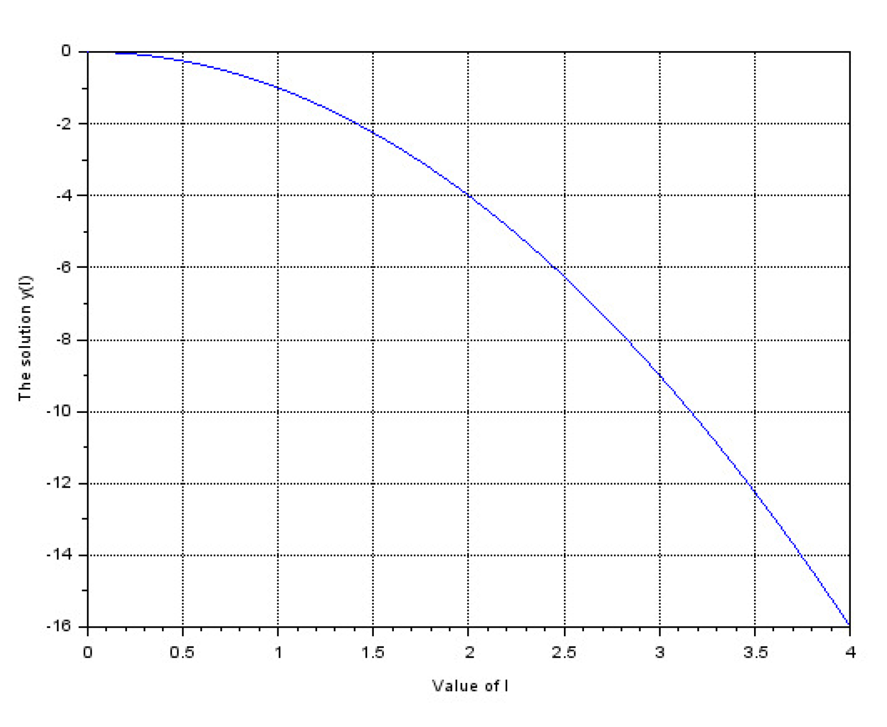
Example 3.

Consider the following GPF Riemann-Liouville initial value problem

$$\begin{array}{c}\hfill \left\{\begin{array}{c}{}_0{D}^{\frac{3}{2},1}y\left(l\right)+\sqrt{l}\left(\frac{4}{\sqrt{\pi }}+\frac{e^{3\sqrt{-y}}}{{(-y)}^{\frac{1}{4}}}\right)=e^{3l},l>0,\hfill \\ \underset{l\to 0^{+}}{lim}{}_0{I}^{\frac{1}{2},1}y\left(l\right)=0.\hfill \end{array}\right.\end{array}$$

(51)

Setting $\alpha =\frac{1}{2}$, $\rho =1$, $a=p\left(l\right)=0$, $q\left(l\right)=\sqrt{l}$, $f\left(y\right)=\frac{4}{\sqrt{\pi }}+\frac{e^{3\sqrt{-y}}}{{(-y)}^{\frac{1}{4}}}$, $g\left(l\right)=e^{3l}$ and $V\left(l\right)=1$. The assumption $\left(H\right)$ is satisfied if $y\left(l\right)>0$. Then,

$${}_{l_1}{I}^{1,\rho }\left(\rho g\left(s\right)V\left(s\right)\right)=\frac{1}{\rho }{\int }_{l_1}^s{e}^{\frac{\rho -1}{\rho }(s-\tau )}\rho g\left(\tau \right)V\left(\tau \right)d\tau ={\int }_{l_1}^s{e}^{3\tau }d\tau =\frac{e^{3s}}{3}-\frac{e^{3l_1}}{3}=\frac{1}{3}\left(e^{3s}-e^{3l_1}\right).$$

By setting $l_1=\frac{1}{3}$ and $l-s={\tau }^2$, it follows that

$$\begin{array}{cc}\hfill & l^{1-\alpha }{\int }_0^l{e}^{\frac{\rho -1}{\rho }(l-s)}{(l-s)}^{\alpha -1}\left[\frac{e^{\frac{\rho -1}{\rho }(s-l_1)}M+{}_{l_1}{I}^{1,\rho }\left(\rho g\left(s\right)V\left(s\right)\right)}{V\left(s\right)}\right]ds\hfill \\ & =l^{\frac{1}{2}}{\int }_0^l{(l-s)}^{-\frac{1}{2}}\left[M+\frac{1}{3}\left(e^{3s}-e\right)\right]ds.\hfill \\ & =l^{\frac{1}{2}}\left[\left(M-\frac{e}{3}\right){\int }_0^l{(l-s)}^{-\frac{1}{2}}ds+\frac{1}{3}{\int }_0^l{(l-s)}^{-\frac{1}{2}}{e}^{3s}ds\right]\hfill \\ & =2l^{\frac{1}{2}}\left[\left(M-\frac{e}{3}\right)\sqrt{l}+\frac{1}{3}{e}^{3l}{\int }_0^{\sqrt{l}}{e}^{-3\tau }d\tau \right].\hfill \end{array}$$

However, the condition (22) does not holds since

$$\begin{array}{cc}\hfill & \underset{l\to \infty }{lim}inf{l}^{1-\alpha }{\int }_0^l{e}^{\frac{\rho -1}{\rho }(l-s)}{(l-s)}^{\alpha -1}\left[\frac{e^{\frac{\rho -1}{\rho }(s-a)}M+{}_{l_1}{I}^{1,\rho }\left(\rho g\left(s\right)V\left(s\right)\right)}{V\left(s\right)}\right]ds\hfill \\ & =\underset{l\to \infty }{lim}inf\left\{2l^{\frac{1}{2}}\left[\left(M-\frac{e}{3}\right)\sqrt{l}+\frac{1}{3}{e}^{3l}{\int }_0^{\sqrt{l}}{e}^{-3\tau }d\tau \right]\right\}\hfill \\ & =\left[\left(M-\frac{e}{3}\right)(+\infty )+(+\infty )\frac{\sqrt{\pi }}{2}\right]=\infty .\hfill \end{array}$$

Using Proposition 1 (ii) with $\alpha =\frac{3}{2}$, $\beta =3$ and $\rho =1$, we get ${{}_{a}D}^{\alpha ,\rho }y\left(l\right)=-\frac{4\sqrt{l}}{\sqrt{\pi }}$, it is easy to verify that $y\left(l\right)=-l^2$ is a nonoscillatory solution of (51). Figure 1 demonstrates the solution $y\left(l\right)=-l^2$.

6. Conclusions

In this paper, the oscillatory behavior of solutions of generalized proportional fractional initial value problem is studied. Forced and damped oscillation results are obtained via GPF operators in the frame of Riemann-Liouville and Caputo settings. The main theorems of this paper improve and generalize some existing oscillation theorems reported in the literature. In particular, for the choice of $\rho =1$, our contributions obtained using GPF operators cover the results discussed in Reference [24] which are obtained via conformable operators. At the end, we presented some numerical examples with particular values of parameters to illustrate the validity of the proposed results. Interestingly, we provided an example demonstrating that the failure of any condition forces the existence of a nonoscillatory solution. This justifies the advantage of our findings.

We believe that the results of this paper are of great importance for the audience of interested researchers. Several types of oscillation conditions could be generalized by considering respective equations within GPF derivatives.

References

1. Miller, K.S.; Ross, B. An Introduction to the Fractional Calculus and Fractional Differential Equations; Wiley: New York, NY, USA, 1993. [Google Scholar]
2. Podlubny, I. Fractional Differential Equations; Academic Press: San Diego, CA, USA, 1999. [Google Scholar]
3. Diethelm, K. The Analysis of Fractional Differential Equations. In Lecture Notes in Mathematics; Springer: Berlin, Germany, 2010. [Google Scholar]
4. Lakshmikantham, V.; Leela, S.; Devi, J.V. Theory of Fractional Dynamic Systems; Cambridge Acadamic Publishers: Cambridge, UK, 2009. [Google Scholar]
5. Kilbas, A.A.; Srivastava, H.M.; Trujillo, J.J. Theory and Application of Fractional Differential Equations; North Holland Mathematics Studies; Elsever: Amsterdam, The Netherlands, 2006; Volume 204. [Google Scholar]
6. Samko, S.G.; Kilbas, A.A.; Marichev, O.L. Fractional Integral and Derivatives: Theory and Applications; Gordon and Breach: Yverdon, Switzerland, 1993. [Google Scholar]
7. Oldham, K.B.; Spanier, J. Fractional Calculus: Theory and Applications, Differentiation and Integration to Arbitrary Order; Academic Press: New York, NY, USA, 1974. [Google Scholar]
8. Hilfer, R. Applications of Fractional Calculus in Physics; Word Scientific: Singapore, 2000. [Google Scholar]
9. Martínez-García, M.; Zhang, Y.; Gordon, T. Memory pattern identification for feedback tracking control in human-machine systems. Hum. Factors 2019. [Google Scholar] [CrossRef] [PubMed] [Green Version]
10. Martínez Garcia, M. Modelling Human-Driver Behaviour Using a Biofidelic Approach. Doctoral Dissertation, University of Lincoln, Lincoln, UK, 2018. [Google Scholar]
11. Khalil, R.; Al Horani, M.; Yousef, A.; Sababheh, M. A new definition of fractional derivative. J. Comput. Appl. Math. 2014, 264, 65–70. [Google Scholar] [CrossRef]
12. Abdeljawad, T. On conformable Calculus. J. Comput. Appl. Math. 2015, 279, 57–66. [Google Scholar] [CrossRef]
13. Anderson, D.R.; Ulness, D.J. Newly defined conformable derivatives. Adv. Dyn. Syst. Appl. 2015, 10, 109–137. [Google Scholar]
14. Caputo, M.; Fabrizio, M. A new definition of fractional derivative without singular kernal. Prog. Frac. Differ. Appl. 2015, 1, 73–85. [Google Scholar]
15. Jarad, F.; Abdeljawad, T.; Alzabut, J. Generalized fractional derivatives generated by a class of local proportional derivatives. Eur. Phys. J. Spec. Top. 2017, 226, 3457–3471. [Google Scholar] [CrossRef]
16. Alzabut, J.; Abdeljawad, T.; Jarad, F.; Sudsutad, W. A Gronwall inequality via the generalized proportional fractional derivative with applications. J. Inequal. Appl. 2019, 2019, 101. [Google Scholar] [CrossRef] [Green Version]
17. Alzabut, J.; Sudsutad, W.; Kayar, Z.; Baghani, H. A new Gronwall-Bellman inequality in a frame of generalized proportional fractional derivative. Mathematics 2019, 7, 747. [Google Scholar] [CrossRef] [Green Version]
18. Shammakh, W.; Alzumi, H.Z. Existence results for nonlinear fractional boundary value problem involving generalized proportional derivative. Adv. Differ. Equ. 2019, 2019, 94. [Google Scholar] [CrossRef] [Green Version]
19. Grace, S.; Agarwal, R.; Wong, P.; Zafer, A. On the oscillation of fractional differential equations. Fract. Calc. Appl. Anal. 2012, 15, 222–231. [Google Scholar] [CrossRef]
20. Chen, D.X.; Qu, P.X.; Lan, Y.H. Forced oscillation of certain fractional differential equations. Adv. Differ. Equ. 2013, 2013, 125. [Google Scholar] [CrossRef] [Green Version]
21. Feng, Q.H.; Meng, F.W. Oscillation of solutions to nonlinear forced fractional differential equations. Electron. J. Differ. Equ. 2013, 2013, 169. [Google Scholar]
22. Pavithra, S.; Muthulaksmi, V. Oscillatory behavior for a class of fractional differential equations. Int. J. Pure Appl. Math. 2017, 115, 93–107. [Google Scholar]
23. Abdalla, B. Oscillation of differential equations in the frame of nonlocal fractional derivatives generated by conformable derivatives. Adv. Differ. Equ. 2018, 2018, 107. [Google Scholar] [CrossRef]
24. Aphithana, A.; Ntouyas, S.K.; Tariboon, J. Forced oscillation of fractional differential equations via conformable erivatives with damping term. Bound. Value Probl. 2019, 2019, 47. [Google Scholar] [CrossRef] [Green Version]
25. Alzabut, J.; Manikandan, S.; Muthulakshmi, V.; Harikrishnan, S. Oscillation criteria for a class of nonlinear conformable fractional damped dynamic equations on time scales. J. Nonlinear Funct. Anal. 2020, 2020, 10. [Google Scholar]
26. Sudsutad, W.; Alzabut, J.; Tearnbucha, C.; Thaiprayoon, C. On the oscillation of differential equations in frame of generalized proportional fractional derivatives. AIMS Math. 2020, 5, 856–871. [Google Scholar] [CrossRef]
27. Anderson, D.R. Second-order self-adjoint differential equations using a proportional-derivative controller. Commun. Appl. Nonlinear Anal. 2017, 24, 17–48. [Google Scholar]
Figure 1. The nonoscillatory behavior of the solution y ( l ) = l 2 .
Mathematics 08 01037 g001