A Geometry-Based Guidance Law to Control Impact Time and Angle under Variable Speeds

Abstract

To provide a feasible solution for a variable speed unmanned aerial vehicle (UAV) to home on a target with impact time and angle constraints, this paper presents a novel geometry-based guidance law composed of trajectory reshaping and tracking. A trajectory generation process using Bezier curves is introduced to satisfy the impact time and angle constraints under time-varying speed. The impact angle is satisfied by driving the UAV along a specified ending line. The impact time is satisfied by controlling the trajectory length, which is realized through adjusting one Bezier curve end point along the ending line. The adjustable range of this end point, along with the maximum trajectory curvature, is analyzed to ensure that the trajectory is flyable. Guidance command is generated using inverse dynamics. Numerical simulations under various scenarios are demonstrated to illustrate the performance and validate the effectiveness of the proposed method.

1. Introduction

1.1. Background

Guidance and control systems, which generate flight commands and execute commands during flights [1], are vital for UAV flights. Traditional guidance laws focus on reducing the distance between a UAV and a target to zero during the flight [2]. However, a zero miss distance may not be enough for all scenarios. To improve performance, extra terminal constraints, such as a minimum of control effort, a specified impact angle and a desired impact time, are imposed. In some cases, the UAVs are expected to approach the target from a specified direction, and an impact angle constraint should be imposed [3]. Impact time control is employed to realize a simultaneous arrival [4], which is needed to gather UAVs into a formation. Due to these important factors, research has been conducted over the past few decades on guidance laws with impact angle and time constraints.

The guidance law proposed in [5] opened a new research area in which both the impact angle and time could be controlled. Henceforth, some valuable contributions have been made in terms of impact time and angle control guidance (ITACG) laws. An ITACG law was developed in [6] by tracking the desired line-of-sight (LOS) rate profile using sliding mode control. In [7], the impact time and angle constraints are satisfied by assuming the guidance command as a polynomial function of time-to-go and properly choosing the coefficients of the guidance command. In [8], the terminal impact time and angle constraints are satisfied by combining the augmented polynomial guidance and adjustable navigation coefficients in terms of a fixed target. In [9], a biased proportional navigation guidance (BPNG)-based ITACG law was proposed, which used feedback controls to eliminate the time-to-go error with a designated heading angle constraint. In [10], time-varying sliding mode (TVSM) control was used to design the ITACG. A specified TVSM with two coefficients is built and the impact constraints are satisfied by adjusting these coefficients. In [11], an ITACG law was developed based on optimal control theory and deviated pure pursuit. Chen and Wang [12] developed an ITACG law by adding a feedback controller to an impact angle control guidance (IACG) law based on optimal control. In [13], a two-stage ITACG was proposed based on nonsingular sliding mode control. The first and second stages are designed to control impact time and impact angle, respectively. In [14], the impact time and angle control problem was solved by shaping the look angle. A polynomial with two coefficients for the impact constraints were obtained, which led to the guidance gain. Based on sliding mode control, an ITACG was developed in [15] by adjusting the gain according to the system state.

However, there are some disadvantages that need to be addressed for the existing ITACG laws. First, because of the implicitness of the flight trajectory, accurately estimating the time-to-go of UAV using guidance laws based on time-domain-control is difficult [5,16]. This difficulty greatly restricts the impact time control and is the reason for the limited number of references related to ITACGs. Some researchers have used linear approximations [6,8,12,17] to estimate the impact time under a small heading angle assumption, which might result in performance degradation under large impact angles [12]. Second, the existing ITACG laws [5,6,7,8,9,11,12,13,14,15] cannot provide an impact time range under given initial conditions, which results in difficulties in ensuring the success of the simultaneous arrival of multiple UAVs. Finally, all the above ITACG laws [5,6,7,8,9,10,11,12,13,14,15] assume that the UAV speed is constant, while in practice, the UAV speed changes over time. Hence, the guidance performance may degrade greatly under variable speed.

Some geometry-based guidance laws offers a perspective for ITACG design. In [18], an IACG law was proposed based on the principle of following a circular arc to the target. In [19], a path planning based guidance law was proposed by combining Dubins’ curves and classical guidance. In [20], Bezier curves were employed to design flight path for parafoil terminal guidance. In [21], a geometry-based IACG was proposed, which uses Bezier curves to design flight path with expected impact angle. From the geometric point of view, the time-to-go of an UAV is the quotient of the remaining trajectory length and UAV velocity. It is easy to obtain with explicit trajectories, even if the speed changes with time. Motivated by this, a novel ITACG law is proposed based on Bezier curves and inverse dynamics [22] in this paper.

1.2. Our Results

In this paper, engine thrust and aerodynamic forces are considered in motion model. The closed-form solution of trajectory length is derived to obtain the impact time effectively. The closed-form solution of the maximum curvature of the trajectory is derived to restrict the required flight maneuverability. The main contributions of this paper are as follows:

(1)

Different from guidance laws with implicit trajectories based on time-domain control, this paper introduces Bezier curves to design trajectories that explicitly satisfy the impact time and angle constraints. The estimation of time-to-go does not involve linear approximations; hence, the precision of impact time control is improved compared with that of [5]. To ensure that the UAV is capable of flying along the obtained trajectory, an acceleration limit is considered by restricting the maximum curvature of the trajectory. Some other ITACG laws such as [6] may not fully consider this factor.

(2)

The time-varying speed is considered in the guidance law design, while the existing ITACG laws, such as those in [5,6,7,8,9,10,11,12,13,14,15], did not consider this practical factor that greatly affects the actual flight. Moreover, compared with other ITACG laws, the proposed law provides an impact time range according to the given conditions before launch, which enhances cooperation among UAVs by controlling the impact time.

The paper is organized as follows: Section 2 formulates the guidance problem. In Section 3, an ITACG law is presented based on quadratic Bezier curves and inverse dynamics. In Section 4, simulations are performed to demonstrate the effectiveness and performance of the guidance law. Section 5 provides the conclusions.

2. Guidance Problem Statement

For a UAV, the guidance system generates the acceleration command according to the flight mission and feeds it to the flight control system. Then, the flight control system usually uses actuators, such as elevators and rudders, to execute the commands by adjusting the lift and lateral forces in the pitch and yaw planes of the UAV [23]. Therefore, three-dimensional motion can usually be decoupled into two mutually orthogonal planes corresponding to the pitch and yaw planes of the flight control system [24]. Consequently, many studies related to guidance laws were conducted in two dimensions [5,6,11,12,17].

Assume that the UAV needs to arrive at the target position as shown in Figure 1. The UAV and target position are denoted by I and T, respectively. The UAV travels at a time-varying speed $V\left(t\right)$, with a maximum acceleration limit $a_{max}$. Both the target and the UAV are assumed to be mass points. The coordinates of the UAV and the target in the geographic frame $X-O-Y$ are ${(x_m,y_m)}^T$ and ${(x_t,y_t)}^T$ respectively. a is the UAV’s lateral acceleration command perpendicular to the velocity vector. The UAV’s heading angle and LOS angle are represented by $\theta$ and $\lambda$, respectively. The desired impact angle is denoted by ${\theta }_f$. The angle between the LOS and velocity vector is denoted by $\sigma$. A positive angle is one of anticlockwise rotation.

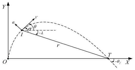
Figure 1. Guidance geometry between missile I and target T, along with variable definitions of $\sigma$, $\theta$ and $\lambda$.

In the derivation of the UAV’s equations of motion, gravity is neglected. The drag model is composed of two types of drag, namely parasitic (zero-lift) drag and induced drag. The parasitic drag is borrowed from [25,26]. The variation of the UAV’s speed due to engine thrust T and aerodynamic drag D is expressed as follows

$$\begin{array}{c}{\displaystyle \frac{dV}{dt}}={\displaystyle \frac{1}{m}}(T-D)\end{array}$$

(1)

The engine thrust T, aerodynamic drag D and UAV’s mass m are expressed as

$$T\left(t\right)=\left\{\begin{array}{c}{T}_{en},t\le t_{en}\hfill \\ 0,t>t_{en}\hfill \end{array}\right.$$

(2)

$$D\left(t\right)=\frac{1}{2}\rho V{\left(t\right)}^{2}S{C}_D+k_D{a}^2$$

(3)

$$m\left(t\right)=\left\{\begin{array}{c}{m}_0-{\int }_0^t\mu dt,t\le t_{en}\hfill \\ m_0-m_{fu},t>t_{en}\hfill \end{array}\right.$$

(4)

where S and $\rho$ are the UAV’s cross-sectional area and air density, respectively. $C_D$ is the parasitic drag coefficient, and its relationship with the UAV speed V is presented in Figure 2. $k_D$ is the induced drag coefficient, which is set to 0.05. $T_{en}$, $\mu$, $m_{fu}$ and $t_{en}$ are the thrust, fuel consumption rate, fuel mass and maximum working time of the UAV engine, respectively.

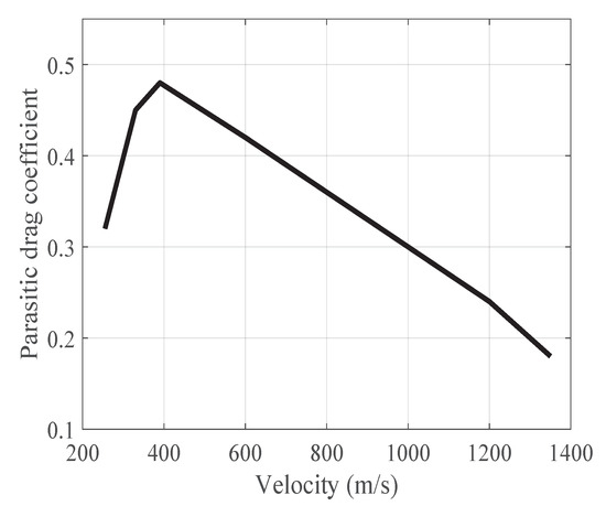
Figure 2. Profile of the parasitic drag coefficient of UAV with respect to speed (used for calculating aerodynamic drag).

Assuming the autopilot dynamics are fast enough to be neglected, the flight kinematics of the UAV is represented by

$$\begin{array}{c}{\displaystyle \frac{d{x}_m}{dt}}=Vcos\theta \\ {\displaystyle \frac{d{y}_m}{dt}}=Vsin\theta \\ {\displaystyle \frac{d\theta }{dt}}={\displaystyle \frac{a}{V}}\\ \left|a\right|\le a_{max}\end{array}$$

(5)

The range variation and LOS rate is governed by

$$\dot{r}=-Vcos\sigma$$

(6)

$$\dot{\lambda }=\frac{-Vsin\sigma }{r}$$

(7)

The guidance goal is to generate acceleration command a for the UAV such that it can arrive at target T at a desired time with a specified impact angle:

$$\begin{array}{c}\underset{t\to t_f}{lim}{x}_m\to x_T,\underset{t\to t_f}{lim}{y}_m\to y_T,\underset{t\to t_f}{lim}\theta \to -{\theta }_f,\end{array}$$

(8)

where $t_f$ is the desired impact time. For simplicity, the origin of the reference frame is set at the UAV launch point, while the related positive X axis is set to pass through the target position. Thus, the UAV positions at launch time and impact time are ${(0,0)}^T$ and ${(x_t,0)}^T$, respectively. Notably, such a reference frame is a local frame with respect to a UAV. If the UAVs are launched from different positions, the relevant local frames should be established as described in Section 4.3.

3. Guidance Law Design

In this section, the ITACG law based on trajectory reshaping and inverse dynamics is developed. First, a trajectory generation process based on Bezier curves is introduced to satisfy the impact time and angle constraints. To ensure that this trajectory is flyable, the trajectory curvature is constrained, which further restricts the position of the phase switching point. Then, the impact time range can be obtained based on this position range. Inverse dynamics are used to design guidance law. The block diagram of guidance and control is depicted in Figure 3.

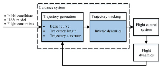
Figure 3. Guidance and control block diagram.

3.1. Trajectory Generation

The trajectory of the UAV near impact can be regarded as a straight line. Therefore, if this ending line forms an angle equal to ${\theta }_f$, the impact angle can be achieved. On this basis, the guidance law just needs to guide the UAV from the initial velocity vector to the ending line and then keep it travelling along this line, corresponding to the initial phase and the terminal phase, respectively. Figure 4 illustrates the two-phase guidance process. The point connecting the trajectories of the two phases, denoted by P, is called the phase switching point.

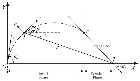
Figure 4. Two guidance phases of the proposed ITACG, the initial phase aims to enter the ending line smoothly at phase switching point P while the terminal phase aims to fly along the ending line.

According to the desired target position and impact angle, the ending line can be obtained as

$$y=tan\left({\theta }_f\right)(x-x_t)$$

(9)

Likewise, the starting line, which coincides with the initial velocity vector, is represented as

$$y=tan\left({\theta }_0\right)x$$

(10)

where ${\theta }_0$ is the UAV’s heading angle at launch. Moreover, to avoid an infinite acceleration command, the entire trajectory must be smooth (first-order continuous). Hence, the trajectory of the initial phase needs to be tangent to both the starting and ending lines. Therefore, we introduce the Bezier curve to fulfill the task, which is mathematically defined as

$$B(\tau )=\sum _{i=0}^n{b}_{i,n}\left(\tau \right)P_{i}0\le \tau \le 1$$

(11)

where $b_{i,n}\left(\tau \right)$ are the Bernstein basis polynomials of degree n, which can be represented as $b_{i,n}\left(\tau \right)=\frac{n!}{i!(n-i)!}{\tau }^i{(1-\tau )}^{n-i}$. $\tau$ is the curve parameter taking values between 0 and 1. $P_i$ are the control and end points.

Here, we choose the Bezier curve with a degree of two, and this quadratic Bezier curve is specified by end points $E_1$, $E_2$ and control point C. The curve trajectory is constructed by setting $E_1$ at the launch point O, $E_2$ at the phase switching point P and C at the intersection point Q of the starting and ending lines, as shown in Figure 5. Note that points $E_1$ and $E_2$ are fixed under given initial conditions, and point $E_2$ is the only tunable point along the ending line.

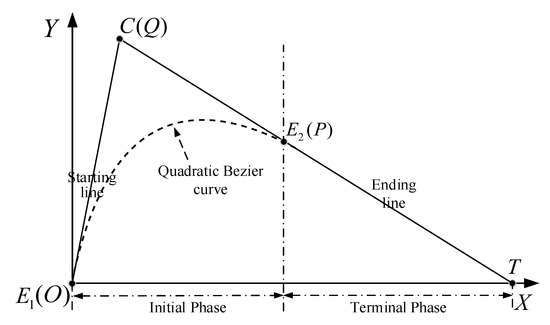
Figure 5. Two-phase trajectory of the proposed ITACG. The initial-phase trajectory (a quadratic Bezier curve) and terminal-phase trajectory (a straight line) are tangent to each other.

Substituting the points and $n=2$ into Equation (11) leads to

$$B(\tau )=(1-\tau {)}^2{E}_1+2(1-\tau )\tau C+{\tau }^2{E}_2$$

(12)

The properties of the quadratic Bezier curve are listed as follows, and the corresponding proofs, which are omitted here, can be found in [27]. Notably, Bezier curve or surfaces are specific cases of parametric algebraic varieties, which are often studied with their semigroup ring. Other related mathematical properties can be referred to [28,29]

• Property 1: Given a quadratic Bezier curve $B\left(\tau \right)$ with end points $E_1$ and $E_2$ and control point C, it can be derived that $B\left(0\right)=E_1$ and $B\left(1\right)=E_2$.
• Property 2: Given a quadratic Bezier curve $B\left(\tau \right)$ with end points $E_1$ and $E_2$ and control point C, it can be derived that line $E_{1}C$ is tangent to this Bezier curve at point $E_1$; likewise, line $E_{2}C$ is tangent to the Bezier curve at point $E_2$.

According to Properties 1 and 2, the quadratic Bezier curve segment in Figure 5 is tangent to the ending line, and the entire trajectory meets the design requirement of first-order continuity. Since the impact time is essentially determined by the quotient of the trajectory length and the UAV speed, we can control the impact time by adjusting the trajectory length. Therefore, we need to derive the relationship between the trajectory length and the only tunable point $E_2$ to satisfy the impact time constraint.

The derivative of Equation (12) can be obtained as

$$\begin{array}{c}{\displaystyle \frac{dx}{d\tau }}=-2(1-\tau )x_{E_1}+2(1-2\tau )x_Q+2\tau x_{E_2}\\ {\displaystyle \frac{dy}{d\tau }}=-2(1-\tau )y_{E_1}+2(1-2\tau )y_Q+2\tau y_{E_2}\end{array}$$

(13)

where $(x_{E_1},y_{E_1})$, $(x_Q,y_Q)$ and $(x_{E_2},y_{E_2})$ are the coordinates of points $E_1$, Q and $E_2$ respectively. The relationship between the entire trajectory length and point $E_2$ can be expressed as

$$L\left(x_{E_2}\right)={\int }_0^1\sqrt{{\left(\frac{dx}{d\tau }\right)}^2+{\left(\frac{dy}{d\tau }\right)}^2}d\tau +\frac{x_t-x_{E_2}}{cos\left({\theta }_f\right)}$$

(14)

To obtain the desired impact time effectively, a closed-form solution of trajectory length needs to be derived. Equations (12) and (14) can be rewritten as

$$B\left(\tau \right)=J{\tau }^2+2K\tau$$

(15)

$$L={\int }_0^{1}2\sqrt{{\left|J\right|}^2{\tau }^2+2\left(J·K\right)\tau +{\left|K\right|}^2}d\tau +\frac{x_t-x_{E_2}}{cos\left({\theta }_f\right)}$$

(16)

where $J=E_1-2Q+E_2$ and $K=Q-E_1$. Setting $D=\left(J·K\right)/{\left|J\right|}^2$ and $E={\left|K\right|}^2/{\left|J\right|}^2$, we have

$$L=2\left|J\right|{\int }_0^1\sqrt{{\tau }^2+2D\tau +E}d\tau +\frac{x_t-x_{E_2}}{cos\left({\theta }_f\right)}$$

(17)

Substituting $u=\tau +D$ into Equation (17) leads to

$$L=2\left|J\right|{\int }_D^{1+D}\sqrt{u^2+U}du+\frac{x_t-x_{E_2}}{cos\left({\theta }_f\right)}=\left|J\right|\left[N(1+D)-N\left(D\right)\right]+\frac{x_t-x_{E_2}}{cos\left({\theta }_f\right)}$$

(18)

where $U=E-D^2$ and $N\left(\mathrm{u}\right)=\mathrm{u}\sqrt{u^2+U}+Ulog(u+\sqrt{u^2+U})$. Substituting $D=\left(J·K\right)/{\left|J\right|}^2$, $E={\left|K\right|}^2/{\left|J\right|}^2$ and $W=J+K$ into Equation (18), we have

$$L=\frac{\left|W\right|\left(J·W\right)-\left|K\right|\left(J·K\right)}{{\left|J\right|}^2}+(\frac{{\left|K\right|}^2}{\left|J\right|}-\frac{{\left(J·K\right)}^2}{{\left|J\right|}^3})log\frac{\left|J\right|\left|W\right|+J·W}{\left|J\right|\left|K\right|+J·K}$$

(19)

However, due to the time-varying speed, the obtained trajectory is not an interception trajectory for an arbitrary impact time. For $t_f$ to be the interception time, the following equation must be satisfied:

$$\beta (t_f,x_{E_2})={\int }_0^{t_f}{\int }_0^t\dot{V}\left(\sigma \right)d\sigma dt-L=0$$

(20)

The above equation states that the distance traveled by the UAV along the given trajectory from $t=0$ to $t_f$ is equal to the length of the designed trajectory, which implies that interception occurs at $t_f$.

3.2. Trajectory Curvature Analysis

Because the acceleration command is essentially determined by the trajectory curvature, the maximum curvature must be constrained according to the acceleration limit $a_{max}$. Since the trajectory of the terminal phase is a straight line, we need to investigate only the curvature of the initial phase trajectory. According to Equation (13), we have    

$$\begin{array}{c}{B}^{\prime }\left(\tau \right)=-2(1-\tau )E_1+2(1-2\tau )C+2\tau E_2\\ B^{\prime \prime }\left(\tau \right)=2E_1-4C+2E_2\\ B^{\prime }\left(0\right)=-2E_1+2C\\ B^{\prime }\left(1\right)=-2c+2E_2\end{array}$$

(21)

The signed curvature $k\left(\tau \right)$ of quadratic Bezier curve [30] can be expressed as

$$k\left(\tau \right)=\frac{B^{\prime }\left(\tau \right)\times B^{\prime \prime }\left(\tau \right)}{{\left|B^{\prime }\left(\tau \right)\right|}^3}$$

(22)

Substituting the coordinates of C and $E_2$ into Equation (22), we obtain

$$k\left(\tau \right)=\frac{-4|E_1{E}_2|l}{|B^{\prime }\left(\tau \right){|}^3}$$

(23)

where l is the distance from point C to line $E_1{E}_2$. Differentiating Equation (23) gives

$$k^{\prime }\left(\tau \right)=\frac{12|E_1{E}_2|l}{|B^{\prime }\left(\tau \right){|}^4}{\left|B^{\prime }\left(\tau \right)\right|}^{\prime }$$

(24)

Thus, $k\left(\tau \right)$ is monotone if and only if

$$\forall \tau \in (0,1),|B^{\prime }{\left(\tau \right)|}^{\prime }\ne 0$$

(25)

Proposition 1.

Given a quadratic Bezier curve $B\left(\tau \right)$ with end points $E_1$ and $E_2$ and control point C, the midpoint of $E_1{E}_2$ is denoted by M. It can be shown that, if $\angle E_{1}CM$ or $\angle MC{E}_2$ is equal to or larger than $\pi /2$, then $B\left(\tau \right)$ has a monotone curvature; otherwise, $B\left(\tau \right)$ has a nonmonotone curvature.

Proof. 

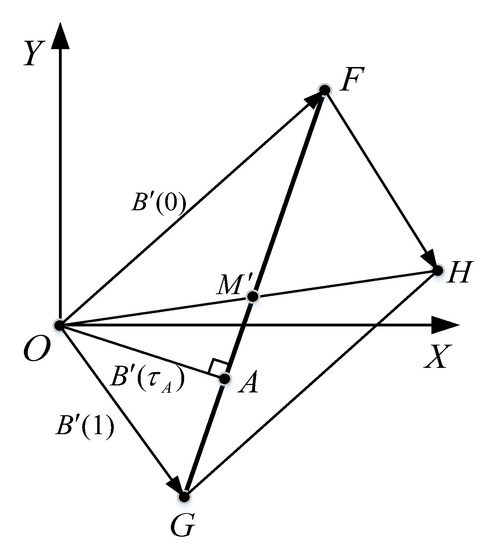
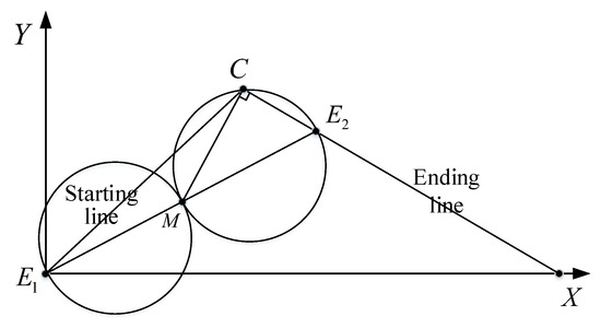
It can be observed from Equation (21) that $B^{\prime }\left(\tau \right)$ is a segment with two end points $F=B^{\prime }\left(0\right)$ and $G=B^{\prime }\left(1\right)$, as shown in Figure 6. First, the parallelogram $OFHG$ with triangle $OFG$ is constructed, and $M^{\prime }$ is the midpoint of segment $OH$. According to Equation (21), $\overrightarrow{OF}=B^{\prime }\left(0\right)=2\overrightarrow{E_{1}C}$ and $\overrightarrow{FH}=\overrightarrow{OG}=B^{\prime }\left(1\right)=2\overrightarrow{C{E}_2}$. Therefore, triangle $OFH$ is similar to triangle $E_{1}C{E}_2$, which leads to $\angle OFG=\angle E_{1}CM$ and $\angle OGF=\angle MC{E}_2$. Assume there is a value ${\tau }_A\in (0,1)$ with $|B^{\prime }\left({\tau }_A\right){|}^{\prime }=0$. Then, $B^{\prime }\left({\tau }_A\right)$ is equal to the vector $\overrightarrow{OA}$, which is perpendicular to $FG$. Thus, the curvature of the quadratic Bezier curve is monotone if and only if A lies outside segment $FG$. Such a condition can be met when $\angle OFG=\angle E_{1}CM\ge \pi /2$ or $\angle OGF=\angle MC{E}_2\ge \pi /2$. Figure 7 shows a critical condition of monotone curvature, where $\angle MC{E}_2=\pi /2$. □

Figure 6. Sketch of the first derivative of the quadratic Bezier curve $B\left(\tau \right)$, showing the relationships among $B^{\prime }\left(0\right)$, $B^{\prime }\left(1\right)$ and $B^{\prime }\left({\tau }_A\right)$.

Figure 7. A critical condition of monotone curvature, in which $\angle OGF=\angle MC{E}_2=\pi /2$ and corresponds to the condition that point A lies at the end point of segment $FG$ in Figure 6.

Proposition 2.

The maximum absolute curvature of the trajectory can be expressed as

$$|k{\left(\tau \right)}_{max}|=\left\{\begin{array}{c}max\left\{\left|k\left(0\right)\right|,\left|k\left(1\right)\right|\right\},\angle E_{1}CM>\pi /2\mathrm{or}\angle MC{E}_2>\pi /2\hfill \\ {\displaystyle \frac{min\left\{\left|k\right(0\left)\right|,\left|k\right(1\left)\right|\right\}}{min\left\{{sin}^3\angle E_{1}CM,{sin}^3\angle MC{E}_2\right\}}},\mathrm{otherwise}\hfill \end{array}\right.$$

(26)

Proof. 

The curvature variation can be divided into two cases: a monotone curvature and a nonmonotone curvature. For a monotone curvature, the maximum value of $\left|k\right(\tau \left)\right|$ is obtained as

$${\left|k\left(\tau \right)\right|}_{max}=max\left\{\left|k\left(0\right)\right|,\left|k\left(1\right)\right|\right\}$$

(27)

□

Specifically, if $\angle E_{1}CM\ge \pi /2$, then ${\left|k\left(\tau \right)\right|}_{max}=\left|k\left(0\right)\right|$ and the maximum value of $\left|k\right(\tau \left)\right|$ is achieved at launch. Likewise, if $\angle MC{E}_2\ge \pi /2$, then ${\left|k\left(\tau \right)\right|}_{max}=\left|k\left(1\right)\right|$ and the maximum value of $\left|k\right(\tau \left)\right|$ is achieved at impact.

When the curvature is nonmonotone, $\left|k\right(\tau \left)\right|$ reaches its maximum value at $\tau ={\tau }_A$ (where $|B^{\prime }\left({\tau }_A\right){|}^{\prime }=0$) and its minimum value at either $\tau =0$ or $\tau =1$. Hence, the ratio of the maximum value to minimum one of $\left|k\right(\tau \left)\right|$ is

$${\displaystyle \frac{|k\left(\tau \right){|}_{max}}{|k\left(\tau \right){|}_{min}}}={\displaystyle \frac{\left|k\right({\tau }_A\left)\right|}{min\left\{\left|k\right(0\left)\right|,\left|k\right(1\left)\right|\right\}}}$$

(28)

Substituting Equation (23) into Equation (28) leads to

$${\displaystyle \frac{|k\left(\tau \right){|}_{max}}{|k\left(\tau \right){|}_{min}}}={\displaystyle \frac{max\left\{\right|B^{\prime }\left(0\right){|}^3,|B^{\prime }\left(1\right){|}^3\}}{|B^{\prime }\left({\tau }_A\right){|}^3}}={\displaystyle \frac{max\left\{\right|OF{|}^3,|OG{|}^3\}}{|OA{|}^3}}$$

(29)

According to the proof of Proposition 1, the following equations can be obtained

$$\begin{array}{c}{\displaystyle \frac{\left|OA\right|}{\left|OF\right|}}=sin\angle OFG=sin\angle E_{1}CM\hfill \\ {\displaystyle \frac{\left|OA\right|}{\left|OG\right|}}=sin\angle OGF=sin\angle MC{E}_2\hfill \end{array}$$

(30)

Finally, substituting Equation (30) into Equation (29) leads to

$$\frac{|k\left(\tau \right){|}_{max}}{|k\left(\tau \right){|}_{min}}=\frac{1}{min\{{sin}^3\angle E_{1}CM,{sin}^3\angle MC{E}_2\}}$$

(31)

3.3. Impact Time Analysis

With fixed points $E_1$ and C, the impact time can be adjusted by tuning the position of $E_2$ along the ending line. Moreover, to ensure that the required acceleration for traveling along the trajectory is within the UAV’s capability, the position range of $E_2$ is constrained by the acceleration limit $a_{max}$.

It can be observed from Equation (26) that the maximum absolute curvature is related to $\left|k\right(0\left)\right|$ and $\left|k\right(1\left)\right|$, regardless of whether the curvature is monotone. Differentiating $\left|k\right(0\left)\right|$ and $\left|k\right(1\left)\right|$ with respect to $x_{E_2}$ leads to

$$\begin{array}{c}\frac{d\left|k\right(0\left)\right|}{d{x}_{E_2}}=\frac{y_{E_1}-y_Q}{2{\left[{(x_Q-x_{E_1})}^2+{(y_Q-y_{E_1})}^2\right]}^{3/2}}\\ \\ \frac{d\left|k\right(1\left)\right|}{d{x}_{E_2}}=\frac{16\left[{(x_{E_2}-x_Q)}^2+{(y_{E_2}-y_Q)}^2\right](y_{E_1}-y_Q)+48(x_{E_2}-x_Q)\left[x_Q(y_{E_1}-y_{E_2})+x_{E_1}(y_{E_2}-y_Q)+x_{E_2}(y_Q-y_{E_1})\right]}{32{\left[{(x_{E_2}-x_Q)}^2+{(y_{E_2}-y_Q)}^2\right]}^{\frac{5}{2}}}\end{array}$$

(32)

We can find that $\frac{d\left|k\right(1\left)\right|}{d{x}_{E_2}}$ approaches infinity when $x_{E_2}$ approaches $x_Q$. Therefore, there must be a minimum distance between points $E_2$ and Q to ensure that the trajectory is flyable, and this minimum distance further affects the impact time range denoted by $[t_{fmin},t_{fmax}]$. In summary, $[t_{fmin},t_{fmax}]$ is determined by the initial conditions, including the initial range $x_t$, the initial heading angle ${\theta }_0$, the impact angle ${\theta }_f$ and phase switching point $E_2$, among which only $E_2$ is tunable and can be used to control the impact time.

Based on the previous discussion, the relationship between point $E_2$ and impact time $t_f$ can be expressed as

$$\begin{array}{c}\beta (t_f,x_{E_2})=0\hfill \\ s.t.y_{E_2}=tan(-{\theta }_f)(x_{E_2}-x_t)\hfill \\ |k\left(\tau \right){|}_{max}\le a_{max}/V^2,\tau \in [0,1]\hfill \\ x_{E_2}\in (x_Q,x_{\mathrm{t}}]\hfill \end{array}$$

(33)

Thus, point $E_2$ can be obtained using sequential quadratic programming (SQP) method, which considers trajectory length and curvature constraints. To obtain the impact time range, the following objective function is employed.

$$\begin{array}{c}min\mathrm{or}max{t}_f\hfill \\ s.t.x_{E_2}\in (x_Q,x_{\mathrm{t}}]\hfill \\ \beta (t_f,x_{E_2})=0\hfill \\ y_{E_2}=tan(-{\theta }_f)(x_{E_2}-x_t)\hfill \\ |k\left(\tau \right){|}_{max}\le a_{max}/V^2,\tau \in [0,1]\hfill \end{array}$$

(34)

The generation process of the trajectory that satisfies the impact time and angle constraints is given in Algorithm 1.

Algorithm 1 Trajectory generation process to satisfy the impact time and angle constraints

1: According to the initial condition and impact angle constraint, compute the starting and ending lines using Equations (9) and (10). 2: According to the impact time constraint, use SQP method to find the desired phase switching point along the ending line with the objective function (34). 3: Calculate the trajectory using Equation (12) based on the obtained phase switching point.

3.4. Guidance Law Design Using Inverse Dynamics

Since the previous section provides a shape-dependent trajectory, and the guidance command is usually time-dependent. The time-dependent motion Equation (5) needs to be transformed into shape-dependent motion equations [21,22] as follows

$$\begin{array}{c}{\displaystyle \frac{dy}{dx}}=tan\theta \\ {\displaystyle \frac{d\theta }{dx}}={\displaystyle \frac{a}{V^{2}cos\theta }}\end{array}$$

(35)

According to the first formula of Equation (35), the current heading angle can be obtained as

$$\theta =arctan\left({\displaystyle \frac{dy}{dx}}\right)$$

(36)

Differentiating Equation (36) with respect to x leads to

$${\displaystyle \frac{d\theta }{dx}}={\displaystyle \frac{1}{1+{\left({\displaystyle \frac{dy}{dx}}\right)}^2}}·{\displaystyle \frac{d^{2}y}{d{x}^2}}={\displaystyle \frac{d^{2}y}{d{x}^2}}{cos}^2\theta$$

(37)

Substituting the above equation into the second formula of Equation (35) leads to

$$a=\frac{d^{2}y}{d{x}^2}{V}^2{cos}^3\theta$$

(38)

Differentiating Equation (13) with respect to $\tau$, we have

$$\begin{array}{c}{\displaystyle \frac{d^{2}x}{d{\tau }^2}}=2x_{E_1}-4x_Q+2x_{E_2}\\ {\displaystyle \frac{d^{2}y}{d{\tau }^2}}=2y_{E_1}-4y_Q+2y_{E_2}\end{array}$$

(39)

Thus, $(d^{2}y/d{x}^2)$ can be obtained as

$${\displaystyle \frac{d^{2}y}{d{x}^2}}={\left({\displaystyle \frac{dy/d\tau }{dx/d\tau }}\right)}^{\prime }={\displaystyle \frac{{\displaystyle \frac{d^{2}y}{d{\tau }^2}}·{\displaystyle \frac{dx}{d\tau }}-{\displaystyle \frac{dy}{d\tau }}·{\displaystyle \frac{d^{2}x}{d{\tau }^2}}}{{\left({\displaystyle \frac{dx}{d\tau }}\right)}^2}}$$

(40)

The guidance command is obtain by substituting Equations (13), (39) and (40) into Equation (38).

$$a=\frac{V^2{cos}^3\theta \left[x_Q(-y_{E_1}+y_{E_2})+x{}_{E_2}(y_{E_1}-y_Q)+x_{E_1}(-y_{E_2}+y_Q)\right]}{{[(-1+\tau )x_{E_1}+\tau (x_{E_2}-2x_Q)+x_Q]}^2}$$

(41)

It can be seen that the guidance command is a function of coordinates of points $E_1$, Q and $E_2$ and curve parameter $\tau$. A mapping from $\tau$ to t is needed to generate guidance command with respect to time t, along with time-index waypoints of the reference trajectory (see Appendix A).

The UAV’s flight may be affected by the presence of disturbances. Therefore, a correction process is needed to update the trajectory and guidance command, as described in Figure 8. When the tracking error, i.e., the distance between the UAV position and the time-index reference waypoint, is greater than $d_{err}$, the Bezier curve is updated and reshaped according to the UAV’s current state $(x_m,y_m,\theta )$, target position $(x_T,0)$, impact time constraint $t_f$ and impact angle constraint ${\theta }_f$ using Algorithm 1.

Figure 8. Trajectory update procedure.

4. Simulation and Results

In this section, simulations are performed to demonstrate the performance of the proposed ITACG law. The simulation results of the ITACG law in [5], which is often used as a benchmark [10,12], are presented for comparison. The UAVs using the proposed guidance law and the ITACG law in [5] are denoted by UAV 1 and 2 in the comparative analysis, respectively.

UAV engine thrust $T_{en}=$ 10,000 N, maximum working time of the engine $t_{en}=10$ s, fuel consumption rate $\mu =10$ kg/s, fuel mass $m_{fu}=100$ kg, and maximum lateral acceleration limit $a_{max}=200$$\mathrm{m}/{\mathrm{s}}^2$. The target is positioned at (10,000,0)${}^T$ m. The simulation time step is 0.01 s.

4.1. Case 1: Single Flight under Constant Speed

This subsection shows the simulation results with constant UAV speed $V=300$ m/s, initial heading angle ${\theta }_0={60}^{\circ }$ and desired impact angle ${\theta }_f=-{65}^{\circ }$. The UAVs are launched at $t=0$ s. The impact time range calculated using Equation (34) is $[48.27,63.21]$ s. To minimize the time of intercept, the desired impact time is set to $t_f=48.27$ s.

The trajectories are shown in Figure 9a, which shows that both UAVs arrive at the target accurately. However, according to the relative range variation given in Figure 9b, UAV 2 arrives at the target a little late, at $t=48.78$ s, while UAV 1 arrives at the target punctually, at $t=48.27$ s. This result reveals that the linear approximation in [5] is not accurate enough for a large impact angle and results in time errors, which is in line with [12]. Figure 9c shows the acceleration profile. The energy cost function is defined as the integral of the square of the acceleration command, i.e., $J=\frac{1}{2}{\int }_0^{t_f}{a}^2\left(t\right)dt$. Then the energy cost of both guidance laws are

$$J_{proposed}=7045.0,J_{ITACG\left[5\right]}=8667.6$$

(42)

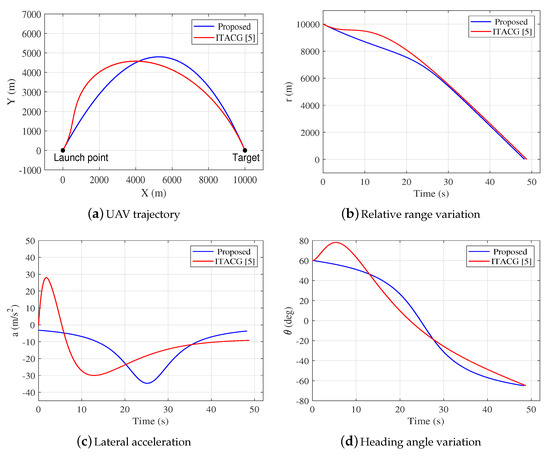
Figure 9. Simulation results of Case 1.

From Equation (42), it can be revealed that the proposed guidance law requires 23.03% less energy than the one in [5]. Moreover, it can be observed from Figure 9a,b that UAV 2 takes an S-shaped detour to satisfy the impact time constraint, which will results in a greater control effort and a reduction of UAV speed in practice. In contrast, UAV 1 adjusts the impact time through a smoother detour, which helps reduce control effort and fuel in practice. This because the UAV 1 has a global planning for the flight before launch while UAV 2 doesn’t. The comparative result is in good agreement with Equation (42). The heading angle variation is presented in Figure 9d, showing that both guidance laws satisfy the impact angle constraint.

4.2. Case 2: Single Flight under Time-Varying Speed

This subsection shows the simulation results under the same conditions as Case 1 except that the UAV speed varies with time, as given in Equations (1)–(4). The impact time range calculated using Equation (34) is $[27.9,33.34]$ s. To minimize the time of intercept, the desired impact time is set to $t_f=27.59$ s.

It can be observed from Figure 10a,b that both UAVs arrive at the target accurately with the desired impact angle, and the impacts occur at $t=27.60$ and $33.98$ s for UAVs 1 and 2, respectively. The variable speed has almost no effect on the performance of the proposed guidance law, while the performance of the guidance law in [5] degrades greatly with variable speed in terms of impact time control. Figure 10c shows the acceleration profile. It can be seen that oscillation occurs in the acceleration history of UAV 2 due to varying speed, whilst the acceleration history of UAV 1 appears to be stable. Figure 10d shows the heading angle variation, which implies both guidance laws achieve the desired impact angle.

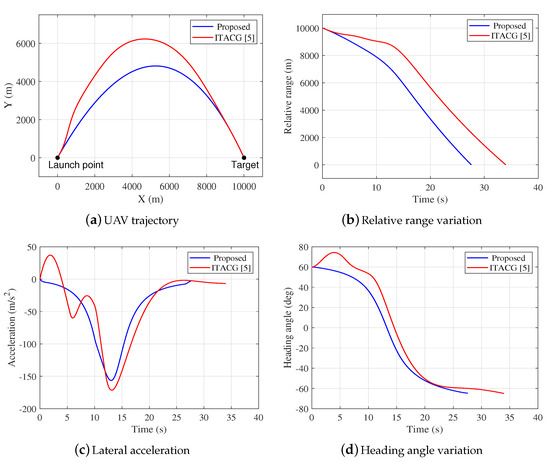
Figure 10. Simulation results of Case 2.

4.3. Case 3: Simultaneous Arrival under Time-Varying Speed

In this subsection, the simultaneous arrival of three variable speed UAVs launched from two different positions is simulated. Three UAVs, $I_1$, $I_2$ and $I_3$, with the initial conditions shown in Table 1, are launched at $t=0$, 1 and 3 s, respectively.

Table 1. Initial conditions of Case 3 in the geographic frame.

UAV	Launch Position (m)	Initial Heading Angle (deg)	Desired Impact Angle (deg)	Target Position (m)
$I_1$	(0,0)	45	−45	(10,000,0)
$I_2$	(0,0)	45	−45	(10,000,0)
$I_3$	(4000,−7000)	90	0	(10,000,0)

Note that the initial conditions are defined in the geographic frame, and need to be transformed to those in the local frames. Such a scenario is shown in Figure 11, where the geographic frame and local frame of the ith UAV are denoted by $O_E-X_E-Y_E-Z_E$ and $O_i-X_i-Y_i-Z_i$, respectively. The origins of the local frames, denoted by $O_i$, are set at the corresponding launch positions, while the related positive $X_i$ axes are set to pass through target position T. Equation (43) gives the coordinate transformation from the geographic frame to the local frame.

$$\left[\begin{array}{c}{x}_i\hfill \\ y_i\hfill \end{array}\right]=\left[\begin{array}{cc}cos{\theta }_{L_i}& -sin{\theta }_{L_i}\\ sin{\theta }_{L_i}& cos{\theta }_{L_i}\end{array}\right]\left[\begin{array}{c}{x}_E-x_{O_i}\hfill \\ y_E-y_{O_i}\hfill \end{array}\right]$$

(43)

where ${(x_i,y_i)}^T$ and ${(x_E,y_E)}^T$ are the coordinates in the local frames and geographic frame, respectively. ${(x_{O_i},y_{O_i})}^T$ are the coordinates of point $O_i$ in the geographic frame. ${\theta }_{L_i}$ is the angle between vector $\overrightarrow{O_{i}T}$ and the positive $X_E$ axis.

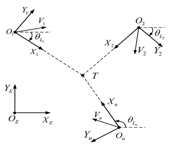
Figure 11. Geographic frame and local frames.

The initial conditions of Case 3 in local frames are given in Table 2.

Table 2. Initial conditions of Case 3 in the corresponding local frames.

UAV	Launch Position (m)	Initial Heading Angle (deg)	Desired Impact Angle (deg)	Target Position (m)
$I_1$	(0,0)	45	−45	(10,000,0)
$I_2$	(0,0)	45	−45	(10,000,0)
$I_3$	(0,0)	40.60	−49.40	(9219.5,0)

The impact time ranges are given in Table 3. To minimize the time of intercept, the desired salvo attack time is set to $t_f=21.67s$.

Table 3. Impact time ranges of Case 3.

UAV	${\mathit{t}}_{\mathit{f},\mathit{min}}$(s)	${\mathit{t}}_{\mathit{f},\mathit{max}}$(s)
$I_1$	20.51	24.01
$I_2$	21.51	25.01
$I_3$	21.67	24.43
Intersection	$\mathsf{\Omega }=[21.46,22.82]$

The trajectories of the three UAVs are shown in Figure 12a, and all the UAVs arrive at the target position accurately. It can be observed that compared with $I_1$, $I_2$ takes a shortcut to compensate for the launch time lag. Figure 12b shows the variation of the relative ranges between the UAVs and the target, showing that the impacts occur at $t=21.65$ s, $21.67$ s and $21.66$ s for $I_1$, $I_2$ and $I_3$, respectively. The acceleration and heading angle variation are given in Figure 12c,d, respectively. It can be seen that the heading errors decrease monotonically and all three UAVs achieve the desired impact angles. The simulation results demonstrate that the proposed geometry-based guidance law can control the impact time and angle of UAVs under variable speed.

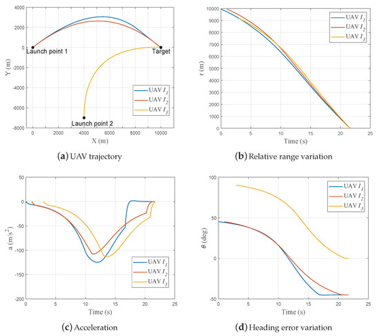
Figure 12. Simulation results of Case 3.

5. Conclusions

In this paper, a novel guidance law is proposed to control impact time and angle under variable speed based on geometric approach and inverse dynamics. Engine thrust and aerodynamic drag are involved in motion model.

Different from the time-domain-control based guidance laws with implicit flight trajectories, this paper introduces Bezier curves to design trajectories that explicitly satisfy the impact time and angle constraints. The trajectory is composed of initial and terminal phases, which correspond to a quadratic Bezier curve and a straight line, respectively. Notably, the trajectories of the two phases are tangent to each other at the phase switching point, which ensures the smooth of the entire flight trajectory. The impact angle is achieved by driving the UAV along a specified ending line in the terminal phase. This ending line formulates an impact angle which is identical to the desired one. The impact time is controlled by adjusting the trajectory length, which is further realized by tuning the position of the phase switching point. To ensure that the trajectory is flyable, an acceleration bound is considered to constrain the maximum curvature of the trajectory, which limits the phase switching point position. Thus, the impact time range is restricted. The impact time range is obtained using sequential quadratic programming method.

After obtaining the flight trajectory, inverse dynamics are used for trajectory tracking. Equations of motion are considerably interpreted during guidance law derivation. Moreover, a correction process is involved to update the trajectory according to the UAV’s current state, target position and impact constraints if the flight is affected by the presence of disturbance.

The simulation results suggest that the proposed guidance law performs well in terms of impact time and angle control in the presence of variable speed.

References

- Leondes, C.T. Guidance and Control of Aerospace Vehicles; McGraw-Hill: New York, NY, USA, 1963. [Google Scholar]
- Lawrence, A. Modern Inertial Technology: Navigation, Guidance, and Control; Springer Science & Business Media: Berlin/Heidelberg, Germany, 2012. [Google Scholar]
- Sun, W.; Liu, X.; Zheng, Z. Survey on the developments on the guidance law with impact angular constraints. Flt. Dyn. 2010, 28, 1–5. [Google Scholar]
- Chen, K.; Guo, Y.; Wang, S.C.; Xia, F. A survey on guidance law with impact time constraint. In Proceedings of the 35th Chinese Control Conference, Chengdu, China, 27–29 July 2016; IEEE: Piscataway, NJ, USA, 2016; pp. 5711–5715. [Google Scholar]
- Lee, J.I.; Jeon, I.S.; Tahk, M.J. Guidance law to control impact time and angle. IEEE Trans. Aerosp. Electron. Syst. 2007, 43, 301–310. [Google Scholar]
- Harl, N.; Balakrishnan, S. Impact time and angle guidance with sliding mode control. IEEE Trans. Control Syst. Technol. 2012, 20, 1436–1449. [Google Scholar] [CrossRef]
- Lee, C.H.; Kim, T.H.; Tahk, M.J.; Whang, I.H. Polynomial guidance laws considering terminal impact angle and acceleration constraints. IEEE Trans. Aerosp. Electron. Syst. 2013, 49, 74–92. [Google Scholar] [CrossRef]
- Kim, T.H.; Lee, C.H.; Jeon, I.S.; Tahk, M.J. Augmented polynomial guidance with impact time and angle constraints. IEEE Trans. Aerosp. Electron. Syst. 2013, 49, 2806–2817. [Google Scholar] [CrossRef]
- Zhang, Y.; Ma, G.; Liu, A. Guidance law with impact time and impact angle constraints. Chin. J. Aeronaut. 2013, 26, 960–966. [Google Scholar] [CrossRef]
- Zhao, Y.; Sheng, Y.; Liu, X. Analytical impact time and angle guidance via time-varying sliding mode technique. ISA Trans. 2016, 62, 164–176. [Google Scholar] [CrossRef]
- Livermore, R.; Shima, T. Deviated Pure-Pursuit-Based Optimal Guidance Law for Imposing Intercept Time and Angle. J. Guid. Control Dyn. 2018, 41, 1–8. [Google Scholar] [CrossRef]
- Chen, X.; Wang, J. Optimal control based guidance law to control both impact time and impact angle. Aerosp. Sci. Technol. 2019, 84, 454–463. [Google Scholar] [CrossRef]
- Chen, X.; Wang, J. Two-stage guidance law with impact time and angle constraints. Nonlinear Dyn. 2019, 95, 2575–2590. [Google Scholar] [CrossRef]
- Kang, S.; Tekin, R.; Holzapfel, F. Generalized impact time and angle control via look-angle shaping. J. Guid. Control Dyn. 2019, 42, 695–702. [Google Scholar] [CrossRef]
- Liu, X.; Li, G. Adaptive Sliding Mode Guidance With Impact Time and Angle Constraints. IEEE Access 2020, 8, 26926–26932. [Google Scholar] [CrossRef]
- Dhananjay, N.; Ghose, D. Accurate time-to-go estimation for proportional navigation guidance. J. Guid. Control Dyn. 2014, 37, 1378–1383. [Google Scholar] [CrossRef]
- Jeon, I.S.; Lee, J.I.; Tahk, M.J. Homing guidance law for cooperative attack of multiple missiles. J. Guid. Control Dyn. 2010, 33, 275–280. [Google Scholar] [CrossRef]
- Manchester, I.R.; Savkin, A.V. Circular-navigation-guidance law for precision missile/target engagements. J. Guid. Control Dyn. 2006, 29, 314–320. [Google Scholar] [CrossRef]
- Pharpatara, P.; Hérissé, B.; Pepy, R.; Bestaoui, Y. Sampling-based path planning: A new tool for missile guidance. IFAC Proc. Vol. 2013, 46, 131–136. [Google Scholar] [CrossRef]
- Fowler, L.; Rogers, J. Bezier curve path planning for parafoil terminal guidance. J. Aerosp. Inf. Syst. 2014, 11, 300–315. [Google Scholar] [CrossRef]
- Qin, Z.; Qi, X.; Fu, Y. Terminal guidance based on Bézier curve for climb-and-dive maneuvering trajectory with impact angle constraint. IEEE Access 2018, 7, 2969–2977. [Google Scholar] [CrossRef]
- Yakimenko, O.A. Direct method for rapid prototyping of near-optimal aircraft trajectories. J. Guid. Control Dyn. 2000, 23, 865–875. [Google Scholar] [CrossRef]
- Raymond, E.T.; Chenoweth, C.C. Aircraft Flight Control Actuation System Design; Society of Automotive Engineers: Warrendale, PA, USA, 1993; Volume 123. [Google Scholar]
- McLean, D. Automatic Flight Control Systems; Prentice Hall: Upper Saddle River, NJ, USA, 1990. [Google Scholar]
- Davidovitz, A.; Shinar, J. Two-target game model of an air combat with fire-and-forget all-aspect missiles. J. Optim. Theory Appl. 1989, 63, 133–165. [Google Scholar] [CrossRef]
- Alkaher, D.; Moshaiov, A. Dynamic-escape-zone to avoid energy-bleeding coasting missile. J. Guid. Control Dyn. 2015, 38, 1908–1921. [Google Scholar] [CrossRef]
- Marsh, D. Applied Geometry for Computer Graphics and CAD; Springer Science & Business Media: Berlin/Heidelberg, Germany, 2006. [Google Scholar]
- Greco, O.; Martino, I. Syzygies of the Veronese modules. Commun. Algebra 2016, 44, 3890–3906. [Google Scholar] [CrossRef][Green Version]
- Greco, O.; Martino, I. Cohen-Macaulay Property and Linearity of Pinched Veronese Rings. J. Commut. Algebra 2020, in press euclid:1552464033. [Google Scholar]
- Sapidis, N.S.; Frey, W.H. Controlling the curvature of a quadratic Bézier curve. Comput. Aided Geom. Des. 1992, 9, 85–91. [Google Scholar] [CrossRef]
© 2020 by the authors. Licensee MDPI, Basel, Switzerland. This article is an open access article distributed under the terms and conditions of the Creative Commons Attribution (CC BY) license (http://creativecommons.org/licenses/by/4.0/).