Article

Birnbaum-Saunders Quantile Regression Models with Application to Spatial Data

1
Department of Mathematics and Statistics, Universidad de La Frontera, Temuco 4780000, Chile
2
School of Industrial Engineering, Pontificia Universidad Católica de Valparaíso, Valparaíso 2362807, Chile
3
Department of Statistics, Pontificia Universidad Católica de Chile, Santiago 8320000, Chile
4
Department of Statistics, Universidade de Brasília, Brasília 70910-90, Brazil
*
Author to whom correspondence should be addressed.
Mathematics 2020, 8(6), 1000; https://doi.org/10.3390/math8061000
Submission received: 30 April 2020 / Revised: 11 June 2020 / Accepted: 12 June 2020 / Published: 18 June 2020
(This article belongs to the Special Issue Statistical Simulation and Computation)

Abstract

:
In the present paper, a novel spatial quantile regression model based on the Birnbaum–Saunders distribution is formulated. This distribution has been widely studied and applied in many fields. To formulate such a spatial model, a parameterization of the multivariate Birnbaum–Saunders distribution, where one of its parameters is associated with the quantile of the respective marginal distribution, is established. The model parameters are estimated by the maximum likelihood method. Finally, a data set is applied for illustrating the formulated model.

1. Introduction

An asymmetric distribution that has recently received considerable attention is the Birnbaum–Saunders (BS) model. It originated from material fatigue and has been applied to reliability and fatigue studies [1,2,3]. Extensive work has been done on the BS distribution with regard to its mathematical and statistical properties, inference, modeling, and diagnostics. Its natural applications have been mainly focused on engineering. However, today they range diverse fields including air pollution [4,5], business [6], earth sciences [7,8], industry [9,10], and medicine [11,12], among other areas. These applications have been performed by an international transdisciplinary group of researchers.
Standard regression models provide an estimate of the mean response given certain values of the covariates. These models cannot be applied to estimate other parameters that are different to the mean, being a limitation of such models. Nevertheless, first, in engineering, environmental, and social sciences, as well as in other areas, often the practitioners are interested in estimating quantiles for establishing warranties of products, determining the levels of nutrients in the soil or measuring economic inequality for poor (lower tail) and rich (upper tail) people by means of their household incomes [13]. Second, the other limitation of the standard regression models is that if the response variable follows a skew distribution, then the mean is not a good central tendency measure to summarize the data and, in this case, the median is a more informative and robust estimate. Additionally, third, regression models can describe parameters of the whole distribution related to variability, skewness, and other higher-order moments, which can characterize a distribution [14]. In order to solve the first two limitations mentioned above, quantile regression models were proposed by [15], extending the median regression model attributed to [16], and generalizing the ordinary sample quantiles to the regression setting. We are interested in modeling the median or other quantiles of the BS distribution by regression; see [17,18].
The accuracy of an estimator of the mean (or median) might be improved if a spatial component is added in the modeling [19]. The idea of spatial quantile regression was initially proposed by [20], and [21] discussed a general spatial quantile regression based on the conditional quantile function, while [22] showed variants of the spatial quantile regression. We provide background of quantile regression including the spatial case in the next section. Ref [23,24,25] introduced BS spatial mean regression models and their diagnostics for the conditional mean; see [26] for details on diagnostic methods. Stochastic processes are applied in the modeling of spatial data to know the corresponding finite dimensional multivariate distributions. BS multivariate distributions have been proposed and studied by [27,28,29]. BS quantile regression models were recently derived by [13] for the independent case, where household income data were considered. However, no studies on BS quantile regression for data with spatial dependence have been proposed.
The main objective of this work is to formulate a novel class of spatial quantile regression models based on the BS distribution. To accomplish this, we propose a quantile parameterization to generate a new multivariate BS model, whose parameters are estimated by the maximum likelihood method. Subsequently, a data set is applied for illustration.
The remainder paper is organized as follows. In Section 2, quantile regression models for the cases of independent and spatial data are described. Section 3 presents the univariate BS distribution in its original parameterization and a new parameterization of it, which allows us to model a quantile. In Section 4, the multivariate normal distribution and its connection to the new parametrization of the multivariate BS distribution are introduced. In Section 5, we formulate the spatial quantile regression model based on the BS distribution. Section 6 derives estimation of model parameters using the maximum likelihood method, whereas tools for model checking are discussed in Section 7. In Section 8, we carry out an empirical example with spatial data to illustrate potential applications of the novel model. Conclusions and future works are mentioned in Section 9. An Appendix A with derivatives for the score vector and Hessian matrix is provided at the end of this paper.

2. Quantile Regression

Standard regression models have been widely used in different areas and they are defined as
Y i = x i β + ε i , i = 1 , n ¯ ,
where Y is the dependent (or response) variable; x corresponds to the values of the vector of independent variables (covariates) X ; β is a vector of regression parameters; and ε is a random error with E [ ε ] = 0 , Var [ ε ] = ς 2 (constant variance), and Cov [ ε l , ε k ] = 0 , for l k (uncorrelated errors). This implies that a regression model describes the conditional mean E [ Y | X = x ] = x β , so that it can be written by the probability density function (PDF) of Y parameterized in terms of its mean. For example, if Y is normally distributed, then its linear regression model might be visualized as
Y i | X i = x i N ( μ i = x i β , ς 2 ) , i = 1 , n ¯ ,
with Y 1 | X 1 = x 1 , , Y n | X n = x n being independent random variables. Additionally, we can generalize the expression for μ i given in (1) when considering μ i = h 1 ( x i β ) , where h 1 is an invertible function, such as in generalized linear models [30]. If we now consider a k-parameter distribution, with θ = ( θ 1 = μ = h 1 ( x β ) , θ 2 , , θ k ) , that is, distributions parameterized on their mean [31,32] in addition to other parameters, one may establish a more general model of the form
Y i | X i = x i f Y ( y ; θ 1 = h 1 ( x i β ) , θ 2 , , θ k ) , i = 1 , n ¯ ,
where Y now follows some distribution.
Quantile regression models for a response Y offer a mechanism to estimate and predict the median response as well as other quantiles [15]. This class of regression models is based on the quantile function that is given by
Q Y ( τ ; θ ) = inf { y : F Y ( y ; θ ) τ } ,
where θ is a k × 1 parameter vector of the underlying distribution and 0 < τ < 1 . If one of the pararameters of the distribution of Y is its quantile function, we can represent a quantile regression model, similarly to (2), as
Y i | X i = x i f Y ( y ; Q Y ( τ ; β , x i ) = h ( x i β ) , θ 2 , , θ k ) , i = 1 , n ¯ ,
where h is an invertible function, with positive support and at least twice differentiable, τ is a fixed value and, as before, Y 1 | X 1 = x 1 , , Y n | X n = x n are independent random variables.
Let { Y ( s ) , s D } be a stochastic process that is defined over a region D R 2 . We use the notation Q Y ( s ) ( τ ; θ ) = inf { y : F Y ( s ) ( y ; θ ) τ } to represent the quantile function for Y in the location s D R 2 . If we consider spatial locations s i , the quantile function of the process can be modeled by regression as Q Y ( s i ) ( τ ; β | x ( s i ) ) = x ( s i ) β , or more generally as Q Y ( s i ) ( τ ; β | x ( s i ) ) = h 1 ( x ( s i ) β ) , for i = 1 , n ¯ . Here, Q Y i ( τ ; β | x i ) is the conditional quantile function of Y given a set of values x i for the covariates, in the location s i , where τ is a fixed value, and h is as given in (3). When τ = 0.5 , the median is modeled. Often it is assumed that the covariance function of the process only depends on the distance between spatial locations, that is, the stochastic process is stationary.

3. The Univariate Birnbaum-Saunders Distribution

If Z N ( 0 , 1 ) , then the random variable T given by
T = T ( Z ; α , ϱ ) = ϱ α Z / 2 + α Z / 2 2 + 1 2
has a BS distribution with parameters of shape α > 0 and scale ϱ > 0 , which is denoted by T BS ( α , ϱ ) . The random variable T has positive support and the transformation given in (4) is one-to-one, which allows us to establish that
Z = 1 α T / ϱ ϱ / T N ( 0 , 1 ) .
The PDF and cumulative distribution function (CDF) of T are expressed, respectively, by
f T ( t ) = ϕ ( A ( t ; α , ϱ ) ) a ( t ; α , ϱ ) , F T ( t ) = Φ ( A ( t ; α , ϱ ) ) , t > 0 ,
where ϕ , Φ are the PDF and CDF of the standard normal distribution, whereas
A ( t ; α , ϱ ) = 1 α t / ϱ ϱ / t , a ( t ; α , ϱ ) = d d t [ A ( t ; α , ϱ ) ] = 1 2 α ϱ ϱ / t + ( t / ϱ ) 3 .
Let T BS ( α , ϱ ) . Subsequently, the following properties hold:
(i)
E [ T ] = ϱ ( 1 + α 2 / 2 ) .
(ii)
Var [ T ] = ϱ 2 α 2 ( 1 + 5 α 2 / 4 ) .
(iii)
b T BS ( α , b ϱ ) , for b > 0 .
(iv)
1 / T BS ( α , 1 / ϱ ) .
(v)
W = Z 2 = ( 1 / α 2 ) ( T / ϱ + ϱ / T 2 ) χ 2 ( 1 ) , with E [ W ] = 1 and Var [ W ] = 2 .
These properties are useful for diverse statistical purposes, such as the generation of moments and of random numbers, estimation of parameters, and modeling based on regression. Another property of the BS distribution is presented next. Given q ( 0 , 1 ) , note that the qth quantile of the BS distribution is defined as
Q = t q = ϱ 4 α z q + α 2 z q 2 + 4 2 = ϱ 4 γ α 2 ,
where
γ α = α z q + α 2 z q 2 + 4 ,
with z q being the qth quantile of the standard normal distribution.

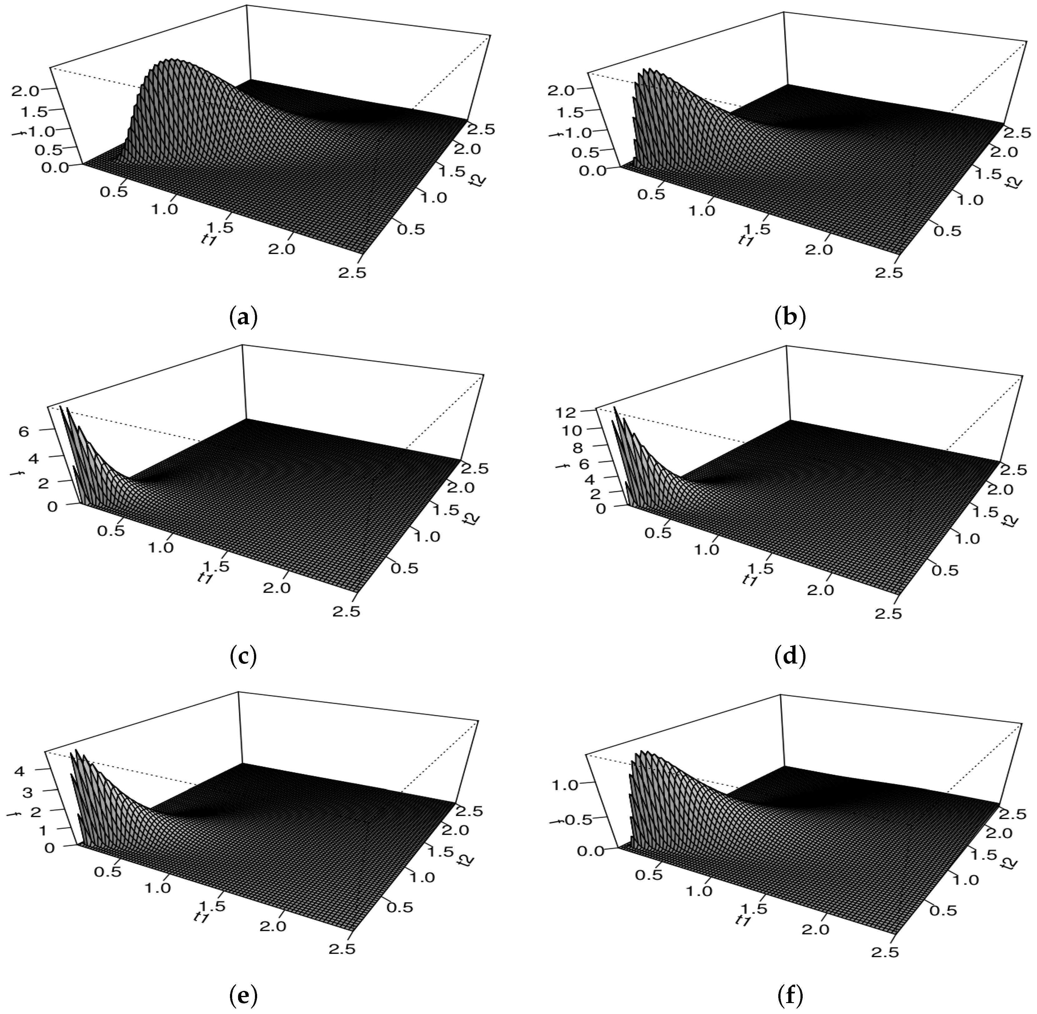
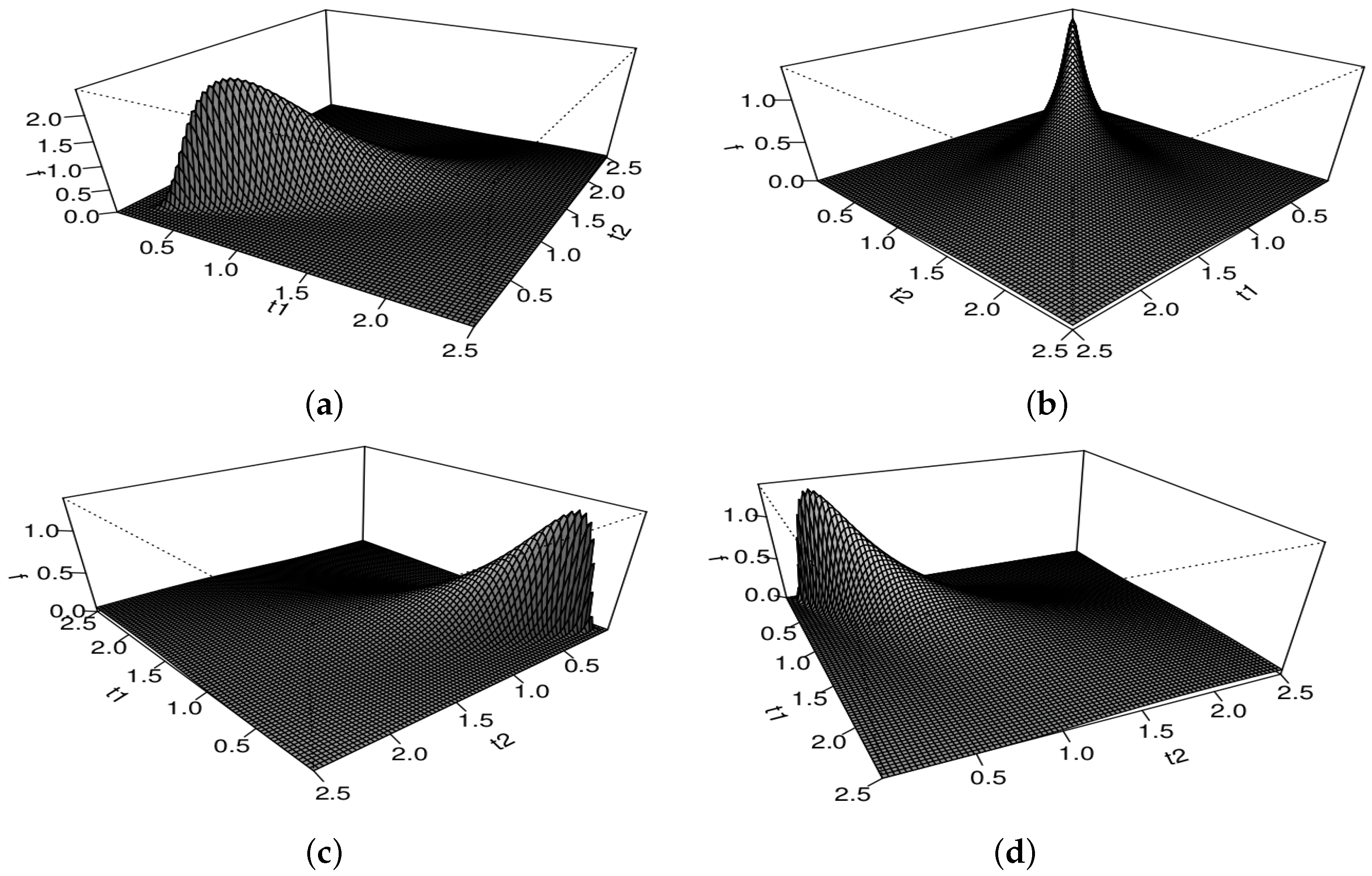
4. The Multivariate BS Distribution and a New Parametrization

Let V = ( V 1 , , V n ) R n be a random vector with n-variate normal distribution, denoted by V N n ( μ , Σ ) , with mean vector μ = ( μ i ) R n and variance-covariance matrix Σ = ( σ k l ) R n × n , with rank ( Σ ) = n . Note that Σ is symmetric, non-singular, positive definite, and then the distribution of V is non-singular [33]. When the mean vector is zero, that is, μ = 0 n × 1 , we use the notation ϕ n and Φ n for the n-variate normal PDF and CDF, respectively, where 0 n × 1 is an n × 1 vector of zeros.
The random vector T = ( T 1 , , T n ) R + n follows an n-variate BS distribution with parameters α = ( α 1 , , α n ) R + n , ϱ = ( ϱ 1 , , ϱ n ) R + n , and Σ R n × n , if T i = T ( V i ; α i , ϱ i ) , for i = 1 , n ¯ , where T is given in (4) and V = ( V 1 , , V n ) R n N n ( 0 n × 1 , Σ ) , with Σ R n × n being the variance-covariance matrix of V with diagonal elements equal to one. Therefore, Σ is also the correlation matrix of V in this case. Note that Σ is the correlation matrix of V and not of T , but we use the notation T BS n ( α , Q , Σ ) due to the relationship between the BS and normal distributions. Observe that the CDF and PDF of T BS n ( α , ϱ , Σ ) are defined, respectively, by
F T ( t ; α , ϱ , Σ ) = Φ n ( A ; Σ ) , f T ( t ; α , ϱ , Σ ) = ϕ n ( A ; Σ ) a ( t ; α , ϱ ) , t = ( t 1 , , t n ) R + n ,
where A = A ( t ; α , ϱ ) = ( A 1 , , A n ) , with A i = A ( t i ; α i , ϱ i ) , a ( t ; α , ϱ ) = i = 1 n a ( t i ; α i , ϱ i ) , and both A ( t i ; α i , ϱ i ) and a ( t i ; α i , ϱ i ) are as expressed in (5).
Let q ( 0 , 1 ) be a fixed number and T BS ( α , ϱ ) . If we apply the transformation given by
( α , ϱ ) ( α , Q )
where Q is defined in (6), then this transformation is one-to-one. Therefore, if T = ( T 1 , , T n ) BS n ( α , ϱ , Σ ) , we have a new parametrization of the multivariate BS distribution, denoted by T BS n ( α , Q , Σ ) , acting similarly as in (8) by the transformation expressed as
( α , ϱ , Σ ) ( α , Q , Σ ) ,
where the elements Q i , ϱ i of Q , ϱ are related by (6) for the marginal distribution of T i , i = 1 , n ¯ . Thus, according to (9), the CDF and PDF of T BS n ( α , Q , Σ ) are given, respectively, by
F T ( t ; α , Q , Σ ) = Φ n ( A ¯ ; Σ ) , f T ( t ; α , Q , Σ ) = ϕ n ( A ¯ ; Σ ) a ¯ ( t ; α , Q ) , t = ( t 1 , , t n ) R + n ,
where A ¯ = ( A ¯ 1 , , A ¯ n ) , with A ¯ i = A ( t i ; α i , 4 Q i / γ α i 2 ) = [ 1 / ( α i γ α i 4 Q i t i ) ] ( t i γ α i 2 / 4 Q i 1 ) , a ¯ ( t ; α , Q ) = j = 1 n a ( t i ; α i , 4 Q i / γ α i 2 ) = j = 1 n [ 1 / ( α i γ α i 4 Q i t i ) ] ( γ α i 2 / 2 + 2 Q i / t i ) , and γ α i being defined in (7). Figure 1 and Figure 2 present different graphical plots for the PDF defined in (10) with n = 2 , when the parameters α and Q vary, for different rotations of these PDFs.
Theorem 1.
Let T = ( T 1 , , T n ) BS n ( α , Q , Σ ) , with α = ( α 1 , , α n ) , Q = Q 1 , , Q n , and Σ = ( σ k l ) being an n × n correlation matrix. Afterwards,
(i) 
T i BS ( α i , Q i ) , for i = 1 , n ¯ .
(ii) 
( T i , T j ) BS 2 ( α ( i , j ) , Q ( i , j ) , Σ ( i , j ) ) , where α ( i , j ) = ( α i , α j ) , Q ( i , j ) = ( Q i , Q j ) and Σ ( i , j ) is a 2 × 2 matrix with ones in its diagonal and its other elements equal to element ( i , j ) of the matrix Σ.
(iii) 
Cov [ T i , T j ] = 4 α i α j Q i Q j γ α i 2 γ α j 2 α i α j σ i j 2 + 4 I ( α i , α j , σ i j ) , i , j = 1 , n ¯ ,
where I ( α i , α j , σ i j ) = E { Z i Z j [ ( α i Z i / 2 ) 2 + 1 ] 1 / 2 [ ( α j Z j / 2 ) 2 + 1 ] 1 / 2 } , with ( Z i , Z j ) following a bivariate normal distribution and correlation matrix Σ ( i , j ) ; see [34].
(iv) 
The variance-covariance matrix of T is Var [ T ] = 4 Ω Σ Σ Ξ + 4 U , where Ω = ( ω i j ) , Ξ = ( ξ i j ) and U = ( u i j ) have elements ω i j = α i 2 α j 2 Q i Q j / ( γ α i 2 γ α j 2 ) , ξ i j = α i α j and u i j = I ( α i , α j , σ i j ) , respectively, for i , j = 1 , n ¯ , and is the Hadamard product. If T 1 , , T n are independent random variables, then Var [ T ] = 4 D ( ϵ i i ) , where D ( ϵ i i ) = diag ( ϵ 11 , , ϵ n n ) , that is, D is a diagonal matrix with elements ϵ i i = α i 2 Q i 2 ( α i 2 + 4 I ( α i , α i , 1 ) ) / γ α i 4 .
Proof. 
The results are deduced using Theorem 3.1 and p. 117 of [34], with our parametrization. ☐
Corollary 1.
Let T = ( T 1 , T 2 ) BS 2 ( α , Q , Σ ) , with α = ( α 1 , α 2 ) , Q = ( Q 1 , Q 2 ) and Σ = 1 σ σ 1 . Then,
(i) 
E [ T 1 T 2 ] = 4 Q 1 Q 2 γ α 1 2 γ α 2 2 4 + 2 ( α 1 2 + α 2 2 ) + α 1 2 α 2 2 ( 1 + σ 2 ) + 4 α 1 α 2 I ( α 1 , α 2 , σ ) ,
with I ( α 1 , α 2 , σ ) being defined in Theorem 1(iii).
(ii) 
Cov [ T 1 , T 2 ] = 4 σ 2 α 1 α 2 Q 1 Q 2 γ α 1 2 γ α 2 2 α 1 α 2 σ 2 + 4 I ( α 1 , α 2 , σ ) .
(iii) 
Corr ( T 1 , T 2 ) = α 1 α 2 σ 2 + 4 I ( α 1 , α 2 , σ ) 4 + 5 α 1 2 4 + 5 α 2 2 .
Proof. 
The results are obtained using ([34] p.117), with our parametrization; see also [35]. ☐

5. Formulation of the Spatial Model

Let T = { T ( s ) , s D } be a stochastic process that is defined over a region D R 2 . We assume that the stochastic process T is stationary and isotropic, and that, for given spatial locations s i , with i = 1 , n ¯ , the quantile function of the process can be modeled by
Q ( T ( s i ) ; β | x i ) = Q i = h 1 ( x i β ) , i = 1 , n ¯ ,
where h is an invertible function, with positive support, at least twice differentiable, and x i = ( 1 , x i 1 , , x i ( p 1 ) ) represents the values of p 1 covariates, with x i j = x j ( s i ) , for j = 1 , p 1 ¯ , that is, x i j is the value of the covariate X j at the location s i . Note that p < n must be satisfied. In addition, β = ( β 0 , β 1 , , β p 1 ) is a vector of unknown parameters to be estimated and ( T ( s 1 ) , , T ( s n ) ) = ( T 1 , , T n ) BS n ( α 1 n × 1 , Q ( β ) , Σ ) , with α > 0 and 1 n × 1 being an n × 1 vector of ones. Observe that Q ( β ) is related to Q defined in (9), but now depending on β . Here, Σ = ( σ i j ) is the n × n (non-singular) correlation matrix earlier defined. Thus, based on Theorem 1(iv), the variance-covariance matrix of the BS spatial quantile regression model can be written as
Var [ T ] = 4 α 2 γ α 4 [ Q ( β ) Q ( β ) ] ( α 2 Σ Σ + 4 U ) ,
where Q ( β ) = ( Q 1 ( β ) , , Q n ( β ) ) , with Q i ( β ) = h 1 ( x i β ) , for i = 1 , n ¯ . Notice that the variance-covariance matrix of the BS spatial process that is stated in (12) depends on its quantile function.
Note that the spatial correlation is often modeled by a function of the Matérn family [19]. Subsequently, by using this family and an alternative parameterization suggested by [36], the elements of the matrix Σ involved in (12) are given by
σ i j = 1 , i = j ; 1 2 δ 1 Γ ( δ ) ( φ h i j ) δ K δ ( φ h i j ) , i j ;
where δ > 0 is a shape parameter; Γ is the usual gamma function; h i j is the Euclidean distance between the locations s i and s j , that is, h i j = | | s i s j | | ; φ > 0 is a parameter known as the spatial dependence inverse radius [37] and also related to a parameter named microergodic by [36]; and, K δ is the modified Bessel function of the third kind of order δ [38]. Some particular cases of the Matérn family are presented in Table 1.

6. Estimation of Model Parameters
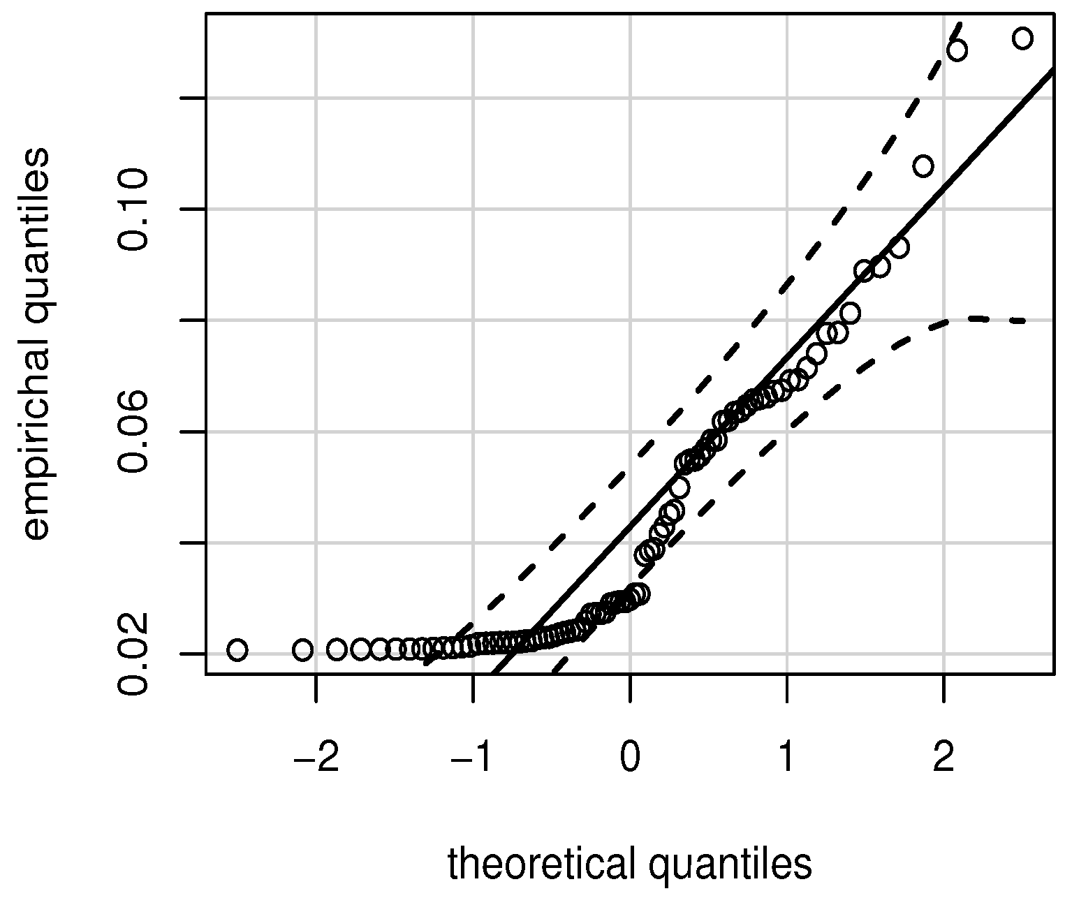
Let θ = ( α , β , φ ) be a vector of unknown parameters of the spatial quantile regression model formulated in (11), which can be estimated by the maximum likelihood method, as follows. Note that φ > 0 is the spatial dependence inverse radius [39] of the Matérn spatial correlation function defined in (13). Therefore, the corresponding log-likelihood function for θ based on the vector of observations t = ( t 1 , , t n ) can be written as
( θ ) = n 2 log ( 2 π ) 1 2 log ( | Σ | ) 1 2 A ¯ Σ 1 A ¯ + log ( a ¯ ) ,
where A ¯ = A ¯ ( t ; α 1 n × 1 , Q ) , with Q = Q ( β ) , a ¯ = a ¯ ( t ; α 1 n × 1 , Q ) , and Σ involved in (12). Taking the derivative of (14), with respect to the corresponding parameters, leads to the ( p + 2 ) × 1 score vector that is defined as
˙ ( θ ) = ( θ ) α , ( θ ) β , ( θ ) φ = ˙ α , ˙ β 0 , ˙ β 1 , , ˙ β p 1 , ˙ φ .
For details of the score vector given in (15), see the Appendix A. In order to find the maximum likelihood estimate θ ^ of θ , the non-linear system ˙ ( θ ) = 0 ( p + 2 ) × 1 must be solved. Because this system does not provide a closed analytical solution, θ ^ must be computed using an iterative procedure for non-linear systems. Here, a quasi-Newton procedure, named Broyden-Fletcher-Goldfarb-Shanno [40,41], may be used through the functions optim and optimx implemented in the R software; see www.R-project.org and [42]. The signs of the determinants of the corresponding Hessian matrix and of its minors were also checked to ensure that a valid maximum has been attained.
Note that the Hessian matrix ¨ ( θ ) for the BS spatial quantile regression model is a ( p + 2 ) × ( p + 2 ) diagonal block matrix. This Hessian matrix is obtained by taking the second derivative of (14), with respect to the corresponding parameters, and it is given by
¨ ( θ ) = 2 ( θ ) α 2 2 ( θ ) α β 2 ( θ ) α φ 2 ( θ ) β α 2 ( θ ) β β 2 ( θ ) β φ 2 ( θ ) φ α 2 ( θ ) φ β 2 ( θ ) φ 2 = ¨ α α ¨ α β ¨ α φ ¨ β α ¨ β β ¨ β φ ¨ φ α ¨ φ β ¨ φ φ ,
where the elements of the matrix ¨ ( θ ) are detailed in the Appendix A. Therefore, for the BS spatial quantile regression model, the ( p + 2 ) × ( p + 2 ) expected Fisher information matrix, as obtained from (16), is expressed as
K ( θ ) = E [ ¨ ( θ ) ] = K α α K α β K α φ K β α K β β K β φ K φ α K φ β K φ φ ,
where the elements of the matrix K ( θ ) are detailed in the Appendix A as well.

7. Model Checking

We consider a property of the multivariate BS distribution related to the Mahalanobis distance in order to evaluate the fit of the spatial model, which might be used to validate the model in practice. Let
u i = A ¯ ( i ) Σ 1 A ¯ ( i ) , i = 1 , n ¯ ,
where A ¯ ( i ) = ( A ¯ 1 ( i ) , , A ¯ n ( i ) ) , with
A ¯ j ( i ) = 1 α i γ α i 4 h 1 ( x i β ^ ( i ) ) t i t i γ α i 2 4 h 1 ( x i β ^ ( i ) ) 1 , j = 1 , n ¯ ,
and β ^ ( i ) being the maximum likelihood estimate of β obtained using the data set without the case i. A Newton–Raphson one-step approximation to θ ^ ( i ) can be obtained by
θ ^ ( i ) = θ ^ [ ¨ ( i ) ( θ ^ ) ] 1 ˙ ( i ) ( θ ^ ) , i = 1 , n ¯ ,
where ¨ ( i ) ( θ ) and ˙ ( i ) ( θ ) are the Hessian matrix and score vector of the BS spatial quantile regression model with its parameters estimated by the maximum likelihood method without the case i. Subsequently, under the assumption T BS n ( α 1 n × 1 , Q ( β ) , Σ ) , u i defined in (17) is an observation of a random variable that follows approximately a χ 2 distribution with n 1 degrees of freedom, for i = 1 , n ¯ . Thus, by using the Wilson–Hilferty approximation [43], we have that
z i = u i n 1 1 / 3 1 2 9 ( n 1 ) 2 9 ( n 1 ) 1 / 2 , i = 1 , n ¯ ,
is an observation of a random variable which follows approximately a standard normal distribution. Hence, a plot of theoretical versus empirical quantiles (QQ) for z i given in (18) can be used to evaluate the model fit. In addition to the approximation of Wilson–Hilferty, the randomized quantile residual defined by [44] may be employed to evaluate the fit of the BS spatial quantile regression model. In the case of this model, such a residual is given by
r i = Φ 1 [ F ( u i ) ] , i = 1 , n ¯ ,
where Φ 1 is the inverse N(0, 1) CDF and F is the χ 2 ( n 1 ) CDF. Because the randomized quantile residual has approximately a N(0, 1) distribution, a QQ plot of r i defined in (19) might also be employed for evaluating the model fit.

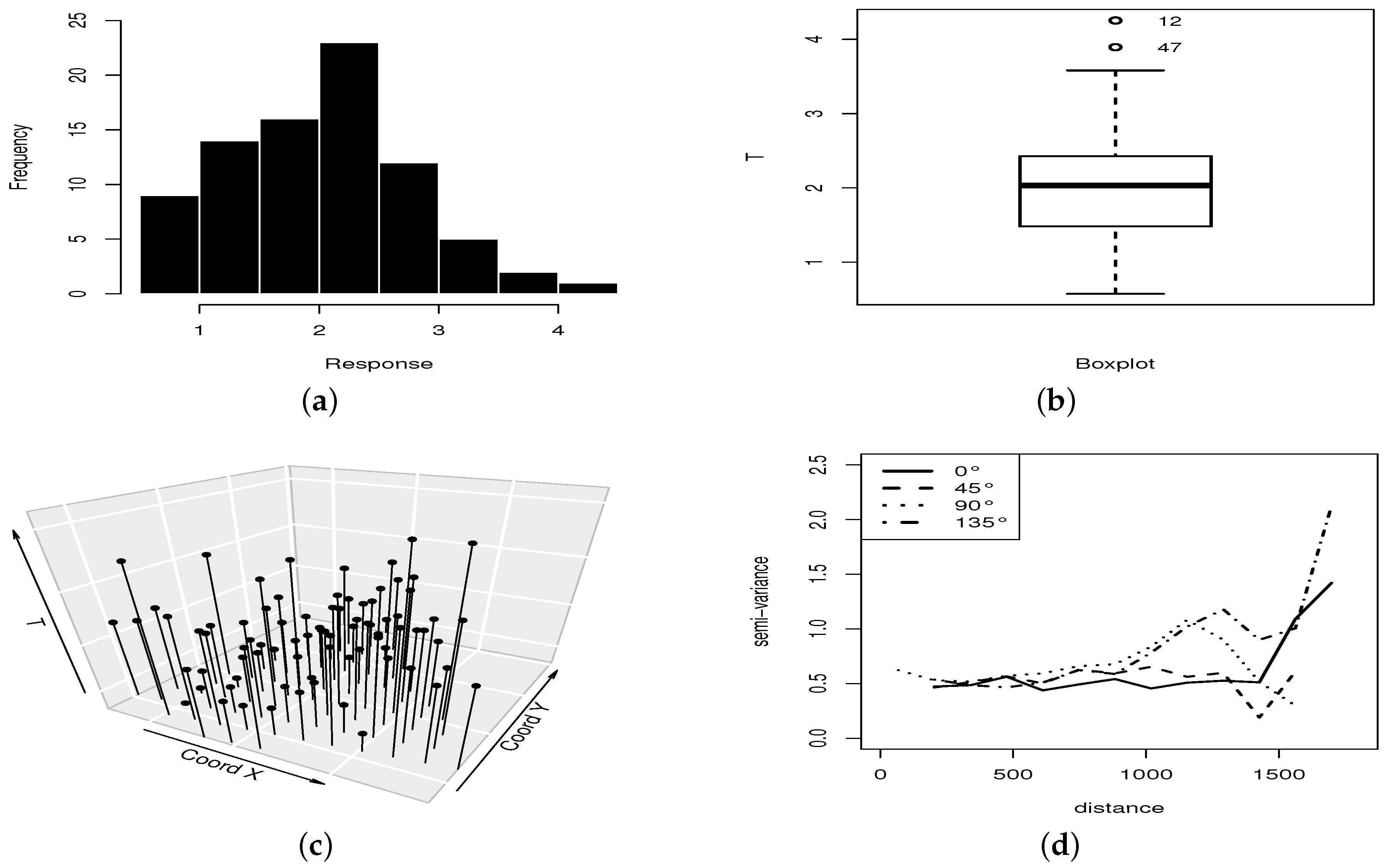
8. Empirical Illustrative Example

We analyze a chemical data set associated with imbalances and deficiencies of key nutrients in the soil in order to illustrate the results obtained in this paper. This data set corresponds to levels of magnesium (Mg), which affects the development of the root system, and calcium (Ca) that competes with Mg for absorption of nutrients, for n = 82 locations of an area in Brazil. The response variable (T) is the content of Mg in the soil (in cmolc/dm3) and the covariate (X) is the content of Ca in the soil (in cmolc/dm3).
A descriptive summary of the response variable includes the sample values (in cmolc/dm3) of the median = 2.0306; mean = 2.008; standard deviation = 0.7713; coefficient of variation = 0.3841; coefficient of skewness = 0.3394; coefficient of kurtosis = 2.9717; minimum = 0.5734; and, maximum = 4.2538. Figure 3 shows the histogram (a), boxplot (b), and scatterplot (c) of the values of the response T. In the boxplot, we detect two outliers that correspond to locations #12 and #47. The directional variogram in Figure 3d shows that there is no preferred direction, that is, an omni-directional semi-variogram is appropriate. Thus, the associated stochastic process can be considered as isotropic.
In order to estimate the parameters of BS spatial quantile regression model, we consider the following: (i) the spatial correlation is obtained according to the Matérn function (with δ = 0.5 ; see Table 1); (ii) the random vector ( T ( s 1 ) , , T ( s 82 ) ) = ( T 1 , , T 82 ) BS 82 ( α 1 82 × 1 , Q ( β ) , Σ ) is assumed; (iii) q = 0.5 (the quantile to model the median); and, (iii) the identity, logarithm, and square root functions for the link h of the spatial quantile regression defined in (11) are used and expressed as
Q i = x i β , log ( Q i ) = x i β , Q i = x i β , i = 1 , 82 ¯ ,
where β = ( β 0 , β 1 ) is the regression coefficient vector and x i = ( 1 , x i ) , with x i being the value of X for the location i.
We can compare spatial regression models while using the corrected Akaike information criterion (CAIC) and the Schwarz Bayesian information criterion (BIC). The CAIC and BIC are given, respectively, by
CAIC = 2 d 2 ( θ ^ ) + ( 2 d 2 + 2 d ) / ( n d 1 ) , BIC = d log ( n ) 2 ( θ ^ ) ,
where ( θ ^ ) is the log-likelihood function for the parameter θ associated with the model evaluated at θ = θ ^ , d is the dimension of the parameter space, and n is the size of the data set. Both criteria are based on the log-likelihood function and penalize the model with more parameters. A model whose information criterion has a smaller value is better [45]. The log-likelihood, CAIC, and BIC values for the model with links defined in (20) are presented in Table 2. Additionally, we fit a Gaussian spatial regression to the data set, which considers the modeling of the mean = median (symmetric case), allowing us to compare the models that are given in (20). Note that the BS model with square root link is better than the Gaussian model. From this table, we conclude that the BS spatial quantile regression with square root link function should be selected.
The maximum likelihood estimates of the selected model parameters and the corresponding asymptotic standard errors, estimated by using the robust covariance matrix method [46] and reported in parentheses, are:
α ^ = 0.2323 ( 0.0460 ) , β ^ 0 = 0.3821 ( 0.0030 ) , β ^ 1 = 0.1884 ( 0.0093 ) , φ ^ = 0.0045 ( 0.0021 ) .
These standard errors are low, indicating that all of the parameters are estimated with good statistical precision and allow us to infer they must be part of the model. Based on (13), note that the parameter φ is significant at 5% using the confidence interval-method, which means that exists spatial dependence. Therefore, the estimated BS spatial quantile regression model is given by
Q ^ i = ( 0.3821 + 0.1884 x i ) 2 , i = 1 , 82 ¯ ,
where the correlation matrix is determined as Σ ^ = Σ ( δ , φ ^ ) , for δ = 0.5 and evaluated at φ ^ = 0.0045 , whereas the variance-covariance matrix of the BS spatial quantile regression model defined in (12) is estimated as
Var [ T ] ^ = 4 α ^ 2 γ α ^ 4 ( Q ( β ) ^ Q ( β ) ^ ) α ^ 2 Σ ^ Σ ^ + 4 U ^ ,
where γ α ^ corresponds to γ α evaluated at α ^ = 0.2323 , Q ( β ) ^ = ( Q ^ 1 , , Q ^ 82 ) and U ^ is obtained evaluating U at α ^ and φ ^ .
Figure 4 provides the QQ plot of the residuals, transformed by the Wilson–Hilferty approximation, after removing a location that was outside the bands. Note that most of the residuals are inside of the bands. Additionally, Figure 5a displays a three-dimensional scatterplot that shows the estimated and observed values of T. These same values are presented in a two-dimensional scatterplot in Figure 5b. These plots allow us to observe a good fit of our model to the data. Therefore, we conclude that the BS spatial quantile regression model is adequate to describe these spatial data, but a better fitting could be obtained if a heavy-tailed asymmetric distribution is considered, such as the BS-Student-t distribution. However, this is beyond of the objective of the present study and it provides a challenge for further research.

9. Conclusions and Future Works

In this paper, we have obtained the following findings:
(i)
A new parameterization of the multivariate Birnbaum-Saunders distribution has been established.
(ii)
A novel Birnbaum–Saunders spatial quantile regression model has been proposed and derived.
(iii)
We have developed maximum likelihood estimation for the parameters of the proposed model.
(iv)
A randomized quantile residual has been used for model checking. We have utilized the Wilson–Hilferty approximation for our spatial model residuals to evaluate adequacy model.
(v)
The obtained results have been applied to a real data set illustrating its potential usages.
Therefore, we have derived a novel class of spatial quantile regression, which is useful for modeling data generated from a positive skew distribution. The main feature of this spatial regression is the modeling of a quantile for a response variable that follows the Birnbaum–Saunders distribution. The numerical results have reported the good performance of the spatial quantile regression model, indicating that the Birnbaum–Saunders distribution is a good modeling choice when dealing with data that have spatial dependence, positive support and follow a distribution skewed to the right. Hence, it can be a valuable addition to the tool-kit of applied statisticians and data scientists.
The following aspects are open problems for the Birnbaum–Saunders spatial quantile regression models and they can be considered for future work:
(i)
A global test for independence might be stated based on H 0 : σ i j = 0 (or Σ = I n , the n × n identity matrix). Specifically, let L full be the likelihood function for the full model and L reduced be the likelihood function for the reduced model (under H 0 indicating independence). Subsequently, we can use the likelihood ratio statistic Λ = L reduced / L full to test H 0 . Thus, instead of using the asymptotic distribution of 2 log ( Λ ) , which is unknown, a bootstrap test can be employed.
(ii)
In addition, we can consider H 0 : φ = 0 versus H 1 : φ > 0 . In this case, the asymptotic distribution of 2 log ( Λ ) under H 0 is an equally weighted mixture of chi-square distributions with zero and one degree of freedom, whose critical value is 2.7055 at a significance level of 5% [47]. In the spatial case, such a distribution might also be unknown, so that the bootstrap technique can be employed.
(iii)
it is of interest to study details of the asymptotic behavior and performance of maximum likelihood estimators [48]. However, applicability of asymptotic frameworks to spatial data is not an easy aspect. This is due to there being at least two relevant frameworks, which can behave quite differently when estimating the spatial dependence parameters; see details about these asymptotic frameworks and their implications in [49].
(iv)
The Birnbaum–Saunders distribution is based on the normal distribution and then parameter estimation in spatial quantile regression models can be affected by atypical cases. Thus, robust estimation to these cases, for example based on the Birnbaum–Saunders-t distribution, can be considered to decrease their effects; see [50].
(v)
Besides fixed effects that are added to the modeling by regression, random effects can also be added by mixed models, which may produce a more sophisticated Birnbaum-Saunders spatial quantile regression model and closer to reality [51].
(vi)
Local influence diagnostics can be conducted for Birnbaum–Saunders spatial quantile regression, which permits the detection of individual or combined influence of cases. Works on local influence in Birnbaum–Saunders models were conducted by a number of authors; see, for example, [18,23,25,52].
Research on these issues is in progress and their findings will be reported in future articles.

Author Contributions

All authors contributed with results and ideas when writing this paper. All authors have read and agreed to the published version of the manuscript.

Funding

The research was partially supported by the project grants “FONDECYT 1200525” from the National Commission for Scientific and Technological Research of the Chilean government (V. Leiva) and “Puente 001/2019” from the Research Directorate of the Vice President for Research of the Pontificia Universidad Católica de Chile, Chile (M. Galea).

Acknowledgments

The authors would also like to thank the Editor and Reviewers for their constructive comments which led to improve the presentation of the manuscript.

Conflicts of Interest

The authors declare no conflict of interest.

Appendix A. Score Vector and Fisher Information Matrix

Appendix A.1. Score Vector

The elements of the ( p + 2 ) × 1 score vector given in (15) are detailed as
˙ α = A ¯ Σ 1 A ¯ α + α [ log ( a ¯ ) ] , ˙ β j = A ¯ Σ 1 A ¯ β j + β j [ log ( a ¯ ) ] , ˙ φ = 1 2 tr Σ 1 Σ φ + 1 2 A ¯ Σ 1 Σ φ Σ 1 A ¯ ,
where A ¯ / α = ( A ¯ k / α ) and A ¯ / β k = ( A ¯ k / β j ) , with
A ¯ k α = 4 Q k t k γ α t k 2 α Q k 1 ( α γ α ) 2 ( γ α + α γ α ) t k γ α 2 4 Q k 1 , A ¯ k β j = 1 α γ α t k Q k t k γ α 2 4 Q k + 1 1 h ( Q k ) x k j , α [ log ( a ¯ ) ] = n α γ α ( γ α + α γ α ) + k = 1 n 2 t k γ α γ α t k γ α 2 + 4 Q k , β j [ log ( a ¯ ) ] = k = 1 n 1 2 Q k + 4 t k γ α 2 + 4 Q k 1 h ( Q k ) x k j .
In addition, Σ / φ = ( σ i j / φ ) , with elements defined as
σ i j φ = h i j δ 2 δ 1 Γ ( δ ) δ φ δ 1 K δ ( φ h i j ) + φ δ K δ ( φ h i j ) h i j , i j ; 0 , i = j ;
where K δ ( u ) = d K δ ( u ) / d u .

Appendix A.2. Information Matrix

To obtain the Fisher information matrix, ¨ ( θ ) must be evaluated at θ = θ ^ . For the BS spatial quantile regression model presented in (11), the elements of the Hessian matrix can be expressed as
¨ β j β l = A ¯ β l Σ 1 A ¯ β j + A ¯ Σ 1 2 A ¯ β j β l + β l log ( a ˜ ) β j , ¨ β j φ = A ¯ Σ 1 Σ φ Σ 1 A ¯ β j , ¨ φ φ = 1 2 φ tr Σ 1 Σ φ + 1 2 A ¯ Σ 1 Σ φ Σ 1 Σ φ + Σ 1 2 Σ φ 2 Σ 1 Σ 1 Σ φ Σ 1 Σ φ Σ 1 A ¯ ,
where
2 A ˜ k β j β l = 1 α γ α t k Q k 3 t k γ α 2 8 Q k 2 + 1 2 Q k 1 h ( Q k ) + t k γ α 2 4 Q k + 1 h ( Q k ) [ h ( Q k ) ] 2 1 h ( Q k ) x k j x k l , β l log ( a ˜ ) β j = k = 1 n 1 2 Q k 2 16 ( t k γ α 2 + 4 Q k ) 2 1 [ h ( Q k ) ] + 1 2 Q k 4 t k γ α 2 + 4 Q k h ( Q k ) [ h ( Q k ) ] 2 1 h ( Q k ) x k j x k l ,
and 2 Σ / φ 2 = ( 2 σ i j / φ 2 ) , whose elements are given by
2 σ i j φ 2 = h i j δ φ δ 2 2 δ 1 Γ ( δ ) δ ( δ 1 ) K δ ( φ h i j ) + δ φ K δ ( φ h i j ) i j ; + δ φ K δ ( φ h i j ) + φ 2 K δ ( φ h i j ) h i j , 0 , i = j ;
with K δ ( u ) = d 2 K δ ( u ) / d u 2 . In addition, the p × 1 and 3 × 1 vectors ¨ β α = [ ¨ α β ] and ¨ φ α = [ ¨ α φ ] , respectively, have elements given by
¨ α β j = A ¯ β j Σ 1 A ¯ α + A ¯ Σ 1 2 A ¯ α β j + α log ( a ˜ ) β j , ¨ α φ = A ¯ Σ 1 Σ φ Σ 1 A ¯ α ,
where 2 A ¯ / α β j = ( 2 A ˜ k / α β j ) , with
2 A ˜ k α β j = 1 ( α γ α ) 2 ( γ α + α γ α ) t k γ α 2 4 Q k + 1 1 α γ α t k γ α γ α 2 Q k × 1 t k Q k 1 h ( Q k ) x k j , α log ( a ˜ ) β j = k = 1 n 8 t k γ α γ α ( t k γ α 2 + 4 Q k ) 2 1 h ( Q k ) x k j .
Furthermore, we have
¨ α α = A ¯ α Σ 1 A ¯ α + A ¯ Σ 1 2 A ¯ α 2 + 2 log ( a ˜ ) α 2 ,
where 2 A ¯ / α 2 = ( 2 A ˜ k / α 2 ) , with
2 A ˜ k α 2 = 4 Q k t k t k γ α 2 4 Q k 1 2 ( α γ α ) 3 ( γ α + α γ α ) 2 2 γ α + α γ α ( α γ α ) 2 ( γ α + α γ α ) t k γ α γ α 2 Q k ( α γ α ) 2 + t k 2 Q k γ α α γ α α 2
and
2 log ( a ˜ ) α 2 = n ( 2 γ α + α γ α ) ( α γ α ) ( γ α + α γ α ) 2 ( α γ α ) 2 + k = 1 n 2 t k ( [ γ α ] 2 + γ α γ α ) ( t k γ α 2 + 4 Q k ) 2 t k γ α 2 ( γ α ) 2 ( t k γ α 2 + 4 Q k ) 2 .

References

  1. Arrue, J.; Arellano-Valle, R.B.; Gomez, H.W.; Leiva, V. On a new type of Birnbaum-Saunders models and its inference and application to fatigue data. J. Appl. Stat. 2020. [Google Scholar] [CrossRef]
  2. Khan, M.Z.; Khan, M.F.; Aslam, M.; Mughal, A.R. Design of fuzzy sampling plan using the Birnbaum-Saunders distribution. Mathematics 2019, 7, 9. [Google Scholar] [CrossRef] [Green Version]
  3. Leiva, V.; Saunders, S.C. Cumulative damage models. In Wiley StatsRef: Statistics Reference Online; Wiley: Hoboken, NJ, USA, 2015; pp. 1–10. [Google Scholar]
  4. Marchant, C.; Leiva, V.; Cysneiros, F.J.A.; Liu, S. Robust multivariate control charts based on Birnbaum-Saunders distributions. J. Stat. Comput. Simul. 2018, 88, 182–202. [Google Scholar] [CrossRef]
  5. Cavieres, M.F.; Leiva, V.; Marchant, C.; Rojas, F. A methodology for data-driven decision making in the monitoring of particulate matter environmental contamination in Santiago of Chile. Rev. Environ. Contam. Toxicol. 2020. [Google Scholar] [CrossRef]
  6. Leiva, V.; Santos-Neto, M.; Cysneiros, F.J.A.; Barros, M. A methodology for stochastic inventory models based on a zero-adjusted Birnbaum-Saunders distribution. Appl. Stoch. Model. Bus. Ind. 2016, 32, 74–89. [Google Scholar] [CrossRef]
  7. Carrasco, J.M.F.; Figueroa-Zuniga, J.I.; Leiva, V.; Riquelme, M.; Aykroyd, R.G. An errors-in-variables model based on the Birnbaum-Saunders and its diagnostics with an application to earthquake data. Stoch. Environ. Res. Risk Assess. 2020, 34, 1–12. [Google Scholar] [CrossRef]
  8. Martinez, S.; Giraldo, R.; Leiva, V. Birnbaum-Saunders functional regression models for spatial data. Stoch. Environ. Res. Risk Assess. 2019, 33, 1765–1780. [Google Scholar] [CrossRef]
  9. Huerta, M.; Leiva, V.; Liu, S.; Rodriguez, M.; Villegas, D. On a partial least squares regression model for asymmetric data with a chemical application in mining. Chemom. Intell. Lab. Syst. 2019, 190, 55–68. [Google Scholar] [CrossRef]
  10. Leiva, V.; Aykroyd, R.G.; Marchant, C. Discussion of “Birnbaum-Saunders distribution: A review of models, analysis, and applications” and a novel multivariate data analytics for an economics example in the textile industry. Appl. Stoch. Model. Bus. Ind. 2019, 35, 112–117. [Google Scholar] [CrossRef]
  11. Leao, J.; Leiva, V.; Saulo, H.; Tomazella, V. Incorporation of frailties into a cure rate regression model and its diagnostics and application to melanoma data. Stat. Med. 2018, 37, 4421–4440. [Google Scholar] [CrossRef]
  12. Leao, J.; Leiva, V.; Saulo, H.; Tomazella, V. A survival model with Birnbaum-Saunders frailty for uncensored and censored cancer data. Braz. J. Probab. Stat. 2018, 32, 707–729. [Google Scholar] [CrossRef] [Green Version]
  13. Sánchez, L.; Leiva, V.; Galea, M.; Saulo, H. Birnbaum-Saunders quantile regression and its diagnostics with application to economic data. Appl. Stoch. Models Bus. Ind. 2020. [Google Scholar] [CrossRef]
  14. Ventura, M.; Saulo, H.; Leiva, V.; Monsueto, S. Log-symmetric regression models: Information criteria, application to movie business and industry data with economic implications. Appl. Stoch. Model. Bus. Ind. 2019, 34, 963–977. [Google Scholar] [CrossRef]
  15. Koenker, R.; Bassett, G. Regression quantiles. Econometrica 1978, 46, 33–50. [Google Scholar] [CrossRef]
  16. Laplace, P. Th’eorie Analytique des Probabilit’es; Editions Jacques Gabayr: Paris, France, 1818. [Google Scholar]
  17. Dasilva, A.; Dias, R.; Leiva, V.; Marchant, C.; Saulo, H. Birnbaum-Saunders regression models: A comparative evaluation of three approaches. J. Stat. Comput. Simul. 2020, in press. [Google Scholar]
  18. Saulo, H.; Leao, J.; Leiva, V.; Aykroyd, R.G. Birnbaum-Saunders autoregressive conditional duration models applied to high-frequency financial data. Stat. Pap. 2019, 60, 1605–1629. [Google Scholar] [CrossRef] [Green Version]
  19. Diggle, P.; Ribeiro, P. Model-Based Geoestatistics; Springer: New York, NY, USA, 2007. [Google Scholar]
  20. Kostov, P. A spatial quantile regression hedonic model of agricultural land prices. Spat. Econ. Anal. 2009, 4, 53–72. [Google Scholar] [CrossRef]
  21. Trzpiot, G. Spatial quantile regression. Comp. Econ. Res. 2013, 15, 265–279. [Google Scholar] [CrossRef]
  22. McMillen, D. Quantile Regression for Spatial Data; Springer: New York, NY, USA, 2013. [Google Scholar]
  23. Garcia-Papani, F.; Uribe-Opazo, M.A.; Leiva, V.; Aykroyd, R.G. Birnbaum-Saunders spatial modelling and diagnostics applied to agricultural engineering data. Stoch. Environ. Res. Risk Assess. 2017, 31, 105–124. [Google Scholar] [CrossRef] [Green Version]
  24. Garcia-Papani, F.; Leiva, V.; Ruggeri, F.; Uribe-Opazo, M.A. Kriging with external drift in a Birnbaum-Saunders geostatistical model. Stoch. Environ. Res. Risk Assess. 2018, 32, 1517–1530. [Google Scholar] [CrossRef]
  25. Garcia-Papani, F.; Leiva, V.; Uribe-Opazo, M.A.; Aykroyd, R.G. Birnbaum-Saunders spatial regression models: Diagnostics and application to chemical data. Chemom. Intell. Lab. Syst. 2018, 177, 114–128. [Google Scholar] [CrossRef] [Green Version]
  26. Liu, Y.; Mao, G.; Leiva, V.; Liu, S.; Tapia, A. Diagnostic analytics for an autoregressive model under the skew-normal distribution. Mathematics 2020, 8, 693. [Google Scholar] [CrossRef]
  27. Sánchez, L.; Leiva, V.; Caro-Lopera, F.J.; Cysneiros, F.J.A. On matrix-variate Birnbaum-Saunders distributions and their estimation and application. Braz. J. Probab. Stat. 2015, 29, 790–812. [Google Scholar] [CrossRef]
  28. Kundu, D. Bivariate sinh-normal distribution and a related model. Braz. J. Probab. Stat. 2015, 20, 590–607. [Google Scholar] [CrossRef]
  29. Kundu, D.; Balakrishnan, N.; Jamalizadeh, A. Generalized multivariate Birnbaum-Saunders distributions and related inferential issues. J. Multivar. Anal. 2013, 116, 230–244. [Google Scholar] [CrossRef]
  30. Dobson, A. An Introduction to Statistical Modelling; Chapman and Hall: New York, NY, USA, 2002. [Google Scholar]
  31. Leiva, V.; Santos-Neto, M.; Cysneiros, F.J.A.; Barros, M. Birnbaum-Saunders statistical modelling: A new approach. Stat. Model. 2014, 14, 21–48. [Google Scholar] [CrossRef]
  32. Santos-Neto, M.; Cysneiros, F.J.A.; Leiva, V.; Barros, M. Reparameterized Birnbaum-Saunders regression models with varying precision. Electron. J. Stat. 2016, 10, 2825–2855. [Google Scholar] [CrossRef]
  33. Diaz-Garcia, J.A.; Leiva, V.; Galea, M. Singular elliptic distribution: Density and applications. Commun. Stat. Theory Methods 2002, 31, 665–681. [Google Scholar] [CrossRef]
  34. Kundu, D.; Balakrishnan, N.; Jamalizadeh, A. Bivariate Birnbaum-Saunders distribution and associated inference. J. Multivar. Anal. 2010, 101, 113–125. [Google Scholar] [CrossRef] [Green Version]
  35. Saulo, H.; Leao, J.; Vila, R.; Leiva, V.; Tomazella, V. On mean-based bivariate Birnbaum-Saunders distributions: Properties, inference and application. Commun. Stat. Theory Methods 2020. [Google Scholar] [CrossRef]
  36. Stein, M.L. Interpolation of Spatial Data: Some Theory for Kriging; Springer: New York, NY, USA, 1999. [Google Scholar]
  37. Mardia, K.; Marshall, R. Maximum likelihood estimation of models for residual covariance in spatial regression. Biometrika 1984, 71, 135–146. [Google Scholar] [CrossRef]
  38. Gradshteyn, I.; Ryzhik, I. Tables of Integrals, Series and Products; Academic Press: New York, NY, USA, 2000. [Google Scholar]
  39. Zhang, H.; Wang, Y. Kriging and cross-validation for massive spatial data. Environmetrics 2010, 21, 290–304. [Google Scholar] [CrossRef]
  40. Nocedal, J.; Wright, S. Numerical Optimization; Springer: New York, NY, USA, 1999. [Google Scholar]
  41. Lange, K. Numerical Analysis for Statisticians; Springer: New York, NY, USA, 2001. [Google Scholar]
  42. R-Team. R: A Language and Environment for Statistical Computing; R Foundation for Statistical Computing: Vienna, Austria, 2018. [Google Scholar]
  43. Marchant, C.; Leiva, V.; Cysneiros, F.J.A.; Vivanco, J.F. Diagnostics in multivariate generalized Birnbaum-Saunders regression models. J. Appl. Stat. 2016, 43, 2829–2849. [Google Scholar] [CrossRef]
  44. Dunn, P.; Smyth, G. Randomized quantile residuals. J. Comput. Graph. Stat. 1996, 5, 236–244. [Google Scholar]
  45. Ferreira, M.; Gomes, M.I.; Leiva, V. On an extreme value version of the Birnbaum-Saunders distribution. REVSTAT 2012, 10, 181–210. [Google Scholar]
  46. Bhatti, C. The Birnbaum–Saunders autoregressive conditional duration model. Math. Comput. Simul. 2010, 80, 2063–2078. [Google Scholar] [CrossRef]
  47. Song, P.X.K.; Zhang, P.; Qu, A. Maximum likelihood inference in robust linear mixed-effects models using the multivariate T Distributions. Stat. Sin. 2007, 17, 929–943. [Google Scholar]
  48. Genton, M.G.; Zhang, H. Identifiability problems in some non-Gaussian spatial random fields. Chil. J. Stat. 2012, 3, 171–179. [Google Scholar]
  49. Zhang, H.; Zimmerman, D.L. Towards reconciling two asymptotic frameworks in spatial statistics. Biometrika 2005, 92, 921–936. [Google Scholar] [CrossRef]
  50. Athayde, E.; Azevedo, A.; Barros, M.; Leiva, V. Failure rate of Birnbaum-Saunders distributions: Shape, change-point, estimation and robustness. Braz. J. Probab. Stat. 2019, 33, 301–328. [Google Scholar] [CrossRef] [Green Version]
  51. Villegas, C.; Paula, G.A.; Leiva, V. Birnbaum-Saunders mixed models for censored reliability data analysis. IEEE Trans. Reliab. 2011, 60, 748–758. [Google Scholar] [CrossRef]
  52. Santana, L.; Vilca, F.; Leiva, V. Influence analysis in skew-Birnbaum-Saunders regression models and applications. J. Appl. Stat. 2011, 38, 1633–1649. [Google Scholar] [CrossRef]
Figure 1. Plots of the reparametrized bivariate BS PDF for α i = 0.5 (a), α i = 0.8 (b), α i = 1.5 (c) with Q i = 1.0 , and Q i = 0.5 (d), Q i = 0.8 (e), Q i = 1.5 (f) with α i = 1.0 , for i = 1 , 2 and σ = 0.9 .
Mathematics 08 01000 g001
Figure 2. Plots of the reparametrized bivariate BS PDF for α i = 0.5 and Q i = 1.0 , for i = 1 , 2 , with σ = 0.9 , (ad) are seen from different angles.
Mathematics 08 01000 g002
Figure 3. Histogram (a), boxplot (b), scatterplot (c), and semi-variogram (d) for the response variable with chemical data.
Mathematics 08 01000 g003
Figure 4. QQ plots for transformed residuals with chemical data.
Mathematics 08 01000 g004
Figure 5. Three-dimensional (a) and two-dimensional (b) scatterplots estimated versus observed response values with chemical data.
Mathematics 08 01000 g005
Table 1. Particular cases of the Matérn correlation function with h denoting a distance measure.
ModelShape ParameterCorrelation Function
Exponential δ = 0.5 σ ( h ) = exp ( φ h )
Whittle δ = 1.0 σ ( h ) = φ h K 1 ( φ h )
Gaussian δ σ ( h ) = exp ( ( φ h ) 2 )
Table 2. Values of log-likelihood, CAIC, and BIC for indicated models with chemical data.
Model ( θ ^ ) CAICBIC
Gaussian−32.141170.590077.5024
BS–identity link−36.365981.251390.3587
BS–logarithm link−36.365981.251390.3587
BS–square root link−24.911258.341967.4493

