Article

Parameter Estimation and Measurement of Social Inequality in a Kinetic Model for Wealth Distribution

by
Bruno Adolfo Buffa
1,†,
Damián Knopoff
1,*,† and
Germán Torres
2,†
1
CIEM-CONICET and FaMAF, Universidad Nacional de Córdoba, Cordoba 5000, Argentina
2
IMIT-CONICET and FaCENA, Universidad Nacional del Nordeste, Corrientes 3400, Argentina
*
Author to whom correspondence should be addressed.
These authors contributed equally to this work.
Mathematics 2020, 8(5), 786; https://doi.org/10.3390/math8050786
Submission received: 31 March 2020 / Revised: 9 May 2020 / Accepted: 11 May 2020 / Published: 13 May 2020
(This article belongs to the Special Issue Mathematical Modeling of Socio-Economic Systems)

Abstract

:
This paper deals with the modeling of wealth distribution considering a society with non-constant population and non-conservative wealth trades. The modeling approach is based on the kinetic theory of active particles, where individuals are distinguished by a scalar variable (the activity) which expresses their social state. A qualitative analysis of the model focusing on asymptotic behaviors and measurement of inequality through the Gini coefficient is presented. Finally, some specific case-studies are proposed in order to carry out numerical experiments to validate our model, characterize societies and investigate emerging behaviors.

1. Introduction

Worldwide inequality constitutes a major and increasing global problem. While booming stock markets, giant mergers and financial speculation provide huge rewards to a tiny minority, a great part of the world’s population does not benefit from economical systems of growth and development. For many, according to the Global Policy Forum, living standards have stagnated or declined, while the burden of work and insecurity have grown. In addition, income inequality and the lure of a well-paid job in a wealthy country is one of the most powerful drivers of international migration [1,2]. That is why rising inequality has become a priority for policy makers and stakeholders in many countries.
The term inequality can sometimes be ambiguous, since it refers to the broadness of the distribution of resources available to an individual. The book by [3] provides a detailed excursus on the many forms of inequality, from inequality of conditions (e.g., income, wealth, material goods, etc.) to inequality of opportunities (e.g., access to education and health, etc.). Thus, even if a variety of approaches must be adopted for an entire comprehension of the problem, economic inequalities have so far been studied in the context of income and wealth [4,5].
In a recent report, the Organization for Economic Cooperation and Development (OECD) noted that within member countries, the richest 10% of the population earn more than nine times the income of the poorest 10%. Just to give an example, according to [6], the richest 20% of US families own almost the 90% of the country’s wealth, while the majority of countries face an even worse situation. To give a quantitative description of these situations, one of the most frequently used measurement of inequality is the Gini coefficient, which measures the statistical dispersion of the income or wealth distribution of a country’s population. The Gini coefficient g is a number between 0 and 1, such that g = 0 corresponds to a situation of perfect equality, where all values are the same (for example, where everyone has the same income), while g = 1 expresses maximal inequality among values, for instance a situation where only one person has all the income, and all others have none. It is worth mentioning that even if the terms income and wealth are often used interchangeably, they are not exactly the same. Wealth represents what people own, while income is what they earn. In the long run, income creates wealth if it is properly managed.
Bearing the above in mind, this paper deals with a mathematical model for wealth distribution that tries to catch the complexity features of social systems. The modeling approach is based on the tools of the kinetic theory of active particles [7,8], briefly KTAP, whose essential features can be summarized as follows: the overall system is subdivided into functional subsystems constituted by entities, called active particles, whose individual state is called activity; the state of each functional subsystem is defined by a distribution function over the activity variable; interactions are, in general delocalized and non-linearly additive, and are modeled by stochastic games, where the state of the interacting particles and the output of the interactions can only be known in probability. Finally, the evolution of the probability distribution is obtained by a balance of particles within elementary volumes of the space of the microscopic states, where the dynamics of inflow and outflow of particles is related to interactions at the microscopic scale.
This approach has so far been applied to derive a variety of models of complex systems in life sciences, such as opinion formation [9,10], collective learning [11,12], and behavioral economy [13], among many others. More specifically related to wealth distribution, the pioneer KTAP-based model was proposed by Bertotti and Delitala [14], and further developed in [15], where the subpopulations are described by social classes and individuals interact and undergo conservative transitions among these classes. In [1] this model was specialized in order to account for migration from one nation to another. Moreover, [16] introduces time dependent parameters, and [17] proposes a technique to obtain them as solutions of suitable optimal control problems. We would also like to draw the reader’s attention to [18], which presents Fokker-Planck-type equations to model socio-economic phenomena and the recent contributions [19,20] focusing on non-Maxwellian kinetic equations modeling the evolution of wealth distribution.
In the literature, we can find several models dealing with wealth distribution and inequality. As an example, we have dynasty models [21] and life-cycle models [22] in several versions. The main advantage of kinetic models is that they deal with different scales: microscopic (where modeling takes place), mesoscopic (distribution functions) and macroscopic (averages of distribution functions). For example, modeling individual interaction (microscopic scale) we can obtain the number of individuals in each social class (mesoscopic scale), and finally, wealth, wealth per capita and Gini coefficient (macroscopic scale).
Regarding models taking account wealth distribution at more granular level, one of the earliest models was proposed by Thomas Schelling in [23] in which the agents are divided into two classes representing a binary social division. In [24] the Schelling model is extended, incorporating the wealth and status of agents and the desirability and affordability of residences. Besides that, in [25] the authors asked theirselves if the Schelling model can reproduce some patterns in Israeli cities, investigating the model dynamics in terms of dependence on group-specific tolerance thresholds and on the ratio of sizes of two groups of agents. Another extension of the Schelling model can be found in [26], where the behavior of a Schelling-class introducing the concept of switching agents is studied. Finally, in [27] an agent-based network model is presented in order to study interactions “hosts” and “guests”, identifying conditions under which cooperative or uncooperative societies arise.
In this present paper we consider a spatially homogeneous population divided into functional subsystems or social classes, characterized by their wealth. Interactions among individuals generate, with certain probabilities, non-conservative trades that may let them change their social status. In addition, and in order to study the dynamics over long time intervals, we let the population size change over time by introducing a net proliferation rate. The model will be characterized by the probabilities of transition from a social class to another and by a threshold that divides altruistic from competitive behaviors, which basically establishes the fairness of the wealth distribution in the society. Our main objective is to generalize the original model [14] by relaxing the assumptions on the conservation of zero-th and first order moments and to perform a qualitative analysis of the model, emphasizing the role of the Gini coefficient.
The paper is organized as follows. Section 2 presents the mathematical model and introduces key variables and parameters. In Section 3 we perform a qualitative analysis of the model, studying firstly some features of equilibrium and asymptotic states and then the influence of model parameters on the Gini coefficient. Next, Section 4 is devoted to some numerical experiments with the aim of analyzing the robustness of the model through parameter estimation. Finally, in Section 5 we present the conclusions and some research perspectives.

2. Mathematical Model of Wealth Distribution

Let us consider a large population of individuals homogeneously distributed in space. Individuals are regarded as active particles and they are characterized by a discrete scalar variable u I u = u 1 , , u n such that u 1 < < u n , called activity, which represents the social class (related to wealth or income) of the individuals. Particles (or individuals) with social class u 1 represent the poorest social class, and individuals with social class u n represent the richest social class. Thus, n N is the number of social classes in which the population may be divided.
We note that the use of a discrete variable is technically convenient since social levels are identified, in practice, only within the intervals corresponding to discrete states.
The overall state of the system is described by the generalized distribution functions
f i : [ 0 , T ] R 0 , for 1 , , n ,
such that f i ( t ) denotes the number of active particles that at time t, have the state u i . The number T > 0 represents the maximum observation time and could eventually be T = . The vector [ f 1 ( t ) , , f n ( t ) ] t R 0 n is denoted by f ( t ) . In this way, the total size N ( t ) of the whole system is given by the sum of all its components:
N ( t ) i = 1 n f i ( t ) .
In addition, higher order moments make possible to calculate another macroscopic variables. For instance, the total wealth W ( t ) is given by the first order moment:
W ( t ) i = 1 n u i f i ( t ) ,
and the wealth per capita is denoted by:
V ( t ) W ( t ) N ( t ) .
In the existing models [1,14,16], both wealth and population were assumed to be constant over time. However, this assumption is not always true, at least when longer periods of time are observed. Indeed, measuring changes in wealth allows measuring the sustainability of development: for instance, the useful report [28] by the World Bank states that between 1995 and 2005, global wealth increased, in per capita terms, by 17 percent in constant 2005 US dollars.
Let us now briefly summarize the kinetic social model, referring to [1,14,16] for more details. Interactions involve three types of particles, namely the test, candidate and field particles. More precisely, we focus on the state of a test particle, which is representative of the system and whose distribution function is f i . The test particle can interact with a field particle with distribution function f k and lose its state with a given probability. On the other hand, a candidate particle with distribution function f h may also interact with field particles and gain, with certain probability, the test state. The interested reader is referred to [8] for more details.
The mathematical structure describes the temporal evolution of the distribution functions f i . It is obtained by equating the variation rate of particles in a given functional subsystem i, with the difference between the inlet and outlet fluxes from this state. In this way, the balance equation can be stated as:
f i ( t ) = J i [ f ] ( t ) G i [ f ] ( t ) L i [ f ] ( t ) + P i [ f ] ( t ) , for i = 1 , , n ,
where J i [ f ] ( t ) is the net flux of particles that fall into the state u i , G i [ f ] ( t ) and L i [ f ] ( t ) denote, respectively, the inflow and outflow, at time t, into (and out) functional subsystem i, and P i [ f ] ( t ) is the net proliferation rate (births minus deaths) at t within functional subsystem i.
The mathematical framework to describe microscopic interactions between subsystems can be described by two different functions:
-
The encounter rate η h k , which describes the rate of interactions between a candidate (or test) h-particle and a field k-particle.
-
The transition probability density B h k i , which describes the probability density that a candidate h-particle falls into the state u i after an interaction with a field k-particle. This function satisfies
i = 1 n B h k i = 1 , for h , k = 1 , , n .
In addition, considering the simplest case of exponential population growth [29] and assuming that the net proliferation takes place within each functional subsystem i with rate r i , the equation describing the evolution of the distribution functions can be written as follows:
f i ( t ) = h = 1 n k = 1 n η h k B h k i f h ( t ) f k ( t ) f i ( t ) k = 1 n η i k f k ( t ) + r i f i ( t ) , for i = 1 , , n .
Different approaches were proposed to model the interaction functions. In the case of the encounter rate, we share the idea of [1], where it was assumed that it depends on the difference between the social states of the particles, taking into account that the closer the states of the interacting particles are, the greater the frequency in which they interact:
η h k η 0 1 ε | u h u k | , for h , k = 1 , , n ,
where 0 η 0 , ε 1 .
With respect to transition probability densities, we take here the cooperative-competitive paradigm [14]. It states that there is a social threshold γ { 0 , , n 1 } such that if the distance between two different interacting social classes | h k | is lower or equal than γ , then individuals undergo a competitive interaction: the richest increases his/her social state while the poorest decreases it. On the other hand, if | h k | > γ , then the opposite (altruistic) effect is observed through cooperative interactions.
To make non-conservative trades possible, i.e., interactions that are not wealth preserving, we introduce two parameters α , β ( 0 , 1 ] , in such a way that:
h = k B h h h = 1 , B h h i = 0 , i h , h k | k h | γ h = 1 , n B h k h = 1 B h k i = 0 , i h h 1 , n h < k k n B h k h 1 = α B h k h = 1 α B h k i = 0 , i h , h 1 k = n B h n h = 1 B h n i = 0 , i h h > k k 1 B h k h = 1 β B h k h + 1 = β B h k i = 0 , i h , h + 1 k = 1 B h 1 h = 1 B h 1 i = 0 , i h | k h | > γ h < k B h k h = 1 β B h k h + 1 = β B h k i = 0 , i h , h + 1 h > k B h k h 1 = α B h k h = 1 α B h k i = 0 , i h , h 1
Therefore, the model contains three essential parameters that determine the overall dynamics. Notice that if α < β , interactions will increase the total wealth, while if α > β the total wealth will decrease. The case α = β was used in the previous applications of the model [1,14,15,16,17]. On the other hand, 0 γ n 1 is the critical distance that separates competitive from altruistic behaviors. In the first social dynamics models [14,15] γ was taken as a constant parameter, while [16] introduced a further development in which γ depends on the instantaneous distribution of active particles over the wealth classes. Moreover, as exposed in [17], α , β and γ can be considered to be time dependent.
A list of the most relevant symbols can be found in Table 1.

3. Qualitative Analysis

3.1. Qualitative Analysis of Asymptotic Behaviors

The model introduced in the previous section is an extension of that originally presented by Bertotti and Delitala in [14], including now two key aspects about the dynamics of wealth distribution, namely, that in general, population and wealth are non-constant. Some interesting qualitative analyses on the original model were proposed in [15], where authors investigate the existence of asymptotic behaviors and obtain equilibria only for the case n = 5 and γ = 2 .
This section is devoted to a more general analytic study of the non-conservative model with α β and r i 0 . Our first remark is that in the case r 1 , , r n > 0 , we can guarantee that an asymptotic state f i lim t f i ( t ) does not exist for every i, since the total population size grows to ∞. However, some interesting results can be obtained for W ( t ) and V ( t ) .
Indeed, deriving Equation (3) with respect to t, using Equation (7) and, from now on, assuming that the net proliferation rate r i r for all i, we get:
W ( t ) = h = 1 n k = 1 n i = 1 n u i B h k i η h k f h ( t ) f k ( t ) i = 1 n u i f i ( t ) k = 1 n η i k f k ( t ) + r W ( t ) = h = 1 n k = 1 n i = 1 n u i B h k i u h η h k f h ( t ) f k ( t ) + r W ( t ) .
Now, let S 0 , S + and S be the subsets of { 1 , , n } × { 1 , , n } defined as:
S 0 { ( h , k ) : B h k h = 1 } , S + { ( h , k ) : B h k h + 1 = β B h k h = 1 β } , S { ( h , k ) : B h k h 1 = α B h k h = 1 α } .
Remark 1.
Notice that:
  • S 0 S + S = { 1 , , n } × { 1 , , n } .
  • ( h , k ) S + ( k , h ) S .
Remark 2.
If the u i ’s are chosen to be equidistant with step size Δ u , then:
  • If ( h , k ) S 0 , then i = 1 n u i B h k i = u h .
  • If ( h , k ) S + , then i = 1 n u i B h k i = β Δ u + u h .
  • If ( h , k ) S , then i = 1 n u i B h k i = α Δ u + u h .
Taking into account Remarks 1 and 2 and the fact that interaction rates are symmetric, Equation (10) can be rewritten as:
W ( t ) = ( β α ) Δ u ( h , k ) S + η h k f h ( t ) f k ( t ) + r W ( t ) .
As we can see, from the first term of Equation (11) it follows that if β > α and r 0 , the total wealth W will grow.
Let us first assume r = 0 . Then, we have that either W ( t ) 0 or W ( t ) 0 , for all t, depending on the difference β α . Since u i I u , which is a bounded set, we have that W ( t ) given by Equation (3) remains bounded between u 1 N ( 0 ) and u n N ( 0 ) and, consequently, we have that lim t W ( t ) = 0 . This proves that W ( t ) reaches an asymptotic value W in the case of constant population.
Consider now that r 0 . The rate of change of the wealth per capita V ( t ) = W ( t ) N ( t ) is:
V ( t ) = W ( t ) r W ( t ) N ( t ) = 1 N ( t ) ( β α ) Δ u ( h , k ) S + η h k f h ( t ) f k ( t ) .
Following a similar reasoning as before, V ( t ) is bounded between n u 1 and n u n and V ( t ) is either non-negative or non-positive. Then, V ( t ) reaches an asymptotic value V .
Notice that the above reasoning does not depend on the sign of r, even in the case r < 0 the population may eventually get extinct and the existence of an asymptotic state is trivial.
We thus proved the following:
Proposition 1.
For the social dynamics model (7)–(9), let us assume that I u = { u 1 , , u n } is a finite set such that u i + 1 u i = u n u 1 n 1 Δ u for all i = 1 , , n . Then, in the conservative population scenario with r = 0 , there exists an asymptotic value for the total wealth W . In the general case in which r 0 , per capita wealth reaches the asymptotic value V . Moreover, the dynamics of wealth and wealth per capita depends on the difference β α .
Let us mention some extra words about Equation (11), in the case of r = 0 , and Equation (12) in the general case. If α = β , then wealth remains constant, as in the original model. However, if α β , then the equilibrium is reached when the summation is zero. This may look a little bit tricky, but this shows that at equilibrium, f i = 0 , except for the only “surviving” functional subsystems { h 1 , , h m } such that ( h i , h j ) S 0 . This fact is summarized in the following:
Corollary 1.
When t , f i ( t ) 0 , except possibly for those subsystems { h 1 , , h m } such that ( h i , h j ) S 0 .
We give a graphical interpretation of Corollary 1. We start from the initial distribution of the population in social classes shown in Figure 1, in a society with parameters α = 0.4 , β = 0.1 and r = 0.01 .
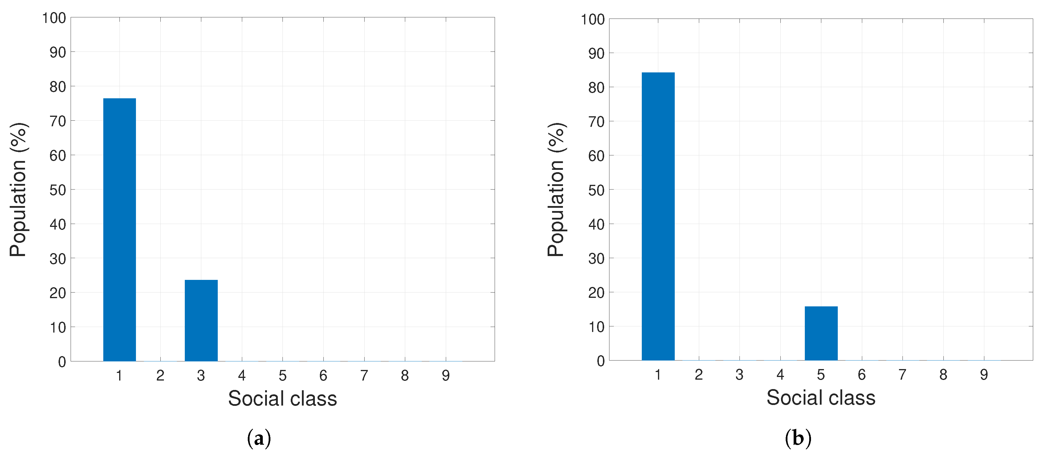
The asymptotic states of f shown in Figure 2a and Figure 2b correspond, respectively, to γ = 2 and γ = 4 . Notice that in the first case ( 1 , 3 ) S 0 and f i = 0 for i 1 , 3 , while in the second case ( 1 , 5 ) S 0 and f i = 0 for i 1 , 5 .
Even if finding explicit equilibria is a difficult task as clearly exposed in [15], one may look for some general features of equilibrium states. In particular, we wonder about the dependence of W (or V ) on parameters α and β . The following proposition shows that the asymptotic state does not depend on each single parameter value but on its quotient.
Proposition 2.
The asymptotic values W (for the constant population case r = 0 ) and V (for the general case) depend on α / β .
Searching equilibrium solutions of Equation (7) with r = 0 means looking for solutions of the system of algebraic equations f i = 0 , for i = 1 , , n . Then:
f i = k : ( i , k ) S 0 η i k f i f k + k : ( i , k ) S + ( 1 β ) η i k f i f k + k : ( i , k ) S ( 1 α ) η i k f i f k + k : ( i 1 , k ) S + β η i 1 , k f i 1 f k + k : ( i + 1 , k ) S α η i + 1 , k f i + 1 f k k = 1 n η i k f i f k .
The last term on the right hand side of (13) is equal to the positive contributions of the first three terms. Then:
f i = β k : ( i , k ) S + η i k f i f k + k : ( i 1 , k ) S + η i 1 , k f i 1 f k + α k : ( i , k ) S η i k f i f k + k : ( i + 1 , k ) S η i + 1 , k f i + 1 f k ,
which equals zero if:
k : ( i , k ) S + η i k f i f k + k : ( i 1 , k ) S + η i 1 , k f i 1 f k k : ( i , k ) S η i k f i f k k : ( i + 1 , k ) S η i + 1 , k f i + 1 f k = α β ,
showing that equilibrium points f i depends on the quotient α / β . Then, W = lim t i = 1 n u i f i ( t ) depends on α / β .
In the case r 0 , let us define f i ¯ f i N . Then:
f i N = f i N f i N · N N = f i N f i N · r = 1 N h = 1 n k = 1 n η h k B h k i f h f k f i k = 1 n η i k f k + r f i f i N · r = 1 N h = 1 n k = 1 n η h k B h k i f h f k f i k = 1 n η i k f k ,
where we used the derivative of a quotient, Equation (7) and the assumption that r i = r for i = 1 , , n . Proceeding as before in Equation (13), we get:
f i ¯ = 1 N β k : ( i , k ) S + η i k f i f k + k : ( i 1 , k ) S + η i 1 , k f i 1 f k + α k : ( i , k ) S η i k f i f k + k : ( i + 1 , k ) S η i + 1 , k f i + 1 f k ,
which again equals 0 if Equation (15) is satisfied. Thus, V = lim t i = 1 n u i f i ¯ also depends on α / β .
Figure 3 shows a numerical example of Proposition 2 for different combinations of α and β with the same value of α / β .

3.2. Measuring Inequality and the Gini Coefficient

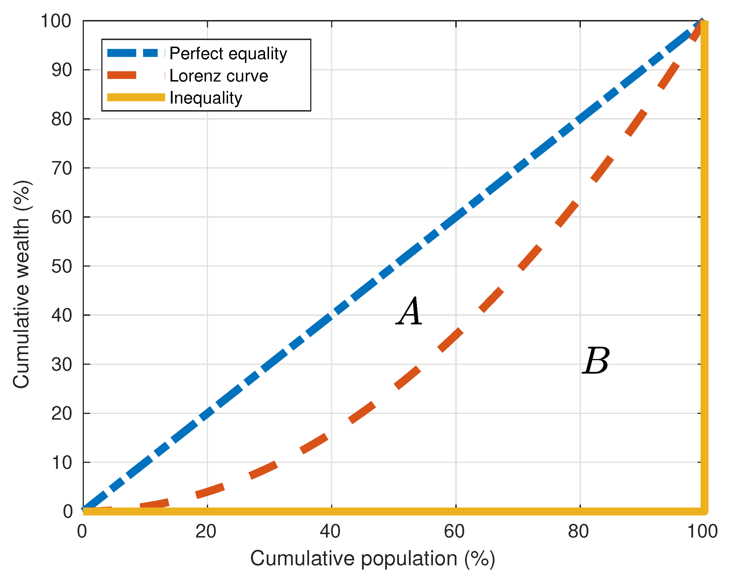
As already stated in Section 1, the Gini coefficient is one of the most universally used measures of inequality. It is usually defined in relation to the Lorenz curve, which plots the proportion of the total wealth of the population (vertical axis) that is cumulatively earned by the cumulative portion of the population (horizontal axis), see Figure 4. The line at 45 degrees thus represents perfect equality in the distribution of wealth. Let A be the area between the perfect equality (blue) and Lorenz (orange) curves, and B is the area under the Lorenz curve. It is then clear that A + B = 1 / 2 , which is the surface of the triangle with both perpendicular sides equal to 1. Then, g = A / ( A + B ) = A / ( 1 / 2 ) = 2 A , as shown in Figure 4. Since we are dealing with discrete activity values, we compute the Gini coefficient by using the trapezoid rule for computing the areas. A straightforward calculation yields:
g ( t ) = 1 2 i = 1 n 2 j = 1 i u j f j ( t ) u i f i ( t ) W ( t ) f i ( t ) N ( t ) ,
that let us obtain the Gini coefficient for each time t.
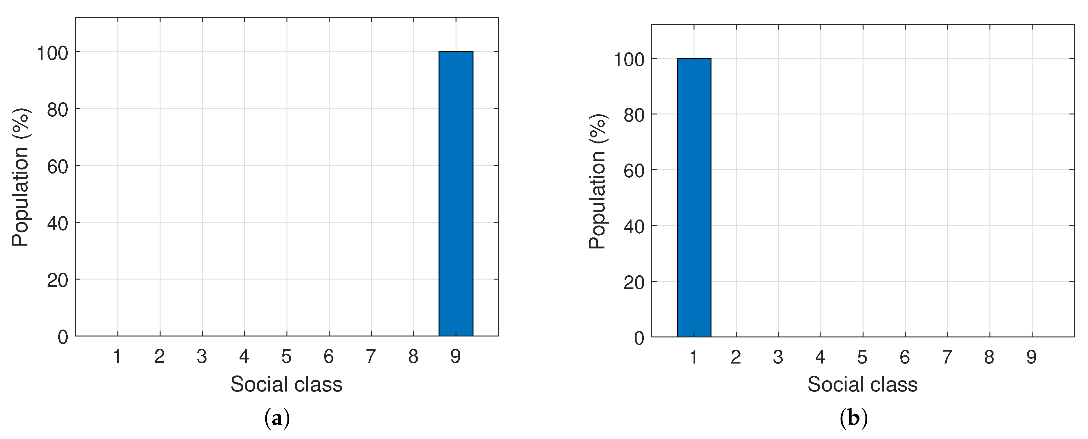
Please note that for instance, g = 0 can even correspond to a situation in which the whole population belongs to the highest social class or the lowest one, and thus a nation cannot be characterized only by g, but also by W, as shown in Figure 5 for the case of nine social classes.
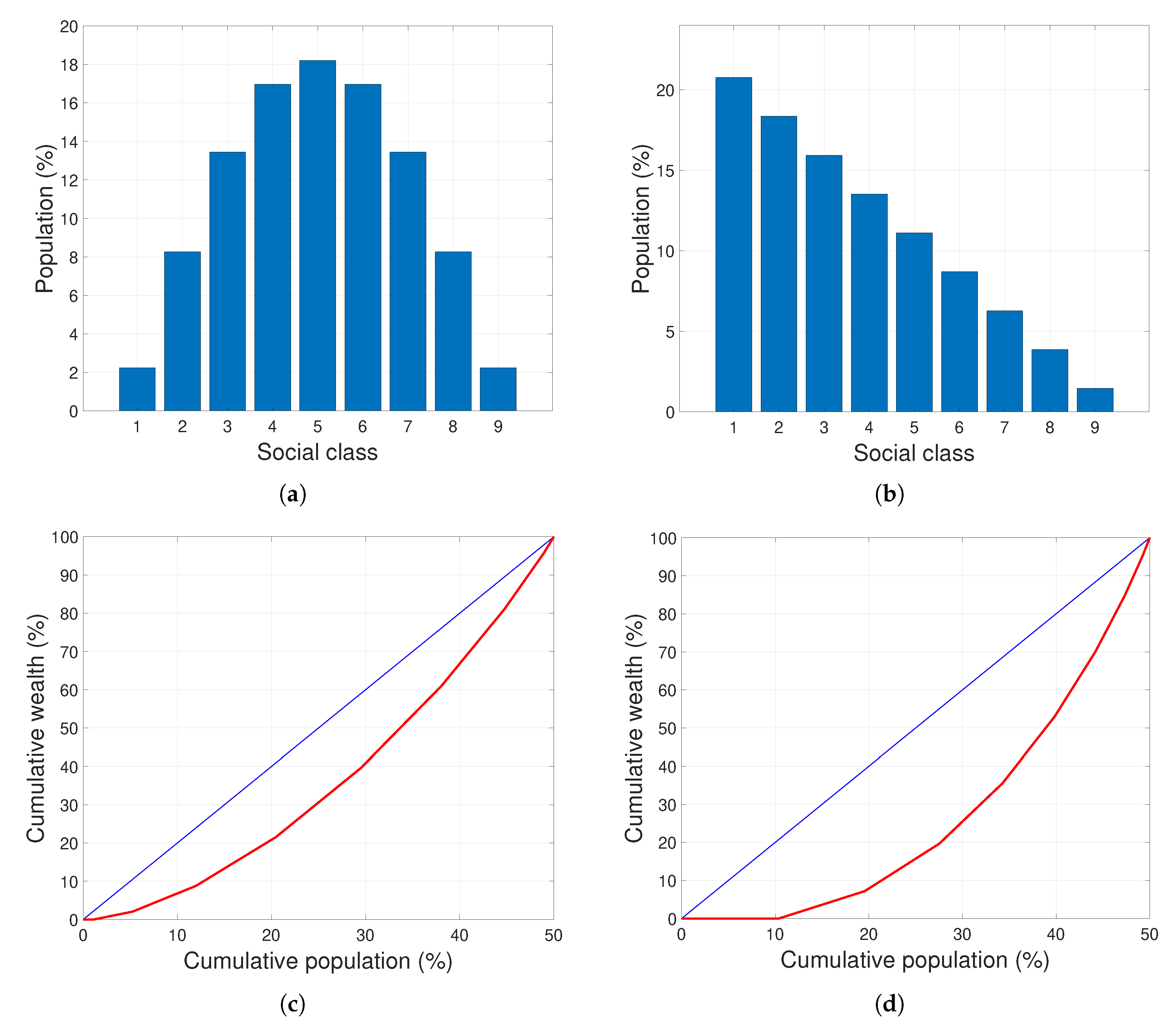
In the following, in order to perform a qualitative analysis of our model, we will consider two societies with n = 9 , I u = { u 1 = 0 , , u 9 = 1 } , and initial wealth distributions as shown in Figure 6a,b, and their corresponding Gini coefficients in Figure 6c,d. We will refer to these distributions as Society I and Society II. Society I has a symmetric distribution with respect to the middle class, being this class the dominant one. On the other hand, Society II is a more unequal society, with more people in lower classes than in higher classes. Both distributions are idealized.
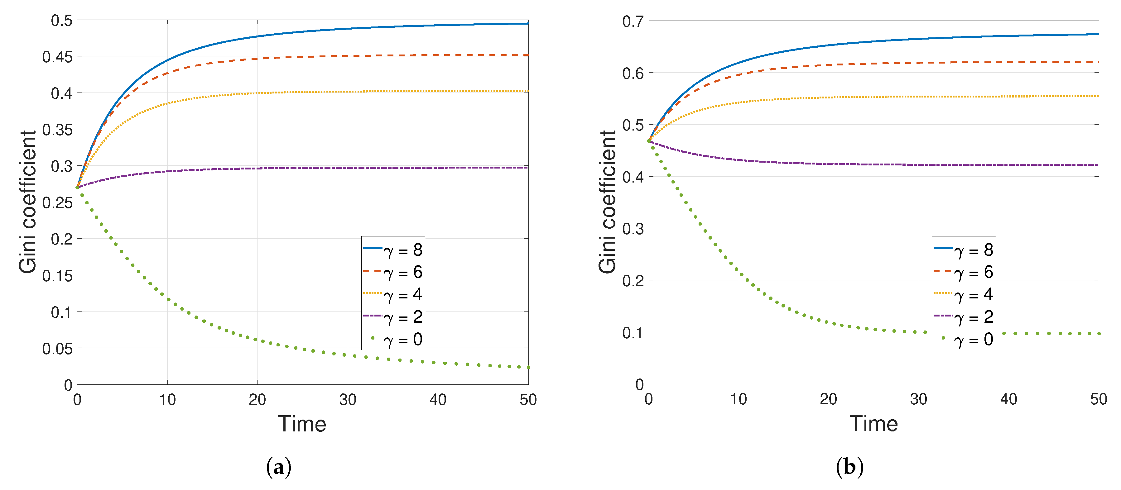
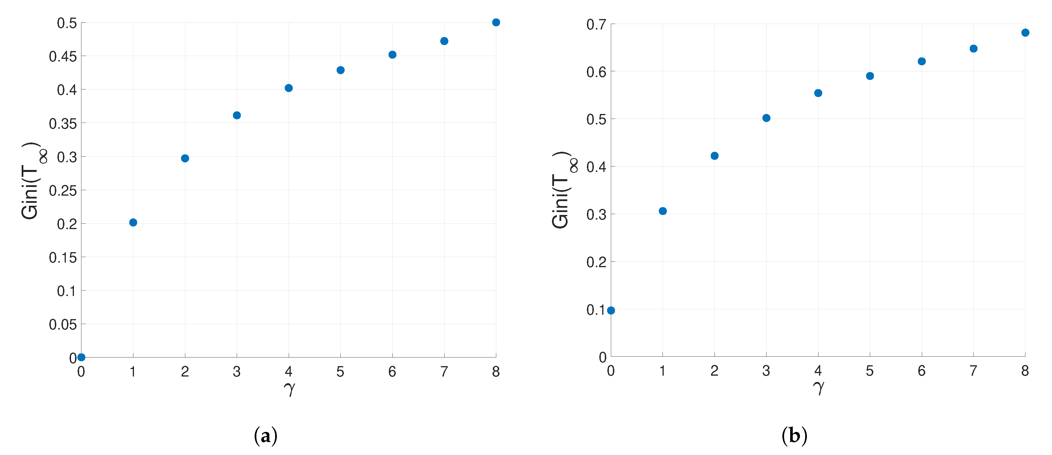
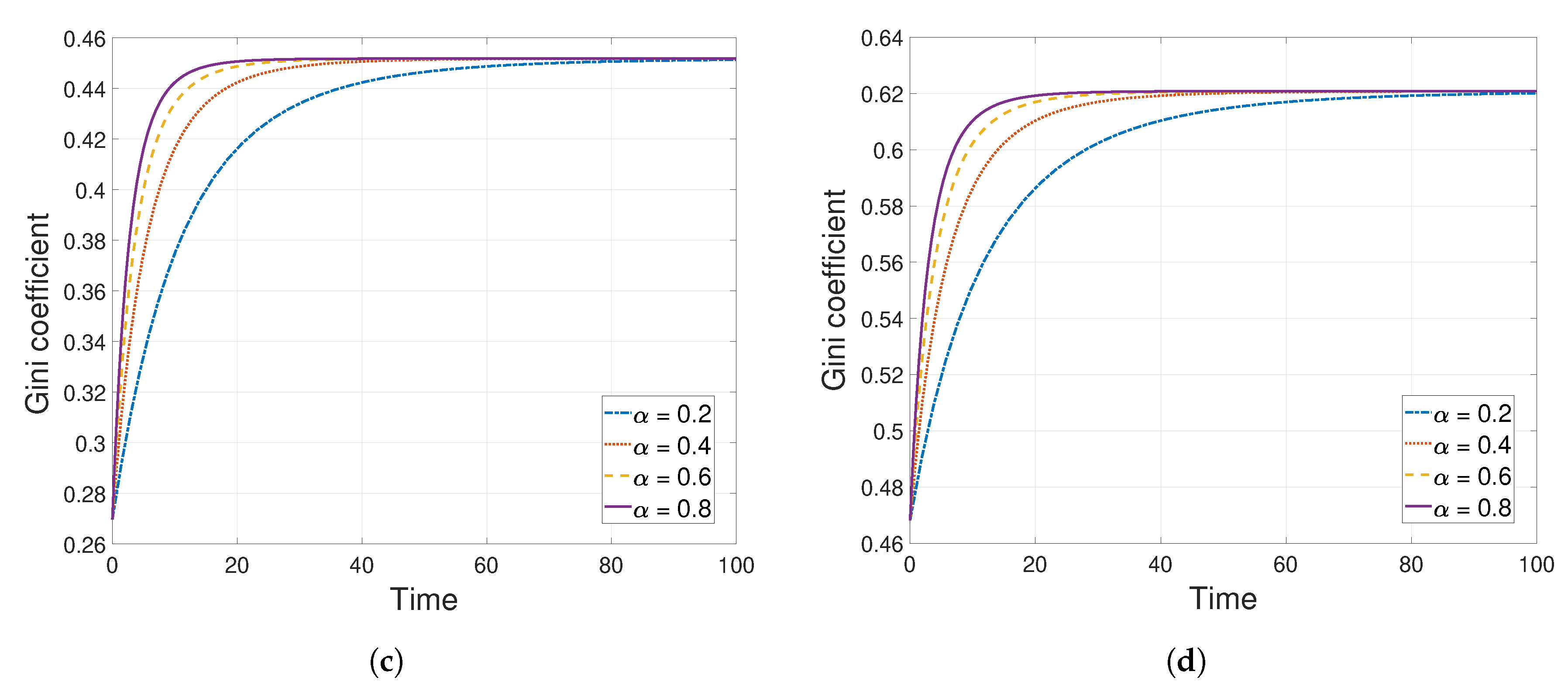
Let us firstly consider the simplest case r = 0 and α = β , which keeps the population and total wealth unchanging. Figure 7 shows the time evolution of the Gini coefficient in each society, for different choices of parameter γ , keeping α fixed and equal to 0.5. Notice that the monotonic behavior of g depends on the value of γ , since for small values of this parameter wealth tends to be more equally distributed (decreasing Gini). Figure 8 shows the Gini coefficient for a sufficiently large time in which the asymptotic state was already reached as a function of γ . Notice also that there is a clear correlation between the social threshold γ and the Gini coefficient g, confirming the fact that increasing values of the social threshold γ correspond to more unequal societies. In addition, if the probability of changing social state α is changed for fixed γ , neither the monotonic behavior nor the asymptotic states change, but it directly influences on how fast the Gini coefficient changes (the value of the derivative g ( t ) ), as shown in Figure 9.

4. Parameter Estimation from Empirical Data

This section is devoted to the model validation by studying its ability to reproduce and recover real data. In this sense, we would like to find the model parameters that best fit real data in terms of wealth distribution. If published data were available showing the percentages of the population belonging to each social class over time, we could seek the model parameters, described in Equation (7), which provide the wealth profiles ( f ) that best approximate those given by real data. If the aforementioned data were not explicitly available, an attempt could be made to approximate the total amount of wealth or the Gini coefficient of a certain society over time. Based on this reasoning, we will build the objective function and define an optimization problem.

4.1. Defining the Optimization Problem

Let N ( t ) , W ( t ) , f ( t ) and g ( t ) be total population, wealth, wealth distribution and Gini coefficient, respectively, in a given nation according to publicly available data. We will try to obtain the set of model parameters that best fit these data.
Firstly, notice that r is only associated with the total population and can thus be retrieved using only N ( t ) . Recall that N ( t ) = r N ( t ) , corresponding to an exponential model for population evolution. The proliferation rate r can thus be obtained in a first instance through the resolution of a least square problem.
To retrieve the other model parameters, let us write Equation (5) as an initial value problem:
f ( t ) = J f ( t ) , a , t [ 0 , T ] , f ( 0 ) = f 0 ,
where J = [ J 1 , , J n ] , emphasizing the dependence on the model parameters through the vector a = α , β , γ .
To find the set of parameters that best fit the available information W ( t ) , g ( t ) and f ( t ) , we define the objective function:
J ( a ) = ω 1 i = 1 n 0 T ( f i ( t ) f i ( t ) ) 2 d t + ω 2 0 T ( W ( t ) W ( t ) ) 2 d t + ω 3 0 T ( g ( t ) g ( t ) ) 2 d t = 0 T ω 1 f ( t ) f ( t ) 2 2 + ω 2 ( W ( t ) W ( t ) ) 2 + ω 3 ( g ( t ) g ( t ) ) 2 d t ,
with ω 1 , ω 2 and ω 3 non-negative weights. We pose the following optimization problem:
minimize a J ( a ) subject to f ( t ) = J f ( t ) , a , t [ 0 , T ] , f ( 0 ) = f 0 , a A ,
where the admissible set A = [ 0 , 1 ] × [ 0 , 1 ] × { 0 , , n 1 } lets the first two variables ( α , β ) be continuous, and the third one ( γ ) be integer.

4.2. Numerical Results

4.2.1. Case Study 1: Model Generated Data

Let us first consider the optimization problem given by Equation (19), in which f , W and g are generated by solving the direct problem (17), for a given choice of the model parameters. The idea of this test case is to investigate how close the original value of the parameter can be retrieved. However, this is not trivial, since it cannot be proved analytically if the optimization problem has a solution or, in that case, if it is unique.
In particular, in this case we firstly solve the direct problem with α = 0.4 , β = 0.3 (thus α / β = 4 / 3 ), γ = 4 and r = 0.01 with maximum time T = 50 years, with the two possible initial scenarios given by Society I and Society II in Figure 6. Since empirical measurements are often affected by perturbations, usually random ones, we add a Gaussian random noise to the solution of the direct problem. As stated in [30], it is in general valid to consider a 2% of Gaussian random noise for this kind of data. Consequently, we perform experiments adding to the solution 2%, 5% and 10% of random noise.
For both levels of noise, we perform several experiments for different combinations of weights in the objective function given by Equation (18), in order to test the quality and incidence of the information provided by each variable f , W and g . We then run each optimization problem 100 times for each case using different initial random parameter values (a), using a genetic algorithm that takes into account the mixed nature of the constraints as explained in [17]. Results are blue shown in Table 2, Table 3 and Table 4. For each experiment and initial wealth distribution, tables present the retrieved values of α , β , γ , α β , α / β and the relative error of the estimations. Notice that Experiments 1–3 correspond to a single non-zero weight in the objective function (18), while the others consider mixed combinations in which different magnitude order of weights is chosen to compensate the magnitude order of each term in Equation (18). Let us summarize the most relevant results:
  • In general, parameters are retrieved for data with 2 % noise with a lower relative error than in the case of 5 % and 10 % noise. However, notice that even with the highest level of noise we get reasonable results in most of the cases, so the results remain robust when we increase the noise.
  • The best possible situation would be to have available data on the distribution functions f . Indeed, the knowledge of these distributions allows also to calculate the Gini coefficient and wealth. That is why Experiments 1 and 6, which prioritize ω 1 , in general give good results.
  • When ω 1 0 or ω 3 0 , the parameter γ is recovered accurately. In contrast, the worst approximation is obtained in Experiment 2. Please note that it is reasonable to get these results due to the close relationship between γ and inequality, as explained in Section 3.2.
  • When wealth is prioritized over the complete profiles, i.e., larger values of ω 2 are considered, results lose accuracy and the quality of data recovery gets worse. Consequently, ω 2 should not be larger than the other weights. However, some countries may have available information only on total wealth or GDP and not on the complete social profiles. If this is the situation, availability of information on Gini coefficients can clearly improve the results, specifically γ : indeed, Experiments 7 and 8 get better results than Experiment 2.
  • It is worth noticing that in general, even if α and β are not retrieved accurately, their difference and quotient give much better results. This is expected from the detailed analysis performed in Section 3.1, where we showed that the dynamics depends on these quantities.

4.2.2. Case Study 2: US

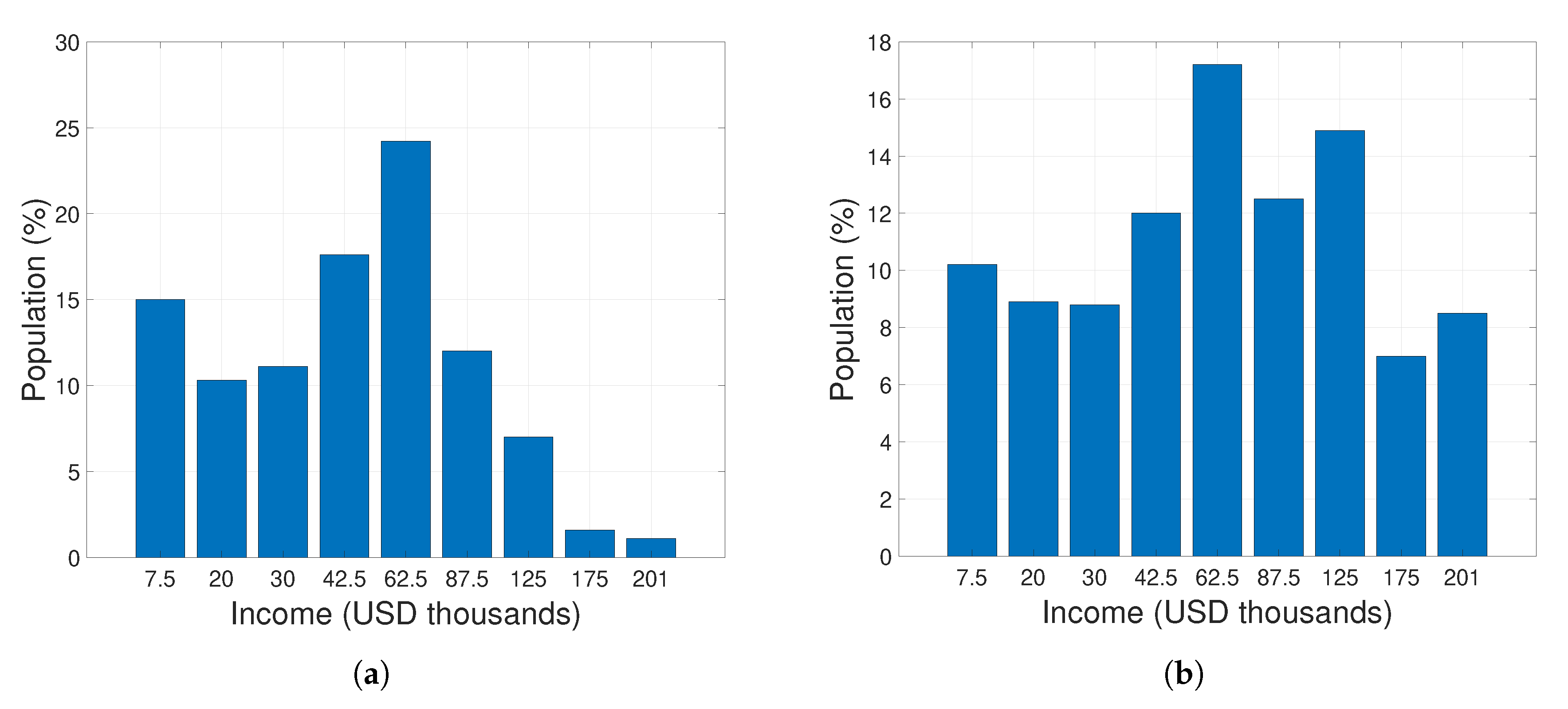
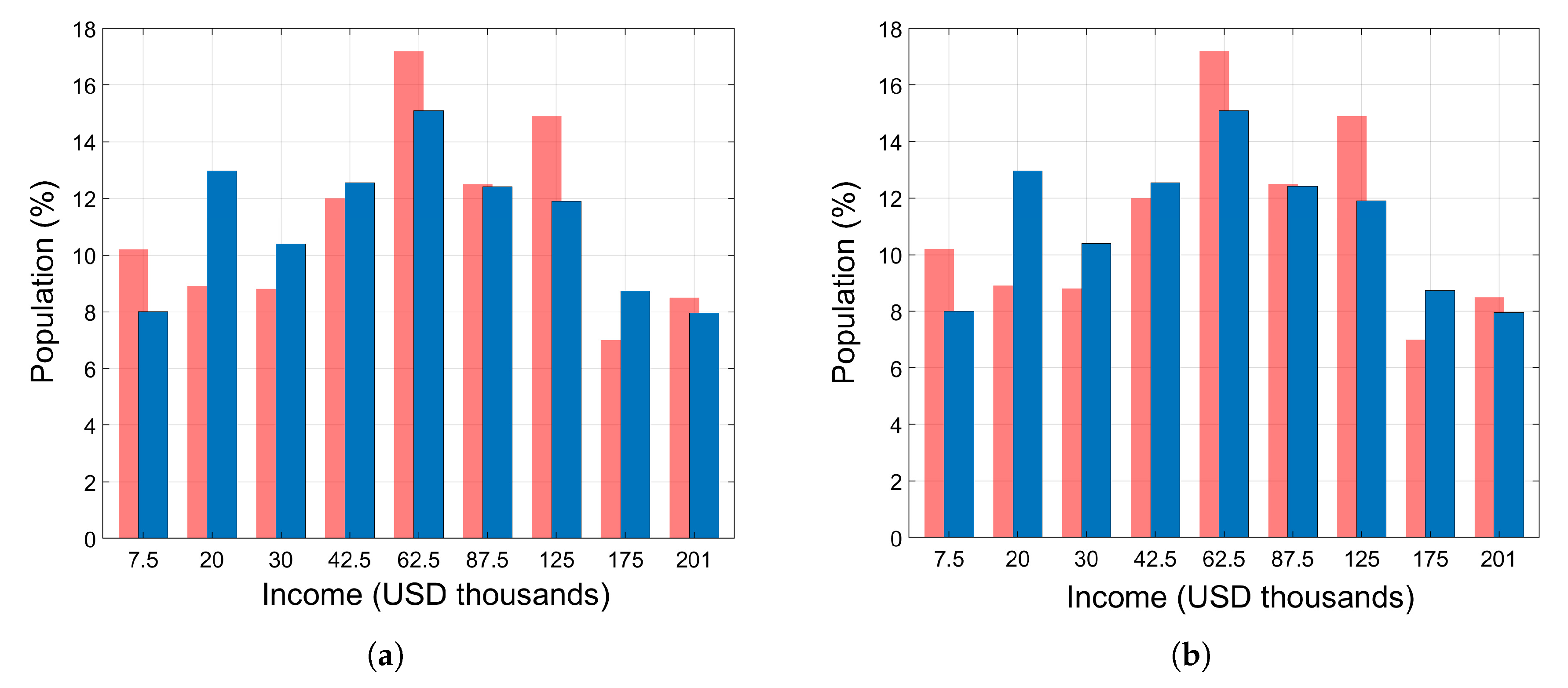
In this case study, we validate our model through the optimization technique for the case of the United States. A large amount of data is available for this country and, in particular, [31] provides the distribution of the population within social classes from 1967 to 2018. Social classes are characterized by income ranges, with a total of 9 intervals. In Figure 10a,b we show the distribution of the population in 1967 and 2018, respectively. The values of u i are chosen by taking the mean value of each interval.
That data, together with the total wealth and Gini coefficients for each year that can be straightforwardly computed, are inputs of our optimization problem. In this way, we choose the best two weight combinations in the objective function (18) to estimate the set of model parameters that best fit American data.
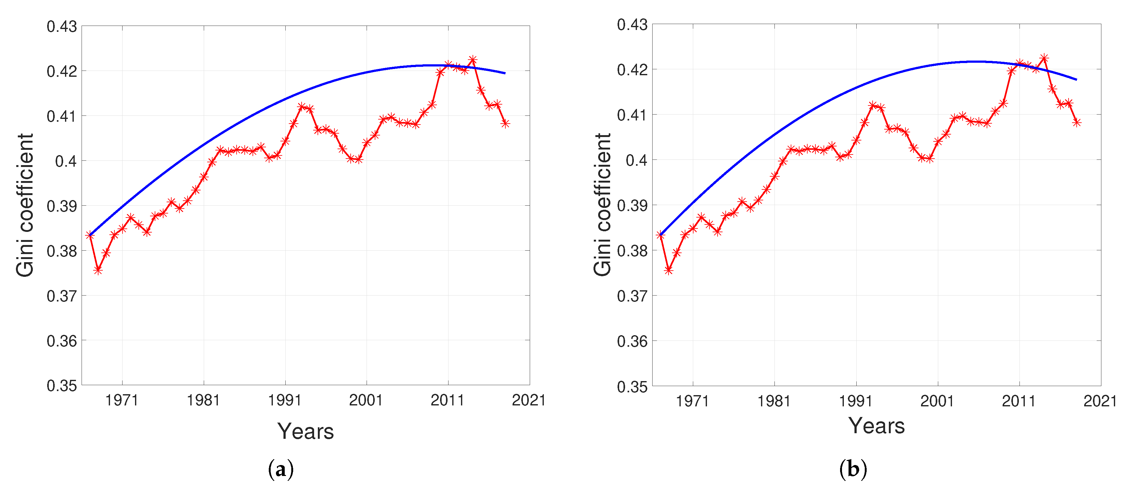
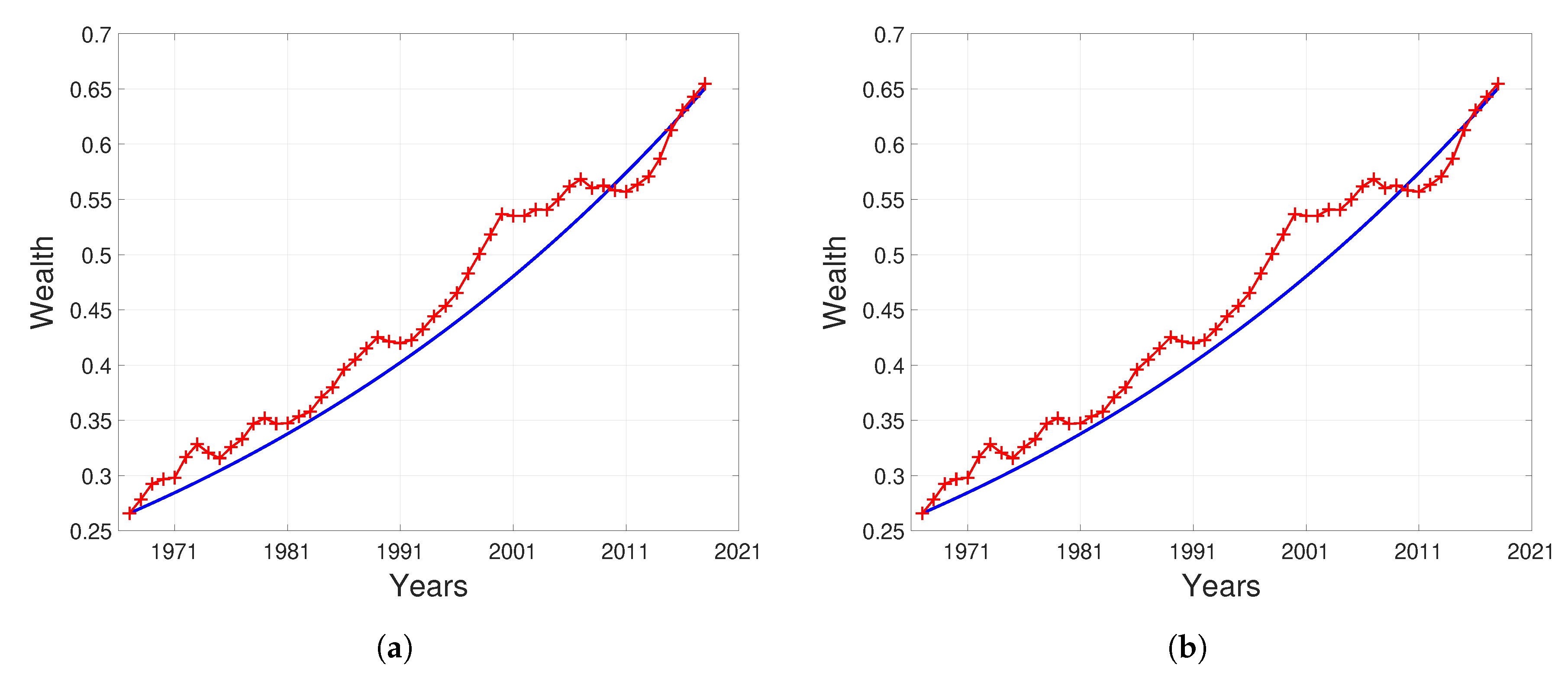
Figure 11a,b show the final distribution in 2018 for the two different choices of weights, comparing the real and simulated data. In addition, Figure 12 and Figure 13 show both the real and calculated Gini coefficient and wealth over time. Notice that US has a greater similarity to Society I than to Society II, since all classes, except the second one, respond to a pattern similar to Society I, with a predominant middle class.
Results are summarized in Table 5, where we show the retrieved parameter values. In both cases, the parameter α is lower than β confirming the fact that wealth shows an increasing trend in the long run for the US case. Notice that the obtained values for γ , together with the mean Gini coefficient for US (Figure 12), are in correspondence with the correlation observed in Figure 8a.

5. Conclusions and Looking Ahead

A kinetic model of wealth distribution in a society was presented in this paper, including two key aspects such as non-constant population and non-conservative trades. The qualitative analyses and numerical simulations show that the model is able to reproduce observed data and can thus be used by stakeholders for decision making. Even if an additional parameter ( β ) was introduced with respect to previous models [14,16,17], we showed that both α and β can be replaced by α / β in order to get useful information, without adding further complexity to the model.
The contents of the present paper let us individuate some perspectives for further research activity in the field. First of all, a deeper analytic study of social inequality can be performed. In particular, although the obtention of equilibrium points for the general case is a difficult task [15], it will be useful to study the qualitative behavior of the Gini coefficient from the perspective of dynamical systems, obtaining monotonic behaviors, bifurcation and tipping points. These results could even give some insight in the research of phenomena such as black swans [32]. A black swan is a highly improbable event with three principal characteristics: it is unpredictable, it carries a massive impact, and, after the fact, an explanation that makes it appear less random and more predictable than it was can be concocted.
Another additional topic worth of future analysis refers to space dynamics, which may be introduced through a network structure. This feature is also related to the macro-scale action in the various nodes of exogenous networks over individuals, as proposed in [10]. Dolfin et al. [9] also offers some useful hints by showing how the dynamics in a network enhances consensus. This structure can also be used to study the interaction between welfare dynamics and migration phenomena [1,33], aiming at better understanding the driving phenomena behind immigration, ways to curb, monitor and detect incoming flows and ways to help better adapt immigrants integrate into host societies.
Finally, some efforts must be addressed in the direction of the model implementation. In this sense, multidisciplinary collaborations are necessary to study the relationship between model parameters and concrete decision making processes by stakeholders.

Author Contributions

Conceptualization, B.A.B., D.K. and G.T.; Data curation, B.A.B., D.K. and G.T.; Formal analysis, B.A.B., D.K. and G.T.; Funding acquisition, B.A.B., D.K. and G.T.; Investigation, B.A.B., D.K. and G.T.; Methodology, B.A.B., D.K. and G.T.; Software, B.A.B., D.K. and G.T.; Visualization, B.A.B., D.K. and G.T.; Writing—original draft, B.A.B., D.K. and G.T.; Writing—review & editing, B.A.B., D.K. and G.T. All authors have read and agreed to the published version of the manuscript.

Funding

This research was funded by CONICET Grant Number PIP 11220150100500CO, Agencia Nacional de Promoción Científica y Tecnológica, Grant Number PICT 2015-1066, Secretaría de Ciencia y Técnica (UNC) and Secretaría General de Ciencia y Técnica (UNNE), Grant Number 19F010.

Conflicts of Interest

The authors declare no conflict of interest.

References

  1. Knopoff, D. On the modeling of migration phenomena on small networks. Math. Models Methods Appl. Sci. 2013, 23, 541–563. [Google Scholar] [CrossRef] [Green Version]
  2. UN General Assembly, International Migration and Development. Report of the Secretary-General, 18 May 2006, A/60/871. Available online: http://www.unhcr.org/refworld/docid/44ca2d934.html (accessed on 1 March 2020).
  3. Hurst, C.; Gibbon, H.; Nurse, A. Social Inequality: Forms, Causes, and Consequences; Routledge: Abington, UK, 2016. [Google Scholar]
  4. Yakovenko, V.; Rosser, J., Jr. Colloquium: Statistical mechanics of money, wealth, and income. Rev. Mod. Phys. 2009, 81, 1703. [Google Scholar] [CrossRef] [Green Version]
  5. Chakrabarti, B.; Chakraborti, A.; Chakravarty, S.; Chatterjee, A. Econophysics of Income and Wealth Distributions; Cambridge University Press: Cambridge, UK, 2013. [Google Scholar]
  6. Wolff, E.N. Household Wealth Trends in the United States, 1962 to 2013: What Happened over the Great Recession? RSF Russell Sage Found. J. Soc. Sci. 2016, 2, 24–43. [Google Scholar]
  7. Bellomo, N.; Knopoff, D.; Soler, J. On the difficult interplay between life “complexity” and mathematical sciences. Math. Models Methods Appl. Sci. 2013, 23, 1861–1913. [Google Scholar] [CrossRef]
  8. Bellomo, N. Modeling Complex Living Systems: A Kinetic Theory and Stochastic Game Approach; Springer Science & Business Media: Berlin/Heidelberg, Germany, 2008. [Google Scholar]
  9. Dolfin, M.; Lachowicz, M. Modeling opinion dynamics: How the network enhances consensus. Netw. Heterog. Media 2015, 4, 421–441. [Google Scholar] [CrossRef]
  10. Knopoff, D. On a mathematical theory of complex systems on networks with application to opinion formation. Math. Models Methods Appl. Sci. 2014, 24, 405–426. [Google Scholar] [CrossRef]
  11. Burini, D.; De Lillo, S. On the complex interaction between collective learning and social dynamics. Symmetry 2019, 11, 967. [Google Scholar] [CrossRef] [Green Version]
  12. Burini, D.; De Lillo, S.; Gibelli, L. Collective learning modeling based on the kinetic theory of active particles. Phys. Life Rev. 2016, 16, 126–139. [Google Scholar] [CrossRef]
  13. Dolfin, M.; Knopoff, D.; Leonida, L.; Patti, D. Escaping the trap of “blocking”: A kinetic model linking economic development and political competition. Kinet. Relat. Models 2017, 10, 423–443. [Google Scholar] [CrossRef]
  14. Bertotti, M.L.; Delitala, M. From discrete kinetic and stochastic game theory to modelling complex systems in applied sciences. Math. Models Methods Appl. Sci. 2004, 14, 1061–1084. [Google Scholar] [CrossRef]
  15. Bertotti, M.L.; Delitala, M. Conservation laws and asymptotic behavior of a model of social dynamics. Nonlinear Anal. RWA 2008, 9, 183–196. [Google Scholar] [CrossRef]
  16. Bellomo, N.; Herrero, M.A.; Tosin, A. On the dynamics of social conflicts looking for the Black Swan. Kinet. Relat. Models 2013, 6, 459–479. [Google Scholar] [CrossRef] [Green Version]
  17. Knopoff, D.; Torres, G. On an optimal control strategy in a kinetic social dynamics model. Commun. Appl. Ind. Math. 2018, 9, 22–33. [Google Scholar] [CrossRef] [Green Version]
  18. Furioli, G.; Pulvirenti, A.; Terraneo, E.; Toscani, G. Fokker–Planck equations in the modeling of socio–economic phenomena. Math. Models Methods Appl. Sci. 2017, 27, 115–158. [Google Scholar] [CrossRef] [Green Version]
  19. Furioli, G.; Pulvirenti, A.; Terraneo, E.; Toscani, G. Non–Maxwellian kinetic equations modeling the dynamics of wealth distribution. Math. Models Methods Appl. Sci. 2020, 30, 1–41. [Google Scholar] [CrossRef]
  20. Lim, G.; Min, S. Analysis of solidarity effect for entropy, Pareto, and Gini indices on two-class society using kinetic wealth exchange model. Entropy 2020, 22, 386. [Google Scholar] [CrossRef] [Green Version]
  21. Quadrini, V.; Rios-Rull, J. Models of the distribution of wealth. Fed. Reserve Bank Minneap. Q. Rev. 1997, 21, 1–21. [Google Scholar]
  22. De Nardi, M.; Fella, G. Saving and wealth inequality. Rev. Econ. Dyn. 2017, 26, 280–300. [Google Scholar] [CrossRef]
  23. Schelling, T. Dynamic models of segregation. J. Math. Sociol. 1971, 1, 143–186. [Google Scholar] [CrossRef]
  24. Benard, S.; Willer, R. A wealth and status-based model of residential segregation. Math. Sociol. 2007, 31, 149–174. [Google Scholar] [CrossRef]
  25. Hatna, E.; Benenson, I. The Schelling model of ethnic residential dynamics: Beyond the integrated-segregated dichotomy of patterns. J. Artif. Soc. Soc. Simul. 2012, 15, 6. [Google Scholar] [CrossRef]
  26. Hazan, A.; Randon-Furling, J. A Schelling model with switching agents: Decreasing segregation via random allocation and social mobility. Eur. Phys. J. B 2013, 86, 421. [Google Scholar] [CrossRef]
  27. Chuang, Y.; Chou, T.; D’Orsogna, M. A network model of immigration: Enclave formation vs. cultural integration. Netw. Heterog. Media 2019, 14, 53. [Google Scholar] [CrossRef] [Green Version]
  28. Jarvis, M.; Lange, G.M.; Hamilton, K.; Desai, D.; Fraumeni, B.; Edens, B.; Ferreira, S.; Fraumeni, B.; Jarvis, M.; Kingsmill, W.; et al. The Changing Wealth of Nations: Measuring Sustainable Development in the New Millennium; The World Bank: Washington, DC, USA, 2011. [Google Scholar]
  29. Cohen, J.E. Population growth and earth’s human carrying capacity. Science 1995, 269, 341–346. [Google Scholar] [CrossRef] [Green Version]
  30. Guzman, G.G. Household Income; American Community Survey Briefs: Washington, DC, USA, 2016. [Google Scholar]
  31. United States Census Bureau. Available online: https://www.census.gov/en.html (accessed on 1 March 2020).
  32. Taleb, N.N. The Black Swan: The Impact of the Highly Improbable; Random House: New York, NY, USA, 2007. [Google Scholar]
  33. Chuang, Y.L.; Chou, T.; D’Orsogna, M.R. Age-structured social interactions enhance radicalization. J. Math. Sociol. 2018, 3, 128–151. [Google Scholar] [CrossRef] [Green Version]
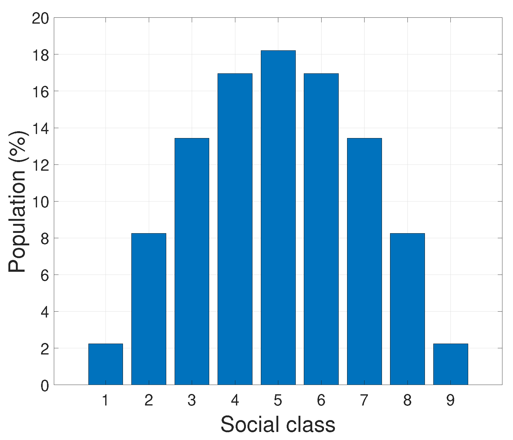
Figure 1. Initial distribution of a population.
Mathematics 08 00786 g001
Figure 2. Simulated equilibrium states for the society with the initial distribution shown in Figure 1. Simulations are run for α = 0.4 , β = 0.1 , r = 0.01 and (a) γ = 2 (b) γ = 4 , until the asymptotic states are reached.
Mathematics 08 00786 g002
Figure 3. Asymptotic values of (a) wealth and (b) wealth per capita for the system with initial condition shown in Figure 1, with r = 0.01 , γ = 4 and three different combinations of α and β such that α / β = 4 .
Mathematics 08 00786 g003
Figure 4. Graphical representation of the Gini coefficient. A is the area between the Lorenz and perfect equality curves, B is the area between the Lorenz and inequality curves, and the Gini coefficient is computed by A / ( A + B ) .
Mathematics 08 00786 g004
Figure 5. Two possible wealth distributions within a society. In (a) the whole population belongs to the highest social class, while in (b) the whole population belongs to the lowest one. However, g = 0 in both cases.
Mathematics 08 00786 g005
Figure 6. Wealth distribution, at t = 0 , for (a) Society I, and (b) for Society II. Gini coefficient, at t = 0 , for (c) Society I, and (d) for Society II.
Mathematics 08 00786 g006
Figure 7. Temporal evolution (in years) of the Gini coefficient for different values of γ , with α = 0.5 fixed, for (a) Society I, and (b) for Society II.
Mathematics 08 00786 g007
Figure 8. Asymptotic value of the Gini coefficient as a function of γ , with α = 0.5 fixed, for (a) Society I, and (b) Society II.
Mathematics 08 00786 g008
Figure 9. Temporal evolution (in years) of Gini coefficient for several cases. (a) Society I, γ = 2 ; (b) Society II, γ = 2 ; (c) Society I, γ = 6 ; (d) Society II, γ = 6 .
Mathematics 08 00786 g009aMathematics 08 00786 g009b
Figure 10. Distribution of annual income in the US in (a) 1967 and (b) 2018 according to publicly available data.
Mathematics 08 00786 g010
Figure 11. Simulated outputs of distribution of annual income in 2018 using (a) ω 1 = 1 and ω 2 = ω 3 = 0 and (b) ω 1 = 10 , ω 2 = 100 , ω 3 = 10 . Left red bars represent real data, while right blue bars correspond to simulated results.
Mathematics 08 00786 g011
Figure 12. Simulated outputs for Gini coefficent (continuous line) versus real Gini coefficient (*) using (a) ω 1 = 1 and ω 2 = ω 3 = 0 and (b) ω 1 = 10 , ω 2 = 100 , ω 3 = 10 .
Mathematics 08 00786 g012
Figure 13. Simulated outputs for wealth (continuous line) versus real Wealth (+) using (a) ω 1 = 1 and ω 2 = ω 3 = 0 and (b) ω 1 = 10 , ω 2 = 100 , ω 3 = 10 .
Mathematics 08 00786 g013
Table 1. List of symbols.
SymbolDescription
nNumber of social classes
u i , i = 1 , , n Social states
f i , i = 1 , , n Number of individuals that have social state u i
TMaximum observation time
NPopulation
WTotal wealth
VWealth per capita
η h k , h , k = 1 , , n Encounter rates
B h k i , h , k , i = 1 , , n Transition probability densities
r i , i = 1 , , n , rNet proliferation rates
γ Social threshold
α Probability of decreasing one social class
β Probability of increasing one social class
W Asymptotic value of W when t
V Asymptotic value of V when t
f i Asymptotic value of f i when t
gGini coefficient
Table 2. Generated data with noise 2 % .
Experiment Society I E ( % ) Society II E ( % )
α 0.4099 2.48 0.4306 7.65
ω 1 = 1 β 0.3088 2.93 0.3292 9.73
1 ω 2 = 0 γ 4.0000 0.00 4.0000 0.00
ω 3 = 0 α / β 1.3274 0.45 1.3080 1.90
β α 0.1011 1.10 0.1014 1.40
α 0.5688 42.20 0.5440 36.00
ω 1 = 0 β 0.4372 45.73 0.4141 38.03
2 ω 2 = 1 γ 5.3000 32.50 5.2400 31.00
ω 3 = 0 α / β 1.3010 2.43 1.3137 1.47
β α 0.1316 31.60 0.1299 29.90
α 0.4391 9.78 0.4296 7.40
ω 1 = 0 β 0.3425 14.17 0.3327 10.90
3 ω 2 = 0 γ 4.3800 9.50 4.3600 9.00
ω 3 = 1 α / β 1.2820 3.85 1.2913 3.16
β α 0.0966 3.40 0.0969 3.10
α 0.4359 8.98 0.4564 14.10
ω 1 = 10 β 0.3347 11.57 0.3551 18.37
4 ω 2 = 100 γ 4.0000 0.00 4.0000 0.00
ω 3 = 10 α / β 1.3024 2.32 1.2853 3.60
β α 0.1012 1.20 0.1013 1.30
α 0.4521 13.03 0.4382 9.55
ω 1 = 10 β 0.3509 16.97 0.3370 12.33
5 ω 2 = 100 γ 4.0000 0.00 4.0000 0.00
ω 3 = 0 α / β 1.2884 3.37 1.3003 2.48
β α 0.1012 1.20 0.1012 1.20
α 0.3973 0.68 0.4030 0.75
ω 1 = 10 β 0.2963 1.23 0.3019 0.63
6 ω 2 = 0 γ 4.0000 0.00 4.0000 0.00
ω 3 = 1 α / β 1.3409 0.57 1.3349 0.12
β α 0.1010 1.00 0.1011 1.10
α 0.4978 24.45 0.5070 26.75
ω 1 = 0 β 0.3955 31.83 0.4048 34.93
7 ω 2 = 10 γ 4.1000 2.50 4.0800 2.00
ω 3 = 1 α / β 1.2587 5.60 1.2525 6.07
β α 0.1023 2.30 0.1022 2.20
α 0.4928 23.20 0.5080 27.00
ω 1 = 0 β 0.3918 30.60 0.4070 35.67
8 ω 2 = 1 γ 4.0200 0.50 4.0600 1.50
ω 3 = 10 α / β 1.2578 5.67 1.2482 6.39
β α 0.1010 1.00 0.1010 1.00
Table 3. Generated data with noise 5 % .
Experiment Society I E ( % ) Society II E ( % )
α 0.4120 3.00 0.4102 2.55
ω 1 = 1 β 0.3108 3.60 0.3091 3.03
1 ω 2 = 0 γ 4.0000 0.00 4.0000 0.00
ω 3 = 0 α / β 1.3256 0.58 1.3271 0.47
β α 0.1012 1.20 0.1011 1.10
α 0.5708 42.70 0.5828 45.70
ω 1 = 0 β 0.4396 46.53 0.4485 49.50
2 ω 2 = 1 γ 5.2700 31.75 5.4000 35.00
ω 3 = 0 α / β 1.2985 2.62 1.2994 2.54
β α 0.1312 31.20 0.1343 34.30
α 0.4252 6.30 0.4321 8.03
ω 1 = 0 β 0.3301 10.03 0.3359 11.97
3 ω 2 = 0 γ 4.5500 13.75 4.4300 10.75
ω 3 = 1 α / β 1.2881 3.39 1.2864 3.52
β α 0.0951 4.90 0.0962 3.80
α 0.4266 6.65 0.4453 11.33
ω 1 = 10 β 0.3254 8.47 0.3440 14.67
4 ω 2 = 100 γ 4.0000 0.00 4.0000 0.00
ω 3 = 10 α / β 1.3108 1.69 1.2943 2.93
β α 0.1012 1.20 0.1013 1.30
α 0.4563 14.08 0.4290 7.25
ω 1 = 10 β 0.3550 18.33 0.3279 9.30
5 ω 2 = 100 γ 4.0000 0.00 4.0000 0.00
ω 3 = 0 α / β 1.2854 3.60 1.3083 1.86
β α 0.1013 1.30 0.1011 1.10
α 0.3972 0.70 0.3970 0.75
ω 1 = 10 β 0.2966 1.13 0.2959 1.37
6 ω 2 = 0 γ 4.0000 0.00 4.0000 0.00
ω 3 = 1 α / β 1.3392 0.44 1.3417 0.63
β α 0.1006 0.60 0.1011 1.10
α 0.5089 27.23 0.5022 25.55
ω 1 = 0 β 0.4065 35.50 0.4004 33.47
7 ω 2 = 10 γ 4.1100 2.75 4.0500 1.25
ω 3 = 1 α / β 1.2519 6.11 1.2542 5.93
β α 0.1024 2.40 0.1018 1.80
α 0.4726 18.15 0.4915 22.88
ω 1 = 0 β 0.3717 23.90 0.3907 30.23
8 ω 2 = 1 γ 4.0700 1.75 4.0900 2.25
ω 3 = 10 α / β 1.2715 4.64 1.2580 5.65
β α 0.1009 0.90 0.1008 0.80
Table 4. Generated data with noise 10 % .
Experiment Society I E ( % ) Society II E ( % )
α 0.4344 8.60 0.4069 1.73
ω 1 = 1 β 0.3293 9.77 0.2978 0.73
1 ω 2 = 0 γ 4.0000 0.00 4.0000 0.00
ω 3 = 0 α / β 1.3191 1.07 1.3663 2.47
β α 0.1051 5.09 0.1091 9.09
α 0.5210 30.25 0.4872 21.81
ω 1 = 0 β 0.4177 39.23 0.3259 8.62
2 ω 2 = 1 γ 4.2000 5.00 5.5000 37.50
ω 3 = 0 α / β 1.2474 6.45 1.4952 12.14
β α 0.1033 3.33 0.1614 61.38
α 0.4294 7.34 0.3002 24.95
ω 1 = 0 β 0.3297 9.89 0.2016 32.81
3 ω 2 = 0 γ 4.2000 5.00 4.6000 15.00
ω 3 = 1 α / β 1.3024 2.32 1.4894 11.70
β α 0.0997 0.31 0.0986 1.36
α 0.4764 19.10 0.4140 3.49
ω 1 = 10 β 0.3762 25.39 0.3031 1.03
4 ω 2 = 100 γ 4.0000 0.00 4.0000 0.00
ω 3 = 10 α / β 1.2665 5.01 1.3658 2.44
β α 0.1002 0.25 0.1109 10.87
α 0.4272 6.79 0.4141 3.53
ω 1 = 10 β 0.3274 9.14 0.3033 1.09
5 ω 2 = 100 γ 4.0000 0.00 4.0000 0.00
ω 3 = 0 α / β 1.3047 2.15 1.3655 2.42
β α 0.0998 0.24 0.1109 10.86
α 0.4328 8.20 0.4101 2.53
ω 1 = 10 β 0.3278 9.26 0.3009 0.28
6 ω 2 = 0 γ 4.0000 0.00 4.0000 0.00
ω 3 = 1 α / β 1.3204 0.97 1.3632 2.24
β α 0.1050 5.02 0.1093 9.28
α 0.5896 47.40 0.4514 12.86
ω 1 = 0 β 0.4884 62.81 0.3382 12.75
7 ω 2 = 10 γ 4.1000 2.50 4.1000 2.50
ω 3 = 1 α / β 1.2071 9.47 1.3346 0.10
β α 0.1012 1.17 0.1132 13.19
α 0.4215 5.38 0.3851 3.73
ω 1 = 0 β 0.3213 7.10 0.2739 8.70
8 ω 2 = 1 γ 4.2000 5.00 4.1000 2.50
ω 3 = 10 α / β 1.3120 1.60 1.4060 5.45
β α 0.1002 0.23 0.1112 11.19
Table 5. Results for US data.
α 0.0012
ω 1 = 1 β 0.0448
ω 2 = 0 γ 4.000
ω 3 = 0 α / β 0.0272
β α 0.0435
α 0.0017
ω 1 = 10 β 0.0502
ω 2 = 100 γ 4.000
ω 3 = 10 α / β 0.0344
β α 0.0485