Article

Multiobjective Model Predictive Control of a Parabolic Advection-Diffusion-Reaction Equation

1
Department of Mathematics and Statistics, University of Konstanz, D-78457 Konstanz, Germany;
2
Mathematical Institute, University of Bayreuth, D-95440 Bayreuth, Germany
*
Authors to whom correspondence should be addressed.
Mathematics 2020, 8(5), 777; https://doi.org/10.3390/math8050777
Submission received: 9 March 2020 / Revised: 9 April 2020 / Accepted: 28 April 2020 / Published: 12 May 2020
(This article belongs to the Special Issue Recent Trends in Multiobjective Optimization and Optimal Control)

Abstract

:
In the present paper, a multiobjective optimal control problem governed by a linear parabolic advection-diffusion-reaction equation is considered. The optimal controls are computed by applying model predictive control (MPC), which is a method for controlling dynamical systems over long or infinite time horizons by successively computing optimal controls over a moving finite time horizon. Numerical experiments illustrate that the proposed solution approach can be successfully applied although some of the assumptions which are necessary to conduct the theoretical analysis cannot be guaranteed for the studied tests.

1. Introduction

Model predictive control (MPC) is a method for controlling dynamical systems over long or infinite time horizons by successively computing optimal controls over a moving finite time horizon; cf., for example, Reference [1]. The successive re-optimization on the one hand introduces a feedback mechanism, which makes the method attractive as a real-time control scheme and as such it is widely used in industry [2]. On the other hand, MPC provides a method to reduce the complexity of optimal control problems by splitting up problems on long or infinite horizons into smaller subproblems over shorter horizons. As such, MPC can be seen as a model reduction technique in time. Clearly, this approach only makes sense if the solution generated by MPC is in some sense close to the true optimal solution. Fortunately, this approximate optimality property can be rigorously proved for many classes of optimal control problems, see, for example, References [3,4] and the references therein.
In practice, it is often the case that a single optimization criterion is not sufficient for modelling the demands in a given application. This leads to the concept of multiobjective optimal control, in which typically there does not exist a single optimal value but rather a whole set of optimal values, the so called Pareto front. Due to its usefulness in practice it is no surprise that this concept has been used and investigated also in the MPC context, see, for example, References [5,6,7,8,9]. Particularly, in References [10,11] MPC algorithms were presented that allow for rigorous suboptimality estimates also in the multiobjective case. The main feature of this class of algorithms is a particular constraint that depends on the chosen point on the Pareto front when solving the first optimal control problem in the MPC scheme and that is applied in all subsequent optimal control problems. While the examples in References [10,11] are limited to finite dimensional systems, in this paper we show that this idea can be successfully applied also to optimal control problems governed by partial differential equations (PDEs) and that the necessary constraint can be efficiently implemented using a gradient descent scheme. While we will see that some of the assumptions made in References [10,11] are difficult to satisfy for PDE governed problems, our numerical tests will show that the algorithm nevertheless performs very well.
In the literature there is a vast amount of methods for multiobjectice optimization; see for example, References [12,13]. However, in the context of PDE constrained problems there are only a few papers available. We refer, for example, to References [14,15,16,17,18]. In this paper, for computing the Pareto set and/or the Pareto front of the multiobjective optimal control problem (MOCP) we use the Euclidean reference point method, which was introduced in References [19,20] and already used for solving multiobjective optimal control problems with two cost functions in References [21,22,23].
The paper is organized as follows: In Section 2 we pose the multiobjective optimal control problem (MOCP). The algorithmic approach for multiobjectice model predictive control (MOMPC) is explained and analyzed in Section 3. Numerical experiments are presented in Section 4. In the last section we draw a few conclusions.

2. The Multiobjective Optimal Control Problem

Let Ω R 2 be a bounded domain with Lipschitz-continuous boundary Γ = Ω , T > 0 , Q = ( 0 , T ) × Ω , Σ = ( 0 , T ) × Γ . Given an initial condition y L 2 ( Ω ) we consider the following parametrized parabolic advection-diffusion-reaction equation with the diffusion coefficient d > 0 , the advection field c L ( ( 0 , T ) × Ω ; R 2 ) and the reaction coefficient r 0 :
y t ( t , x ) d Δ y ( t , x ) + c ( t , x ) · y ( t , x ) + r y ( t , x ) = 0 a . e .   i n   Q , d y n ( t , x ) = i = 1 m u i ( t ) b i ( x ) a . e .   o n   Σ , y ( 0 , x ) = y ( x ) a . e .   i n   Ω .
The functions b i L ( Γ ) , 1 i m , denote given control shape functions, for example, characteristic functions:
Γ = i = 1 m Γ i , b i ( s ) = χ Γ i ( s ) , 1 i m , b i L 2 ( Γ ) 2 = | Γ i | .
By setting H = L 2 ( Ω ) and V = H 1 ( Ω ) , one can show that (1) has a unique weak solution y = y ( u , y ) W ( 0 , T ) = H 1 ( 0 , T ; V ) L 2 ( 0 , T ; V ) for all controls u L 2 ( 0 , T ; R m ) = : U and all initial conditions y H . Recall that W ( 0 , T ) is a Hilbert space endowed with its common inner product. Moreover, W ( 0 , T ) is continuously embedded into C ( [ 0 , T ] ; H ) ; cf. Reference [24]. The solution operator S : U × H W ( 0 , T ) L 2 ( 0 , T ; H ) , which maps any control u U and initial value y H to the solution y = S ( u , y ) of (1), is affine linear and continuous in both components.
Given a fixed initial value y H the multiobjective optimal control problem (MOCP) reads
min u U J ^ ( u , y ) = min u U J ^ 1 ( u , y ) J ^ 2 ( u , y ) ,
where the two objectives J ^ 1 , J ^ 2 : U × H R are given by
J ^ i ( u , y ) : = σ i 1 2 C i 1 S ( u , y ) y i 1 L 2 ( 0 , T ; H ) 2 + σ i 2 2 C i 2 S ( u , y ) ( T ) y i 2 H 2 + σ i 3 2 u L 2 ( 0 , T ; R m ) 2
for nonnegative weighting parameters σ i 1 , σ i 2 , σ i 3 with σ i 1 + σ i 2 + σ i 3 > 0 , linear mappings C i 1 L ( L 2 ( 0 , T ; H ) ) and C i 2 L ( H ) and desired states y i 1 L 2 ( 0 , T ; H ) and y i 2 H for i = 1 , 2 . Here, for example, L ( L 2 ( 0 , T ; H ) ) denotes the Banach space of all linear and bounded operators mapping from L 2 ( 0 , T ; H ) into itself.
Problem (MOCP) involves the minimization of a vector-valued objective J ^ ( · , y ) : U R 2 . This is done by using the concept of Pareto optimality; see, for example, Reference [12].
Definition 1.
The point u ¯ U is called Pareto optimal for (MOCP), if there is no other control u U with J ^ i ( u , y ) J ^ i ( u ¯ , y ) for i = 1 , 2 and J ^ l ( u , y ) < J ^ l ( u ¯ , y ) for at least one l { 1 , 2 } . The set
U o p t ( y ) = { u U u i s P a r e t o o p t i m a l }
is called the Pareto set, and
J o p t ( y ) = J ^ ( U o p t , y )
is called the Pareto front of (MOCP).

3. Multiobjective Model Predictive Control (Mompc)

In this section we explain how MPC is combined with multiobjective optimal control. Given a final (large) time horizon T > 0 we use an equidistant time grid
0 = t 0 < t 1 < < t L = T with t n = n Δ t for n = 0 , , L and Δ t = T L .
The open-loop problems in the MPC algorithm are then solved on smaller time horizons Δ t with 1 < < L . We set
t end = t L + 1 = ( L + 1 ) Δ t T .
By the MPC method we will finally compute an optimal control on the time horizon [ 0 , t end ] . For n = 0 , , L the optimal control to this problem on the interval ( t n , t n + Δ t ) = ( t n , t n + 1 ) is stored and used to compute the next part of the state trajectory on the interval ( t n , t n + 1 ) . Then the time horizon is shifted by Δ t and the procedure is repeated until the final time horizon is reached. Notice that the end time for the computed MPC control is t end .
To deal with this framework we have to consider (1) on subintervals of [ 0 , T ] . To this end we introduce further notations: For an arbitrary initial time t a [ 0 , T ) and end time t b ( t a , T ] , we study the state equation on the time horizon I = ( t a , t b ) :
y t ( t , x ) d Δ y ( t , x ) + c ( t , x ) · y ( t , x ) + r y ( t , x ) = 0 a . e .   i n   I × Ω , d y n ( t , x ) = i = 1 m u i ( t ) b i ( x ) a . e .   o n   I × Γ , y ( t a , x ) = y a ( x ) a . e .   i n   Ω
for some initial value y a H . Again it is possible to show that for each u U I = L 2 ( I ; R m ) and y a H there exists a unique weak solution y = y ( u , y a ) W ( I ) to (3) and that the associated solution operator S I : U I × H W ( I ) L 2 ( I ; H ) is affine linear and continuous in both components.
The two objectives J ^ 1 I , J ^ 2 I : U I × H R are given by
J ^ i I ( u , y a ) : = σ i 1 2 C i 1 S I ( u , y a ) y i 1 L 2 ( I ; H ) 2 + σ i 2 2 C i 2 S I ( u , y a ) ( t b ) y i 2 H 2 + σ i 3 2 u L 2 ( I ; R m ) 2
for i = 1 , 2 . Note that we would actually have to write C i 1 I L 2 ( I ; H ) for i = 1 , 2 to display the dependence of the operators on the time interval I . Since we define these operators in a canonical way by
C i 1 I f : = C i 1 ( E f ) I for f L 2 ( I ; H ) ,
where E : L 2 ( I ; H ) L 2 ( 0 , T ; H ) extends any function f L 2 ( I ; H ) by 0 to a function in L 2 ( 0 , T ; H ) , we omit this dependence on I for the purpose of readability.
Throughout we denote by U o p t I ( y a ) and J o p t I ( y a ) the Pareto set and Pareto front, respectively, of the MOCP
min u U I J ^ I ( u , y a ) = min u U I J ^ 1 I ( u , y a ) J ^ 2 I ( u , y a ) . ( MOCP I )
Especially for the open-loop problems in the MPC algorithm we make the following notations: Given n { 0 , , L } we set t n = t n + Δ t T for the final time instance and U n = L 2 ( t n , t n ; R m ) . Furthermore, for brevity we define S n = S ( t n , t n ) , J ^ i n = J ^ i ( t n , t n ) for i = 1 , 2 , and U o p t n ( y a ) = U o p t ( t n , t n ) ( y a ) as well as J o p t n ( y a ) = J o p t ( t n , t n ) ( y a ) . In the context of MOMPC the notion of external stability turns out to be important, see Reference ([10], Definition 6) and Theorem 2 below.
Definition 2.
Let I = ( t a , t b ) [ 0 , T ] be a time interval and the initial condition y a H be arbitrary. The set J ^ I ( U I , y a ) is called externally stable, if for every y J ^ I ( U I , y a ) there is y ¯ J o p t I ( y a ) with y ¯ y . This is equivalent to J ^ I ( U I , y a ) J o p t I ( y a ) + R 0 2 .
For the cost functions defined in (4) it is possible to show that the set J ^ I ( U I , y a ) is externally stable, as the following theorem shows.
Theorem 1.
Let I = ( t a , t b ) [ 0 , T ] be a time interval and the initial condition y a H be arbitrarily given. We assume that σ i 3 > 0 for i = 1 , 2 . Then the set J ^ I ( U I , y a ) is externally stable.
Proof. 
It is possible to show that the Pareto optimal points of J ^ I ( U I , y a ) and J ^ I ( U I , y a ) + R 0 2 are the same, that is, it holds J o p t I ( y a ) = ( J ^ I ( U I , y a ) + R 0 2 ) o p t . So if we show that the set J ^ I ( U I , y a ) + R 0 2 is externally stable, that is, that it holds J ^ I ( U I , y a ) + R 0 2 ( J ^ I ( U I , y a ) + R 0 2 ) o p t + R 0 2 , we are done, since then we have
J ^ I ( U I , y a ) J ^ I ( U I , y a ) + R 0 2 ( J ^ I ( U I , y a ) + R 0 2 ) o p t + m a t h b b R 0 2 = J o p t I ( y a ) + m a t h b b R 0 2 .
According to Reference ([12], Theorem 2.21) we only need to show that J ^ I ( U I , y a ) + R 0 2 and that for all y J ^ I ( U I , y a ) + R 0 2 the set ( J ^ I ( U I , y a ) + R 0 2 ) ( y R 0 2 ) is compact (this is the notion of R 0 2 -compactness). It is clear that J ^ I ( U I , y a ) holds.
Since the set J ^ I ( U I , y a ) + R 0 2 is bounded from below and y R 0 2 is bounded from above, the set ( J ^ I ( U I , y a ) + R 0 2 ) ( y R 0 2 ) is bounded.
The closedness of J ^ I ( U I , y a ) + R 0 2 follows from the convexity, the continuity and the property
lim u U I 0 J ^ i I ( u , y a ) = ,
which follows from σ i 3 > 0 for i = 1 , 2 , of the cost functions J ^ 1 I ( · , y a ) , J ^ 2 I ( · , y a ) , and was for example shown in the proof of Theorem 3.35 in Reference [22]. □
The pseudocode for a general MOMPC algorithm is shown in Algorithm 1. Here we use a fixed time horizon Δ t on which the computed control is applied before a re-optimization is performed. We note that it may be possible to use varying time horizons here, similar as discussed for the single-objective case, for example, in Reference ([4], Section 10.4).
Algorithm 1 Multiobjective model predictive control
Given: Initial state y H .
1:
Output: MOMPC feedback control μ .
2:
Set y 0 ( t 0 ) = y .
3:
for n = 0 to L do
4:
    Set t a = t n , t b = t a + Δ t and y a = y n ( t n ) .
5:
    Compute a Pareto optimal control u ¯ n U o p t n ( y a ) .
6:
    Set y n + 1 ( t ) = y n ( t ) for all t [ 0 , t n ] and compute y n + 1 ( t ) = S n ( u ¯ n , y a ) ( t ) for all t ( t n , t n + 1 ] .
7:
    Set μ ( t ) = u ¯ n ( t ) for all t ( t n , t n + 1 ] .
8:
end for
The most important question is how to perform step 5 of Algorithm 1. Clearly, one possibility is to compute the entire Pareto set U o p t n ( y a ) , which is nonempty by Theorem 1, and then to choose a control u ¯ n U o p t n ( y a ) according to some given preferences. However, this procedure is computationally costly, and thus, infeasible for many applications. On the other hand, one could compute only one Pareto optimal control u ¯ n U o p t n ( y a ) . Then the question is under which criteria this control should be computed. In Reference [10], the authors allowed an arbitrary choice for u ¯ 0 U o p t 0 ( y ) and used the additional constraint
J ^ i n ( u ¯ n , y a ) J ^ i n ( u ˜ , y a ) , for i = 1 , 2 and y a = y n ( t n ) ,
for all n { 1 , , L } , where u ˜ is given by
u ˜ ( t ) = u ¯ n 1 ( t ) , if t [ t n , t n 1 ] = [ t n , t n 1 + ] , κ ( t ) , if t ( t n 1 , t n ] = ( t n 1 + , t n + ]
and the feedback κ U ( t n 1 , t n ) is chosen such that
σ i 1 2 C i 1 S ( t n 1 , t n ) ( κ , y κ ) y i 1 L 2 ( t n 1 , t n ; H ) 2 + σ i 2 2 C i 2 S ( t n 1 , t n ) ( κ , y κ ) ( t n ) y i 2 H 2 + σ i 3 2 κ L 2 ( t n 1 , t n ; R m ) 2 σ i 2 2 C i 2 S n 1 ( u ¯ n 1 , y n 1 ( t n 1 ) ) ( t n 1 ) y i 2 H 2 ,
holds for i = 1 , 2 , with y κ = S n 1 ( u ¯ n 1 , y n 1 ( t n 1 ) ) ( t n 1 ) . The external stability of the set J ^ n ( U n , y n ( t n ) ) ensures that such a control u ¯ n exists.
Theorem 2.
Let n { 0 , , L } and y a = y n ( t n ) . Given u ˜ U n there is u ¯ n U o p t n ( y a ) such that (5) is satisfied.
Proof. 
This follows directly from Theorem 1, where it was shown that the set J ^ n ( U n , y a ) is externally stable. □
However, the existence of a feedback κ U ( t n 1 , t n ) fulfilling (7) cannot be shown in general for our problem, but has to be assumed. Such a feedback exists if and only if the minimal value of the minimization problem
min κ U ( t n 1 , t n ) max i { 1 , 2 } σ i 1 2 C i 1 S ( t n 1 , t n ) ( κ , y κ ) y i 1 L 2 ( t n 1 , t n ; H ) 2 + σ i 2 2 C i 2 S ( t n 1 , t n ) ( κ , y κ ) ( t n ) y i 2 H 2 + σ i 3 2 κ L 2 ( t n 1 , t n ; R m ) 2 σ i 2 2 C i 2 S n 1 ( u ¯ n 1 , y n 1 ( t n 1 ) ) ( t n 1 ) y i 2 H 2 .
is smaller or equal than zero. Thus, by solving the minimization problem (8) we can on the one hand check, if such a feedback exists, and on the other hand compute it explicitly.
If the conditions (5) and (7) are fulfilled throughout Algorithm 1 we can show the following performance theorem, compare Reference ([10], Theorem 11), where also the proof was taken from and adapted to our situation.
Theorem 3.
Let y H be arbitrary and assume that σ i 3 > 0 holds for i = 1 , 2 . Denote by u ¯ 0 U o p t 0 ( y ) the initially chosen Pareto optimal control in Algorithm 1. Furthermore, assume that it is possible to choose a feedback κ U ( t n 1 , t n ) fulfilling (7) for every n { 1 , , L } . Let μ U ( 0 , t end ) be the resulting MOMPC feedback control resulting from Algorithm 1. Then it holds
J ^ i , p e r f ( 0 , t end ) ( μ , y ) = σ i 1 2 C i 1 S ( 0 , t end ) ( μ , y ) y i 1 L 2 ( 0 , t end ; H ) 2 + σ i 3 2 μ L 2 ( 0 , t end ; R m ) 2 J ^ i 0 ( u ¯ 0 , y )
for i = 1 , 2 .
Proof. 
Note that it holds μ ( t ) = u ¯ n ( t ) for almost all t ( t n , t n + 1 ) and all n { 0 , , L } and that
n = 0 L ( t n , t n + 1 ) = ( 0 , t end )
holds true. By defining y n = S ( 0 , t end ) ( μ , y ) ( t n ) for all n { 0 , , L } we can write
σ i 1 2 C i 1 S ( 0 , t end ) ( μ , y ) y i 1 L 2 ( 0 , t end ; H ) 2 + σ i 3 2 μ L 2 ( 0 , t end ; R m ) 2 = 1 2 n = 0 L σ i 1 C i 1 S n ( u ¯ n , y n ) y i 1 L 2 ( t n , t n + 1 ; H ) 2 + σ i 3 u ¯ n L 2 ( t n , t n + 1 ; R m ) 2 = 1 2 n = 0 L [ σ i 1 C i 1 S n ( u ¯ n , y n ) y i 1 L 2 ( t n , t n ; H ) 2 + σ i 3 u ¯ n L 2 ( t n , t n ; R m ) 2 + σ i 2 C i 2 S n ( u ¯ n , y n ) ( t n ) y i 2 H 2 σ i 1 C i 1 S n ( u ¯ n , y n ) y i 1 L 2 ( t n + 1 , t n ; H ) 2 σ i 3 u ¯ n L 2 ( t n + 1 , t n ; R m ) 2 σ i 2 C i 2 S n ( u ¯ n , y n ) ( t n ) y i 2 H 2 ] .
Since we assume the existence of a feedback κ fulfilling (7), we can conclude
σ i 2 C i 2 S n ( u ¯ n , y n ) ( t n ) y i 2 H 2 σ i 1 C i 1 S n + 1 ( u ˜ n + 1 , y n + 1 ) y i 1 L 2 ( t n , t n + 1 ; H ) 2 σ i 2 C i 2 S n + 1 ( u ˜ n + 1 , y n + 1 ) ( t n + 1 ) y i 2 H 2 σ i 3 2 κ L 2 ( t n , t n + 1 ; R m ) 2
for all n { 0 , , L } with u ˜ n + 1 U ( t n + 1 , t n + 1 ) defined as in (6). Due to (6) we find that
u ¯ n L 2 ( t n + 1 , t n ; R m ) 2 + κ L 2 ( t n , t n + 1 ; R m ) 2 = u ˜ n + 1 L 2 ( t n + 1 , t n + 1 ; R m ) 2 .
Moreover, it follows that
C i 1 S n ( u ¯ n , y n ) y i 1 L 2 ( t n + 1 , t n ; H ) 2 + C i 1 S n + 1 ( u ˜ n + 1 , y n + 1 ) y i 1 L 2 ( t n , t n + 1 ; H ) 2 = C i 1 S n + 1 ( u ˜ n + 1 , y n + 1 ) y i 1 L 2 ( t n + 1 , t n + 1 ; H ) 2 .
Plugging (10) into (9) and utilizing (11) and (12) we deduce that
σ i 1 2 C i 1 S ( 0 , t end ) ( μ , y ) y i 1 L 2 ( 0 , t end ; H ) 2 + σ i 3 2 μ L 2 ( 0 , t end ; R m ) 2 1 2 n = 0 L [ σ i 1 C i 1 S n ( u ¯ n , y n ) y i 1 L 2 ( t n , t n ; H ) 2 + σ i 3 u ¯ n L 2 ( t n , t n ; R m ) 2 + σ i 2 C i 2 S n ( u ¯ n , y n ) ( t n ) y i 2 H 2 σ i 1 C i 1 S n + 1 ( u ˜ n + 1 , y n + 1 ) y i 1 L 2 ( t n + 1 , t n + 1 ; H ) 2 σ i 3 u ˜ n + 1 L 2 ( t n + 1 , t n + 1 ; R m ) 2 σ i 2 C i 2 S n + 1 ( u ˜ n + 1 , y n + 1 ) ( t n + 1 ) y i 2 H 2 ] .
Since the control u ¯ n + 1 fulfills (5) for n { 0 , , L 1 } , we can further estimate
σ i 1 2 C i 1 S ( 0 , t end ) ( μ , y ) y i 1 L 2 ( 0 , t end ; H ) 2 + σ i 3 2 μ L 2 ( 0 , t end ; R m ) 2 1 2 n = 0 L [ σ i 1 C i 1 S n ( u ¯ n , y n ) y i 1 L 2 ( t n , t n ; H ) 2 + σ i 3 u ¯ n L 2 ( t n , t n ; R m ) 2 + σ i 2 C i 2 S n ( u ¯ n , y n ) ( t n ) y i 2 H 2 ] 1 2 n = 0 L 1 [ σ i 1 C i 1 S n + 1 ( u ¯ n + 1 , y n + 1 ) y i 1 L 2 ( t n + 1 , t n + 1 ; H ) 2 + σ i 3 u ¯ n + 1 L 2 ( t n + 1 , t n + 1 ; R m ) 2 + σ i 2 C i 2 S n + 1 ( u ¯ n + 1 , y n + 1 ) ( t n + 1 ) y i 2 H 2 ] σ i 1 2 C i 1 S L + 1 ( u ˜ L + 1 , y L ) y i 1 L 2 ( t L + 1 , t L + 1 ; H ) 2 σ i 3 2 u ˜ L + 1 L 2 ( t L + 1 , t L + 1 ; R m ) 2 σ i 2 2 C i 2 S L + 1 ( u ˜ L + 1 , y L + 1 ) ( t L + 1 ) y i 2 L 2 ( t L + 1 , t L + 1 ; H ) 2 .
The first two sums on the right-hand side are a telescopic sum. Together with the nonnegativity of the norms, this finally implies
σ i 1 2 C i 1 S ( 0 , t end ) ( μ , y ) y i 1 L 2 ( 0 , t end ; H ) 2 + σ i 3 2 μ L 2 ( 0 , t end ; R m ) 2 σ i 1 2 C i 1 S 0 ( u ¯ 0 , y 0 ) y i 1 L 2 ( t 0 , t 0 ; H ) 2 + σ i 3 2 u ¯ 0 L 2 ( t 0 , t 0 ; R m ) 2 + σ i 2 2 C i 2 S 0 ( u ¯ 0 , y 0 ) ( t 0 ) y i 2 H 2 = J ^ i 0 ( u ¯ 0 , y ) ,
which is what we wanted to show. □
Remark 1.
(1)
The statement from Theorem 3 is important, since it gives us performance bounds on the cost functions values of the MOMPC feedback control μ already after choosing the initial control u ¯ 0 U o p t 0 ( y ) , but before performing the MOMPC Algorithm 1. Thus, one strategy is to compute the entire Pareto set U o p t 0 ( y ) , which is computationally cheap due to the small time horizon ( t 0 , t 0 ) , and then to choose the initial control u ¯ 0 U o p t 0 ( y ) according to the desired upper bounds on the cost functions.
(2)
Theorem 3 holds for arbitrary T > 0 . In particular, by taking the limit T , the result can also be shown for the infinite-horizon case.
Now we want to present a gradient descent scheme for computing a control u ¯ n U o p t n ( y a ) fulfilling (5). To this end we use the following result which is taken from for example, Reference ([25], Theorem 2.1), where it is proved for the case of finite-dimensional controls. However, the extension to our infinite-dimensional setting U n = L 2 ( t n , t n ; R m ) is straight-forward, since the proof of Theorem 2.1 in Reference [25] does not explicitly use the finite-dimensionality of the space U n , but only its property of being a Hilbert space.
Theorem 4.
Let n { 0 , , L } and σ i 3 > 0 for i = 1 , 2 . Suppose that y a H , u U n are arbitrarily given and
α ^ n = arg min α = ( α 1 , α 2 ) R 2 α 1 u J ^ 1 n ( u , y a ) U 2 + α 2 u J ^ 2 n ( u , y a ) U 2 | α 1 , α 2 0 a n d α 1 + α 2 = 1 .
Then either
q n ( u ) = α ^ 1 n u J ^ 1 n ( u , y a ) α ^ 2 n u J ^ 2 n ( u , y a )
is a descent direction for the cost functions J ^ 1 n ( · , y a ) and J ^ 2 n ( · , y a ) , or q n ( u ) = 0 holds. Since the cost functions J ^ 1 n ( · , y a ) , J ^ 2 n ( · , y a ) are strictly convex, the latter implies that u is a Pareto optimal point, c.f. Reference [12].
Remark 2.
Problem (13) is a quadratic optimization problem in the variable α R 2 with the constraints α [ 0 , 1 ] 2 and α 1 + α 2 = 1 . By substituting α 2 = 1 α 1 , this problem can be reformulated as a box-constrained quadratic optimization problem in only one variable, which is easy to solve. In our numerical experiments we utilize theMatlabroutine quadprog.
With Theorem 4 we can set up Algorithm 2, which takes an arbitrary point u U n as an input and results in a Pareto optimal point u ¯ , compare Reference ([26], Algorithm 1).
Algorithm 2 Multiobjective Gradient Descent Method
Given: Current iterate n, initial control u U n , tolerance ε > 0 , Armijo parameter 0 < β 1 .
1:
Set k = 0 and y a = y n ( t n ) .
2:
Get α ^ n by solving (13) and set q n ( u ) = i = 1 2 α ^ i n u J ^ i n ( u , y a ) .
3:
while q n ( u ) U n > ε do
4:
    Set k = k + 1 .
5:
    Armijo backtracking: determine the step size t k > 0 as the maximal t { ( 1 / 2 ) l l N 0 } with
J ^ i n u + t q n ( u ) , y a J ^ i n ( u , y a ) + β t u J ^ i n ( u , y a ) q n ( u ) , i = 1 , 2 .
6:
    Set u + = u + t k q n ( u ) and then u = u + .
7:
    Get α ^ n by solving (13) and set q n ( u ) = i = 1 2 α ^ i n u J ^ i n ( u , y a ) .
8:
end while
9:
Set u ¯ n = u .
From Reference ([26] Lemma 4), it follows that a step length t k > 0 can always be found in step 5 of Algorithm 2. Moreover, in Reference ([26], Theorem 1) the authors proved the following convergence result. Again, they assumed a finite-dimensional space U n , but the arguments of the proof transfer directly to our setting U n = L 2 ( t n , t n ; R m ) .
Theorem 5.
Every accumulation point of the sequence ( u k ) k N produced by Algorithm 2 is a Pareto optimal point.
Remark 3.
(1)
Note that we cannot prove that the sequence ( u k ) k N has an accumulation point in the infinite-dimensional case. However, we will not encounter this problem in our numerical implementation, since the space U n will be discretized. Therefore, Algorithm 2 will in practice terminate in a finite number of steps.
(2)
By construction of the algorithm it holds J ^ i n ( u ¯ n , y a ) J ^ i n ( u , y a ) , i = 1 , 2 , for any initial control u U n , so that (5) is fulfilled, if we choose u = u ˜ .
Finally, the MOMPC algorithm looks as follows.
Algorithm 3 Multiobjective Model Predictive Control
Given: Initial state y H .
1:
for n = 0 to L do
2:
    Set y a = y n ( t n ) .
3:
    if n == 0 then
4:
        Choose an arbitrary initial control u U o p t 0 ( y ) . Go to step 7.
5:
    end if
6:
    Use Algorithm 2 to compute a Pareto optimal control u ¯ n U o p t n ( y a ) fulfilling (5).
7:
    Set y n + 1 ( t ) = y n ( t ) for all t [ 0 , t n ] and compute y n + 1 ( t ) = S n ( u ¯ n , y a ) ( t ) for all t ( t n , t n + 1 ] .
8:
    Set μ ( t ) = u ¯ n ( t ) for all t ( t n , t n + 1 ] .
9:
    Compute a feedback κ by solving (8) and set u ˜ according to (6).
10:
end for

4. Numerical Tests

Throughout the numerical experiments let the domain Ω be given by Ω = ( 0 , 1 ) 2 with points x = ( x 1 , x 2 ) . This domain is discretized by using linear finite elements with 494 degrees of freedom. We choose t end = 1 and Δ t = 1 / 198 . The number of total time steps L is set to L = 197 + in dependence of the smaller time horizons of the MPC open-loop problems. Accordingly, the final time T is given by T = L Δ t . For the time integration of the PDE we use the Crank-Nicolson method. In Algorithm 2 we set the tolerance ε = 10 4 . In Algorithm 3 the initial control u ¯ 0 is chosen as an element of the Pareto set U o p t 0 ( y ) . Therefore, in the following we will always compute a finite approximation U o p t , a p p r 0 ( y ) of this set, which depends on the MPC horizon length , by the Euclidean reference point method.
We note that in all our examples we use fixed temporal and spatial discretizations. Clearly, this is not necessarily efficient and one may rather prefer to use adaptive discretizations that only use fine grids in space and/or time when this is really relevant for obtaining a sufficiently accurate numerical approximation for the control function. For single-objective PDE governed MPC problems, such methods were developed in, for example, References [27,28]. We conjecture that they could be adapted to the multiobjective setting.

4.1. Example 1

Let the advection field be given by
c ( t , x ) = ( 1 , 1 ) , if t 0.5 , 2 cos ( 2 π ( t 0.5 ) + π / 4 ) , sin ( 2 π ( t 0.5 ) + π / 4 ) , if t ( 0.5 , 1 ) , ( 1 , 1 ) , if t [ 1 , T ] ,
that is, it is space-independent and at first constantly pointing into the direction ( 1 , 1 ) before it then smoothly rotates towards the direction ( 1 , 1 ) . The diffusion coefficient is set to d = 1 , the reaction term is chosen as r = 0 , that is, there is no reaction in the system, and the control input u L 2 ( 0 , 1 ; R 4 ) acts on all four edges of the domain individually.
Furthermore, we choose y ( x ) = 15 ,
y 1 1 ( x , t ) : = 15 + x 1 x 2 t , if t [ 0 , 1 ] , 15 + x 1 x 2 , if t [ 1 , T ] ,
y 1 2 ( x ) : = 15 + x 1 x 2 and set σ 1 1 = 1 , σ 1 2 = 0.1 , σ 1 3 = 0.001 in the cost function J ^ 1 and σ 2 1 = 0 , σ 1 2 = 0 , σ 1 3 = 1 in the cost function J ^ 2 . The linear mappings C 1 1 L ( L 2 ( 0 , T ; H ) ) and C 1 2 L ( H ) are chosen to be the identity, respectively. This is a quite typical framework for MOCPs: the first cost function penalizes the deviation from a desired state, whereas the second cost function measures the control costs.
Given these data we can apply Theorem 1 and show the external stability of the sets J ^ n ( U n , y n ( t n ) ) , which implies the feasibility of the steps 4 and 6 in Algorithm 3.
However, we can in general not expect that there is a feedback κ fulfilling (7). The reason for this is that such a κ would have to fulfill the inequality
1 2 κ L 2 ( t n 1 , t n ; R m ) 2 0 ,
due to the choices σ 2 1 = σ 2 2 = 0 in the second cost function, which implies κ = 0 . Plugging this into (7) for i = 1 we see that the inequality is only fulfilled, if the uncontrolled system would move towards the desired temperatures. This is unlikely to happen in our setting, since the desired temperatures are larger than the initial condition and increasing in time. Nevertheless we can still compute a minimizer of (8) and use it to define u ˜ in (6). Note that in this case, the assumptions of Theorem 3 are not fulfilled, so that this choice of κ and u ˜ is of heuristic nature.
Another heuristic approach for determining u ˜ that we want to test in the following is motivated by the criteria used in step 2 of Algorithm 4 in Reference [11], which was designed for problems without terminal condition and translates to our problem as follows: During the n-th loop iteration of Algorithm 3 ( n { 0 , , L } ) compute κ U o p t ( t n 1 , t n + 1 ) ( y n ( t n 1 ) ) in step 9 such that
κ L 2 ( t n 1 , t n ; R 4 ) 2 u ¯ n L 2 ( t n 1 , t n ; R 4 ) 2
holds. Then we set
u ˜ ( t ) = u ¯ n ( t ) , if t [ t n + 1 , t n 1 ] = [ t n + 1 , t n 1 + ] , κ ( t ) , if t ( t n 1 , t n + 1 ] = ( t n 1 + , t n + 1 + ] .
Here we do not impose the inequality (15) on κ explicitly. The reason for this is that demanding (15) would not guarantee us any performance results for our framework, but only increase the computational time.
Therefore, we use again the gradient descent method presented in Algorithm 2 for computing a control κ U o p t ( t n 1 , t n + 1 ) . As initial control u we choose
u ( t ) = u ¯ n ( t ) , if t ( t n 1 , t n ] , u ¯ n ( t Δ t ) , if t ( t n , t n + 1 ] .
Again, it can be shown that for any accumulation point u ¯ of the sequence ( u k ) k N produced by Algorithm 2, it holds u ¯ U o p t ( t n 1 , t n + 1 ) ( y n ( t n 1 ) ) . Moreover, although the inequality (15) is not guaranteed directly by this method, we still get J ^ ( t n 1 , t n + 1 ) ( κ , y n ( t n 1 ) ) J ^ ( t n 1 , t n + 1 ) ( u , y n ( t n 1 ) ) . In particular, this implies
κ L 2 ( t n 1 , t n + 1 ; R 4 ) 2 u L 2 ( t n 1 , t n ; R 4 ) 2 = 2 u ¯ n L 2 ( t n 1 , t n ; R 4 ) 2 ,
since the time grid is equidistant. Therefore, it can be expected that (15) is satisfied in most cases.
Test 1. In our first test the main focus is on investigating how well the MOMPC Algorithm 3 performs compared to the open-loop problem on the time intervall [ 0 , 1 ] for different MPC horizons. Therefore, we perform Algorithm 3 with all controls from U o p t , a p p r 0 ( y ) for the MPC horizon lengths of = 25 , = 50 and = 99 with two different strategies in step 9:
  • Compute κ by minimizing (8) and set u ˜ as in (6).
  • Compute κ by using Algorithm 2 as described above and set u ˜ according to (16).
Note that the set U o p t , a p p r 0 ( y ) contains 42, 34 and 40 elements for the horizon lengths = 25 , = 50 and = 99 , respectively.
The obtained results when using strategy 1 for computing κ are shown in the top row of Figure 1a–c. It is clearly visible that an increasing MPC horizon length has the positive effect that the MOMPC points produced by Algorithm 3 are located closer to the Pareto front J o p t ( 0 , 1 ) ( y ) . This can be explained by the fact that a larger MPC horizon allows for a better prediction of the future behavior of the system dynamics. However, we see a clustering of MOMPC points in the middle of the Pareto front, which only slightly improves, if the MPC horizon length is increased. So it is not possible to obtain the whole extent of the Pareto front by varying the initial control u ¯ 0 U o p t , a p p r 0 ( y ) .
On the other hand, we can see the results of strategy 2 in the bottom row of Figure 1a–c. Let us first note that the inequality (15) is fulfilled in most steps of Algorithm 3 for all initial controls u ¯ 0 U o p t , a p p r 0 ( y ) . Only for some initial controls u ¯ 0 , for which J ^ 0 ( u ¯ 0 , y ) is located on the top left part of the Pareto front J o p t 0 ( y ) , that is, for initial controls corresponding to the part of the Pareto front, where the main goal is to minimize J ^ 1 0 ( · , y ) almost regardless of the function values of J ^ 2 0 ( · , y ) , the condition (15) is not fulfilled in some steps of the MOMPC algorithm. The reason for this is the following: When using Algorithm 2 for computing a feedback κ U o p t ( t n 1 , t n + 1 ) , the resulting minimizer α ^ of (13) displays the weight of the cost functions J ^ ( t n 1 , t n + 1 ) ( · , y n ( t n 1 ) ) at the Pareto optimal point κ U o p t ( t n 1 , t n + 1 ) ( y n ( t n 1 ) ) . If we start with a point u ¯ 0 , for which J ^ 0 ( u ¯ 0 , y ) is located on the top left part of the Pareto front J o p t 0 ( y ) , the weighting of the cost functions will be α ^ ( 1 , 0 ) . Therefore, the descent direction q n ( u ) from Algorithm 2 will mostly point in the direction of the negative gradient of the first cost function, which might lead to (15) not being satisfied.
Looking at the results, we observe again that a larger MPC horizon length leads to a better result in the sense that the MOMPC points are closer to the Pareto front. In contrast to strategy 1, we do not see a clustering of MOMPC points in the middle of the Pareto front, but rather in the lower right part of the Pareto front. This clustering improves, if the MPC horizon length is increased, so that the entire scale of the Pareto front is obtained for a horizon length of = 99 .
The difference in the clustering behavior of strategy 1 compared to strategy 2 can be seen by looking at the following relation: Every initial control vector u ¯ 0 U o p t , a p p r 0 ( y ) is the solution to a weighted-sum problem
min u U 0 α 1 i n i t J ^ 1 0 ( u , y ) + α 2 i n i t J ^ 2 0 ( u , y )
for some weight vector α i n i t R 0 2 with α 1 i n i t + α 2 i n i t = 1 ; see, for example, Reference [12]. This weight vector can be determined easily when using the Euclidean reference point method to compute U o p t , a p p r 0 ( y ) ; cf. Reference ([19], Lemma 5). After executing Algorithm 3 we can check to which Pareto optimal point y ¯ = J ^ ( 0 , 1 ) ( u ¯ , y ) J o p t ( 0 , 1 ) ( y ) the MOMPC point J ^ ( 0 , 1 ) ( μ , y ) has the smallest distance. Again, u ¯ is the solution to a weighted-sum problem
min u U ( 0 , 1 ) α 1 e n d J ^ 1 ( 0 , 1 ) ( u , y ) + α 2 e n d J ^ 2 ( 0 , 1 ) ( u , y )
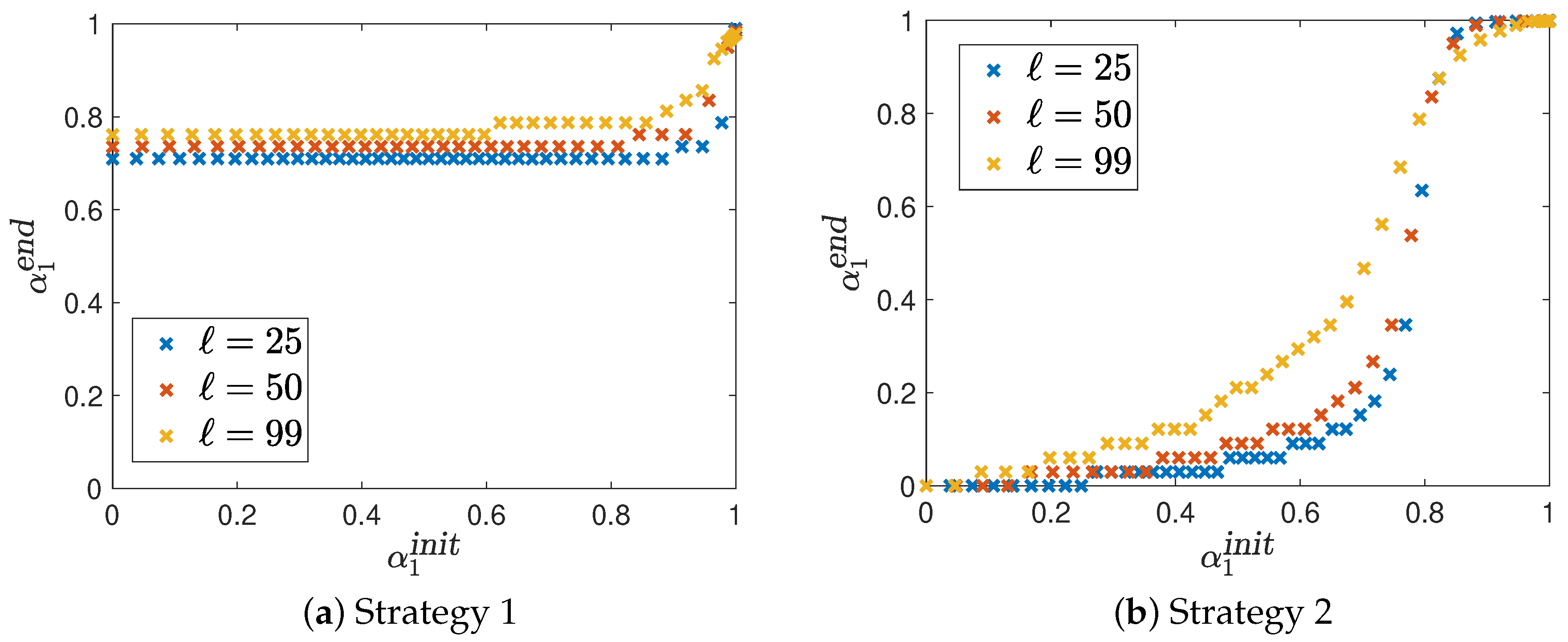
for a weight vector α e n d R 0 2 with α 1 e n d + α 2 e n d = 1 , which can again be determined. The mapping α 1 i n i t α 1 e n d can be seen in Figure 2 for both strategies.
Since the mapping displays the first weight vector, a small value in the plot corresponds to a small weighting of the first cost function (the tracking term) and a large weighting of the second cost function (the control costs), and vice versa.
Note that the ‘ideal’ result of this mapping would be the identity, since this would imply that the weight α i n i t of the initial control u ¯ 0 remains constant throughout the MOMPC algorithm.
From this plot the clustering of the MOMPC points for both strategies can be deduced. For strategy 1 it can be seen that the clustering of the points happen at a weight of α 1 e n d [ 0.7 , 0.8 ] for all MPC horizon lengths. Up to an initial weight of α 1 i n i t 0.8 all the initial controls lead more or less to the same result of the MOMPC algorithm. Only for initial controls with an initial weight of α 1 i n i t > 0.8 , we observe that the upper part of the Pareto front can be reached.
For strategy 2 the clustering in the lower part of the Pareto front for MPC horizon lengths of = 25 and = 50 can be deduced, since up to an initial weight of α 1 i n i t 0.8 , the value of α 1 e n d stays below a value of 0.1, which means that the resulting MOMPC point is in a region of the Pareto front, where the cost function J ^ 2 ( 0 , 1 ) ( · , y ) is weighted much more in comparison to the first cost function J ^ 1 ( 0 , 1 ) ( · , y ) . Moreover, for these two MPC horizons, we can see a clear cut-off behavior at a value of 0.8. If α 1 i n i t is larger than 0.8, the value of α 1 e n d is larger than 0.9. For an MPC horizon length of = 99 , we do not observe such a clear cut-off behavior. Although the plot is still far from being the identity, it is visible that one can control the outcome of the MOMPC algorithm more precisely by varying the initial control.
In conclusion we can say that for strategy 2 a larger MPC horizon leads to a better distribution of the MOMPC points on the Pareto front, and that it is possible to approximate the full scale of the Pareto front by choosing different initial controls u 0 U o p t 0 ( y ) . Strategy 1, however, seems not to be well-suited for this problem framework, since it is not possible to reach to whole extent of the Pareto front by choosing different initial controls. Quite on the contrary, the MOMPC algorithm steers almost all initial controls to the same region of the Pareto front, independently of the MPC horizon length.
Test 2. Now we want to show why the use of MPC in the multiobjective context is needed. For this we consider the following setup: Imagine that we want to compute the Pareto front J o p t ( 0 , 1 ) ( y ) . However, there is only a prediction of the advection field available, which is given by
c p r e d ( t , x ) = ( 1 , 1 ) for all ( t , x ) [ 0 , T ] × Ω .
In the end it turns out that the prediction of the advection field is not very accurate, and the true advection is given by the function c in (14), that is, it deviates from the prediction c p r e d after t = 0.5 .
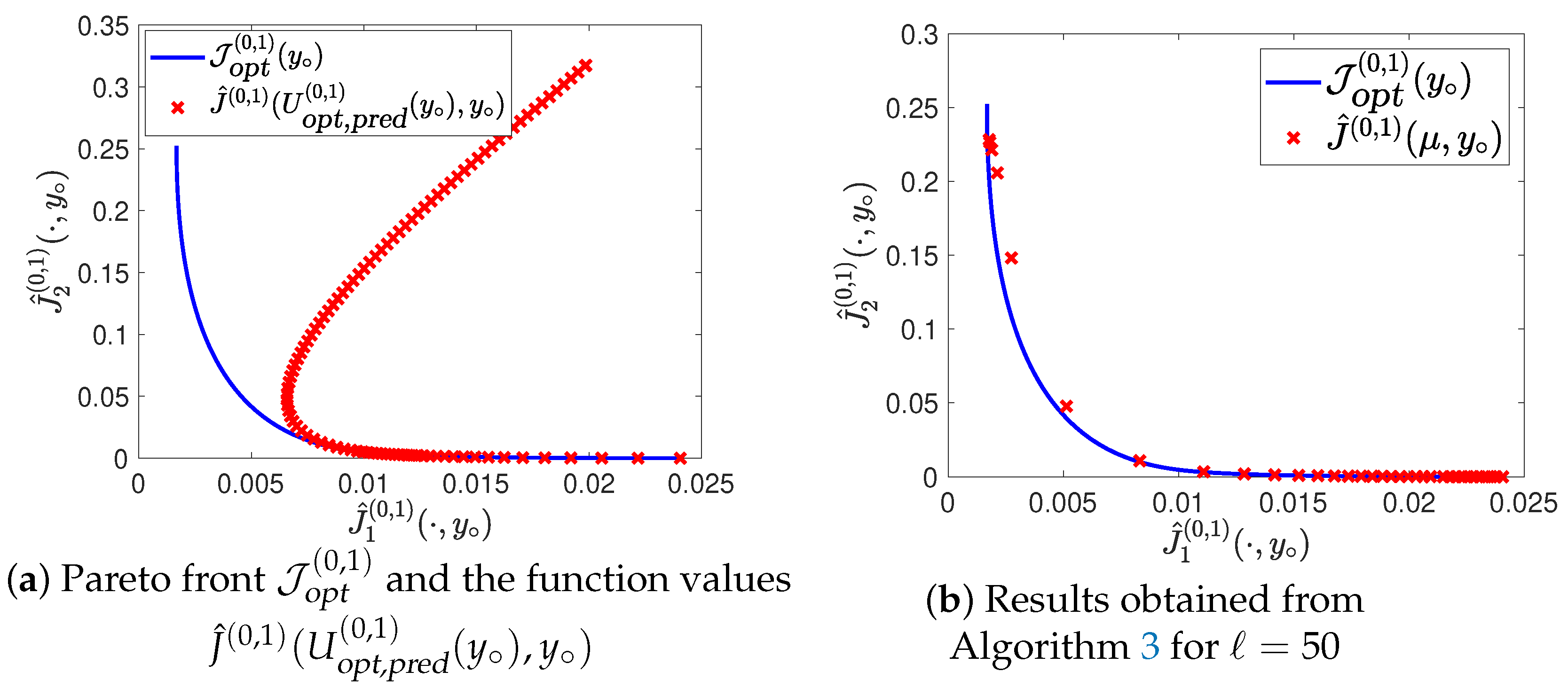
Denote by U o p t , p r e d ( 0 , 1 ) ( y ) the Pareto set of the problem (MOCP) using the predicted advection c p r e d . Again we used the Euclidean reference point method to compute an approximation both of U o p t ( 0 , 1 ) ( y ) and of U o p t , p r e d ( 0 , 1 ) ( y ) . Figure 3a displays the Pareto front J o p t ( 0 , 1 ) ( y ) together with the function values J ^ ( 0 , 1 ) ( U o p t , p r e d ( 0 , 1 ) ( y ) , y ) . One can clearly see that the controls in U o p t , p r e d ( 0 , 1 ) ( y ) are far from being Pareto optimal for the problem with advection c, especially in the upper part of the Pareto front. This can be explained by the fact that the changing advection totally changes the strategy that has to be used to come close to the desired temperature, which is not captured by the open-loop problem using the prediction c p r e d .
We compare this to the results obtained by using the MOMPC Algorithm 3 together with strategy 2 from the first test, where we assumed that the true advection is known to the open-loop problems in the MPC algorithm. This is reasonable since the MPC horizons are reasonably small to allow a precise prediction of the future behavior of the advection field. Just as an example we look at an MPC horizon length of = 50 in Figure 3b and see that in contrast to the predicted Pareto optimal controls U o p t , p r e d ( 0 , 1 ) ( y ) the MOMPC feedback control μ comes quite close to the true Pareto front. This underlines that the use of MOMPC is necessary in situations, in which there are only predictions of data available.

4.2. Example 2

The parameter choices of the previous experiment imply that the choice of a feedback κ fulfilling (7) is not possible. In this section we want to present numerical results for a setup that allows such a feedback in principle.
To this end we choose the following parameter values: The diffusion coefficient is set to d = 0.5 , the reaction coefficient to r = 0.5 , and the advection field is chosen as
c ( t , x ) = ( 1 , 0 ) , if x 2 0.5 , ( 1 , 0 ) , if x 2 0.5 .
As initial condition we choose
y ( x ) = 3 · ( 1 + tanh ( ( x 1 0.5 ) / 0.2 ) ) + 3 ,
which is a smooth approximation of the discontinuous function
x 3 , if x 1 0.5 , 3 , if x 1 0.5 .
It can be shown that y = 0 is a stable steady state of the PDE (1) to the control u = 0 . Therefore, we choose the desired temperatures y 1 1 = y 2 1 = 0 L 2 ( 0 , 1 ; H ) and y 1 2 = y 2 2 = 0 H together with the parameter values σ 1 1 = σ 2 1 = 1 , σ 1 2 = σ 2 2 = 0.1 and σ 1 3 = σ 2 3 = 0.1 . The linear functionals in the cost functions are given by
C 1 1 : L 2 ( 0 , 1 ; H ) L 2 ( 0 , 1 ; H ) , f f · χ { ( t , x ) x 1 0.5 } + 0.01 χ { ( t , x ) x 1 0.5 } , C 2 1 : L 2 ( 0 , 1 ; H ) L 2 ( 0 , 1 ; H ) , f f · 0.01 χ { ( t , x ) x 1 0.5 } + χ { ( t , x ) x 1 0.5 } , C 1 2 : H H , f f · χ { x x 1 0.5 } + 0.01 χ { x x 1 0.5 } , C 2 2 : H H , f f · 0.01 χ { x x 1 0.5 } + χ { x x 1 0.5 } .
Thus, both cost functions measure the deviation of the state from the steady state y = 0 together with some control costs. To make the cost functions conflicting, the linear functionals are chosen such that the first cost function penalizes deviations from the steady state mostly in the left half of the domain, whereas the second cost function penalizes the deviation in the right half of the domain.
If we run Algorithm 3 with this parameter setting, we still observe that in many iterations there is no feedback κ fulfilling (7), especially for the larger MPC horizons of = 25 and = 50 . The reason for this is that the initial Pareto front J o p t 0 ( y ) is quite close or even dominates the Pareto front J o p t ( 0 , 1 ) ( y ) in some points for a MPC horizon of = 25 or = 50 , see Figure 4.
Since the MOMPC points cannot perform better than any point on the Pareto front J o p t ( 0 , 1 ) ( y ) , it is not possible to achieve the performance result from Theorem 3 in those parts. As all the other assumptions of Theorem 3 are satisfied, the reason for not achieving the performance result has to be that it is not possible to find a feedback κ fulfilling (7) in all steps of the algorithm. This is what we observe numerically.
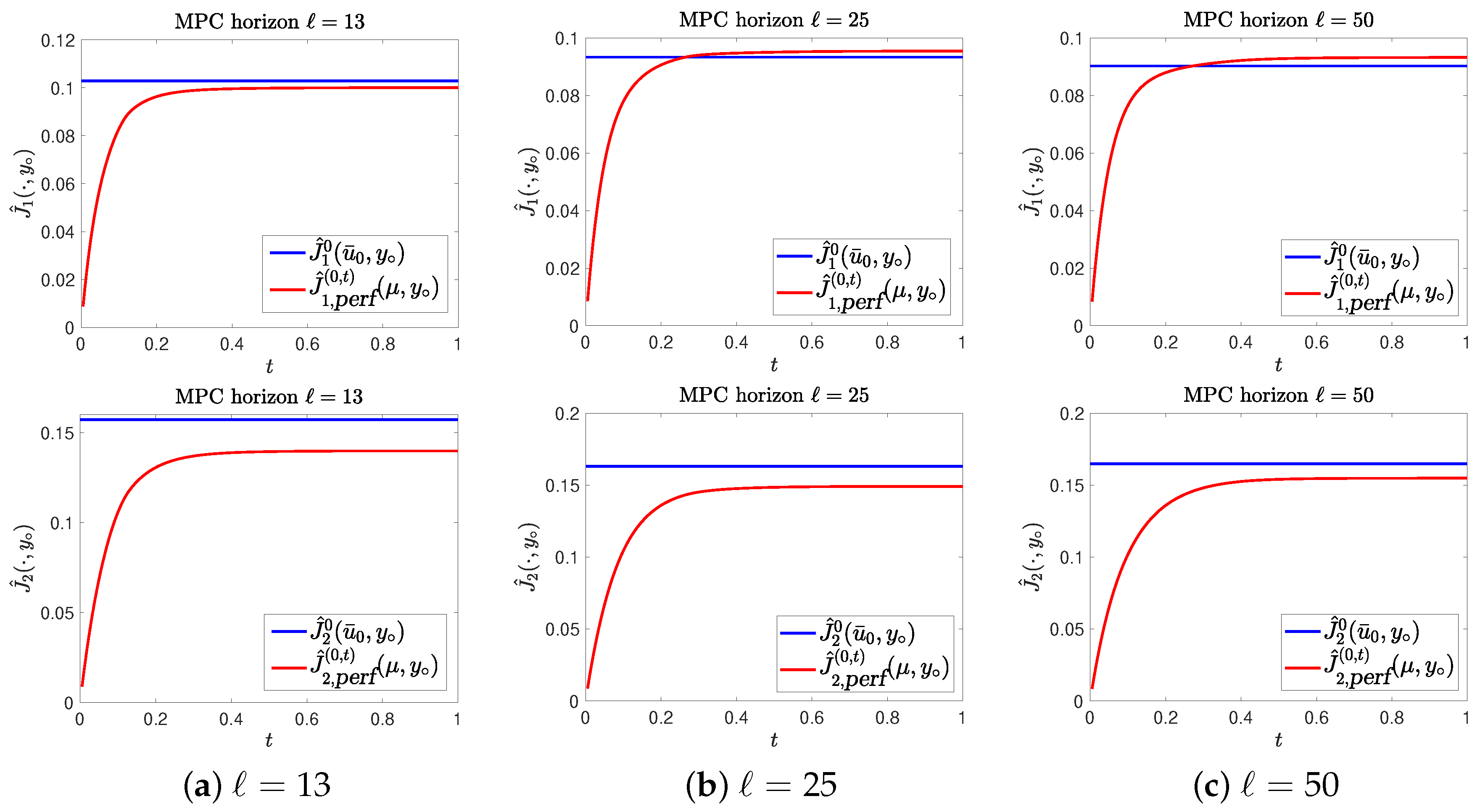
However, if we look at Figure 5 we see that we still obtain the performance result from Theorem 3 for many points, although a feedback κ cannot be found for all these points. The black lines indicate which performance value J ^ corresponds to which initial cost. Therefore, if the black lines are pointing to the top right (starting from the red point), this means that the performance result is satisfied for this point. We observe that the performance result holds for all points for an MPC horizon length of = 13 and for most points for = 25 . Even for = 50 there are some points in the middle of the Pareto front, for which the performance result holds, although there are only very few steps, where a feedback κ fulfilling (7) can be found. Figure 6 indicates that this performance behavior does not change drastically, if we increase the time horizon t end .
The reason for this is that at time t end = 1 the steady state y = 0 is almost reached, so that almost no further costs are needed after this point.
If we compare the MOMPC results obtained from Algorithm 3 with the Pareto front J o p t ( 0 , 1 ) ( y ) of the open-loop problem in Figure 7, we observe that increasing the MPC horizon has two positive effects on the results: Firstly, the MOMPC points are located closer to the Pareto front, and secondly, they are spread more evenly over the entire Pareto front. Already for an MPC horizon length of = 50 we can see that the Pareto front is almost perfectly approximated.

5. Conclusions and Outlook

In this paper we have adopted the framework of MOMPC presented in References [10,11] for ODEs to parabolic advection-diffusion-reaction equations. A key ingredient for the MOMPC algorithm is a gradient-based descent scheme for multiobjective optimization taken from Reference [25,26]. On the one hand, this scheme results in a Pareto optimal point, and on the other hand, it intrinsically implies that the crucial condition (5) is satisfied. Assuming the existence of a feedback κ satisfying (7) we could show that the performance result from ([10], Theorem 11) also holds for our framework of the MOMPC algorithm. Numerically, it turns out that it is hard to guarantee that such a feedback exists. However, even in the case that such a feedback does not exist, the results of the MOMPC algorithm are comparable with the Pareto optimal points of the full-horizon open-loop problem. Especially when some parameters of the PDE can only be predicted, the MOMPC algorithm turns out to be a useful tool, if we still want to compute many compromises between the cost functions.
Both the analysis in Section 3 and the numerical experiments in Section 4 were only carried out for two cost functions, but it is possible to extend both to an arbitrary number of cost function as long as all cost functions are of the form (2). For the analysis this extension is straight-forward, since all the arguments can be transferred directly to this more general case. On the numerical side we can still use the Euclidean reference point method for computing the initial Pareto set U o p t 0 ( y ) , see for example, Reference [29]. In general, the effort for computing the Pareto set U o p t 0 ( y ) scales exponentially with the number of cost functions. However, this computation has only to be performed once in step 4 of Algorithm 3, which is in many cases not underlying any time restrictions. While performing the rest of the MOMPC algorithm the number of cost functions only influences the complexity of steps 6 and 9. In step 6 we need to perform Algorithm 2, in which the dimension of the variable space of the minimization problem (13) is equal to the number of cost functions. Since we only have to compute one Pareto optimal control u ¯ n U o p t n ( y a ) this step is computationally not expensive. In step 9 the number of cost functions in the min-max problem 8 corresponds to the total number of cost functions. Again the effort for solving this problem does not cause complex calculations.
During the MOMPC Algorithm 3 numerous open-loop problems on the MPC horizon have to be solved. Since this involves the solution of the PDE and its associated adjoint equation, this is numerically expensive. Therefore, in a future work one can apply model-order reduction techniques (e.g., the proper orthogonal decomposition method, cf. References [30,31]) for lowering the computational effort. Strategies presented in References [16,17] could be used to show convergence to the full solution.

Author Contributions

All authors have contributes equally. All authors have read and agreed to the published version of the manuscript.

Funding

S.B. and G.F. gratefully acknowledge partially support by the German DFG-Priority Program 1962 and German Science Fund DFG grant “Reduced-Order Methods for Nonlinear Model Predictive Control”, respectively. Moreover, S.B. is partially funded by the German Landesgraduiertenförderung of Baden-Württemberg.

Conflicts of Interest

The authors declare no conflict of interest.

Abbreviations

The following abbreviations are used in this manuscript:
MOMultiobjective optimization
MOPMultiobjective optimization problem
MOCPMultiobjective optimal control problem
MPCModel predictive control
MOMPCMultiobjective model predictive control
ODEOrdinary differential equation
PDEPartial differential equation

References

  1. Rawlings, J.; Mayne, D. Model Predictive Control: Theory and Design; Nob Hill Publishing: Madison, WI, USA, 2009. [Google Scholar]
  2. Forbes, M.G.; Patwardhan, R.S.; Hamadah, H.; Gopaluni, R.B. Model Predictive Control in Industry: Challenges and Opportunities. In Proceedings of the 9th IFAC Symposium on Advanced Control of Chemical Processes—ADCHEM 2015, Whistler, BC, Canada, 7–10 June 2015; Volume 48, pp. 531–538. [Google Scholar]
  3. Grüne, L. Approximation properties of receding horizon optimal control. Jahresbericht der Deutschen Mathematiker-Vereinigung 2016, 118, 3–37. [Google Scholar] [CrossRef] [Green Version]
  4. Grüne, L.; Pannek, J. Nonlinear Model Predictive Control: Theory and Algorithms, 2nd ed.; Communications and Control Engineering; Springer: Berlin/Heidelberg, Germany, 2017. [Google Scholar]
  5. Laabidi, K.; Bouani, F.; Ksouri, M. Multi-criteria optimization in nonlinear predictive control. Math. Comput. Simul. 2008, 76, 363–374. [Google Scholar] [CrossRef]
  6. Bemporad, A.; Muñoz de la Peña, D. Multiobjective model predictive control. Automatica 2009, 45, 2823–2830. [Google Scholar] [CrossRef]
  7. He, D.; Wang, L.; Sun, J. On stability of multiobjective NMPC with objective prioritization. Automatica 2015, 57, 189–198. [Google Scholar] [CrossRef]
  8. Zavala, V.M.; Flores-Tlacuahuac, A. Stability of multiobjective predictive control: A utopia-tracking approach. Automatica 2012, 48, 2627–2632. [Google Scholar] [CrossRef]
  9. Peitz, S.; Schäfer, K.; Ober-Blöbaum, S.; Eckstein, J.; Köhler, U.; Dellnitz, M. A Multiobjective MPC Approach for Autonomously Driven Electric Vehicles. IFAC PapersOnLine 2017, 50, 8674–8679. [Google Scholar] [CrossRef]
  10. Grüne, L.; Stieler, M. Performance guarantees for multiobjective model predictive control. In Proceedings of theIEEE 56th Annual Conference on Decision and Control (CDC), Melbourne, Australia, 12–15 December 2017; pp. 5545–5550. [Google Scholar]
  11. Grüne, L.; Stieler, M. Multiobjective model predictive control for stabilizing cost criteria. Discret. Contin. Dyn. Syst. B 2019, 24, 3905. [Google Scholar] [CrossRef] [Green Version]
  12. Ehrgott, M. Multicriteria Optimization, 2nd ed.; Springer: Berlin/Heidelberg, Germany; New York, NY, USA, 2005. [Google Scholar]
  13. Miettinen, K. Nonlinear Multiobjective Optimization; Springer: New York, NY, USA, 1998. [Google Scholar]
  14. Iapichino, L.; Trenz, S.; Volkwein, S. Multiobjective optimal control of semilinear parabolic problems using POD. In Numerical Mathematics and Advanced Applications (ENUMATH 2015); Karasözen, B., Manguoglu, M., Tezer-Sezgin, M., Goktepe, S., Ugur, Ö., Eds.; Springer: Berlin/Heidelberg, Germany, 2016; pp. 389–397. [Google Scholar]
  15. Iapichino, L.; Ulbrich, S.; Volkwein, S. Multiobjective PDE-constrained optimization using the reduced-basis method. Adv. Comput. Math. 2017, 43, 945–972. [Google Scholar] [CrossRef]
  16. Peitz, S. Exploiting Structure in Multiobjective Optimization and Optimal Control. Ph.D. Thesis, Paderborn University, Paderborn, Germany, 2017. [Google Scholar]
  17. Peitz, S.; Dellnitz, M. Gradient-Based Multiobjective Optimization with Uncertainties. In Proceedings of the NEO 2016: Results of the Numerical and Evolutionary Optimization Workshop NEO 2016 and the NEO Cities 2016 Workshop, Tlalnepantla, Mexico, 20–24 September 2016; Maldonado, Y., Trujillo, L., Schütze, O., Riccardi, A., Vasile, M., Eds.; Springer International Publishing: Cham, Switzerland, 2017; pp. 159–182. [Google Scholar] [CrossRef] [Green Version]
  18. Banhozer, S.; Dellnitz, M.; Gebken, B.; Peitz, S.; Volkwein, S. ROM-based multiobjective optimization of elliptic PDEs via numerical continuation. arXiv 2019, arXiv:1906.09075v1. [Google Scholar]
  19. Wierzbicki, A.P. The Use of Reference Objectives in Multiobjective Optimization. In Multiple Criteria Decision Making Theory and Application; Springer: Berlin/Heidelberg, Germany, 1980; pp. 468–486. [Google Scholar]
  20. Wierzbicki, A.P. On the completeness and constructiveness of parametric characterizations to vector optimization problems. Oper. Res. Spektrum 1986, 8, 73–87. [Google Scholar] [CrossRef]
  21. Banholzer, S.; Beermann, D.; Volkwein, S. POD-Based Bicriterial Optimal Control by the Reference Point Method. IFAC PapersOnLine 2016, 49, 210–215. [Google Scholar] [CrossRef]
  22. Banholzer, S. POD-Based Bicriterial Optimal Control of Convection-Diffusion Equations. Master’s Thesis, University of Konstanz, Konstanz, Germany, 2017. [Google Scholar]
  23. Banholzer, S.; Beermann, D.; Volkwein, S. POD-Based error control for reduced-order bicriterial PDE-constrained optimization. Annu. Rev. Control 2017, 44, 226–237. [Google Scholar] [CrossRef] [Green Version]
  24. Dautray, R.; Lions, J.L. Mathematical Analysis and Numerical Methods for Science and Technology; Volume 5: Evolution Problems I; Springer Science & Business Media: Cham, Switzerland, 2000. [Google Scholar]
  25. Schäffler, S.; Schultz, R.; Weinzierl, K. Stochastic Method for the Solution of Unconstrained Vector Optimization Problems. J. Optim. Theory Appl. 2002, 114, 209–222. [Google Scholar] [CrossRef]
  26. Fliege, J.; Svaiter, B. Steepest descent methods for multicriteria optimization. Math. Methods Oper. Res. 2000, 51, 479–494. [Google Scholar] [CrossRef]
  27. Grüne, L.; Schaller, M.; Schiela, A. Sensitivity analysis of optimal control for a class of parabolic PDEs motivated by model predictive control. SIAM J. Control Optim. 2019, 57, 2753–2774. [Google Scholar] [CrossRef] [Green Version]
  28. Grüne, L.; Schaller, M.; Schiela, A. Exponential sensitivity analysis for Model Predictive Control of PDEs. Preprint, Department of Mathematics, University of Bayreuth. 2020. Available online: http://nbn-resolving.org/urn:nbn:de:bvb:703-epub-4590-3 (accessed on 4 May 2020).
  29. Banholzer, S.; Volkwein, S. Hierarchical Convex Multiobjective Optimization by the Euclidean Reference Point Method; Technical Report; University of Konstanz: Konstanz, Germany, 2019. [Google Scholar]
  30. Sirovich, L. Turbulence and the dynamics of coherent structures part I: Coherent structures. Q. Appl. Math. 1987, 45, 561–571. [Google Scholar] [CrossRef] [Green Version]
  31. Gubisch, M.; Volkwein, S. Proper Orthogonal Decomposition for Linear-Quadratic Optimal Control. In Model Reduction and Approximation: Theory and Algorithms; Benner, P., Cohen, A., Ohlberger, M., Willcox, K., Eds.; SIAM: Philadelphia, PA, USA, 2017; pp. 5–66. [Google Scholar] [CrossRef] [Green Version]
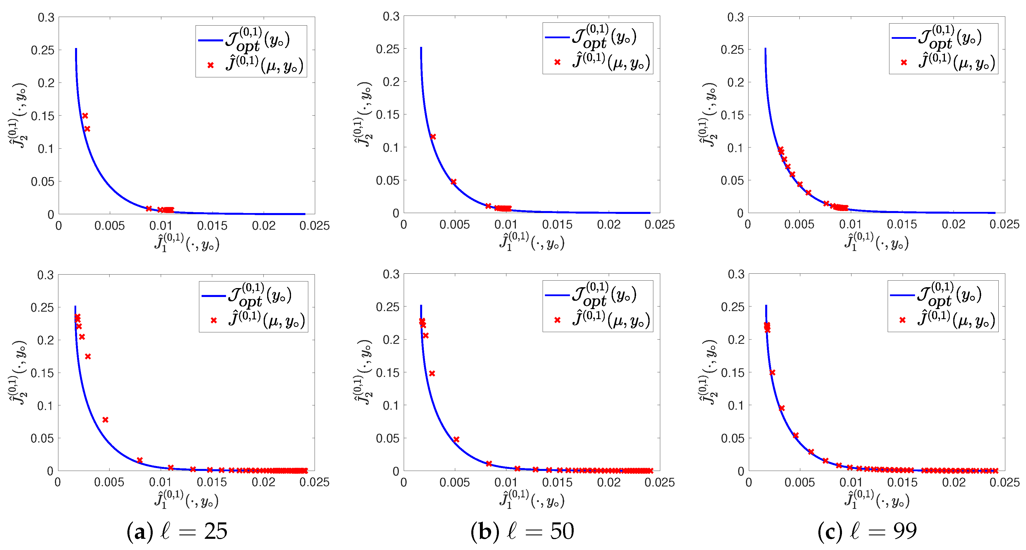
Figure 1. Results of Algorithm 3 for all initial controls u ¯ 0 U o p t , a p p r 0 ( y ) for different horizon lengths. Top: Strategy 1 for computing κ . Bottom: Strategy 2 for computing κ .
Mathematics 08 00777 g001
Figure 2. The mapping α 1 i n i t α 1 e n d for different model predictive control (MPC) horizon lengths.
Mathematics 08 00777 g002
Figure 3. Comparison of the predictive multiobjective optimal control and Algorithm 3.
Mathematics 08 00777 g003
Figure 4. Comparison between J o p t ( 0 , 1 ) ( y ) and J o p t 0 ( y ) for different MPC horizon lengths.
Mathematics 08 00777 g004
Figure 5. Performance Results.
Mathematics 08 00777 g005
Figure 6. Performance Results for the top left point of the Pareto front.
Mathematics 08 00777 g006
Figure 7. Comparison the results from Algorithm 3 and the Pareto front.
Mathematics 08 00777 g007