An Efficient Hybrid Genetic Approach for Solving the Two-Stage Supply Chain Network Design Problem with Fixed Costs


Abstract
:1. Introduction
- The two-stage transportation problem with fixed costs associated with the routes: Raj and Rajendran [12] proposed two scenarios of the two-stage transportation problem: the first one, called Scenario 1, takes into consideration fixed costs associated with the routes in addition to unit transportation costs and boundless capacities of the DCs, while the second one, called Scenario 2, considers the opening costs of the DCs in addition to unit transportation costs. The same authors developed a genetic algorithm (GA) with a particular coding scheme applicable for two-stage transportation problems, and also, they provided a set of 20 benchmark instances. Another GA dealing with the two-stage transportation problem with fixed charge associated with the routes from plants to customers through DCs was proposed by Jawahar and Balaji [13]. Pop et al. [14] proposed a hybrid method that combines a steady-state GA with a powerful local search procedure. Cosma et al. [15] described an efficient multi-start iterated local search (ILS) procedure for the total transportation cost minimization of the two-stage transportation problem, which begins with a feasible solution of the problem, makes use of a local search procedure with the goal of increasing the exploration, a perturbation mechanism, and a neighborhood operator with the scope of diversifying the search.
- The two-stage transportation problem with fixed costs for opening the distribution centers (DCs): This two-stage transportation problem was introduced by Gen et al. [16]. The present literature regarding the two-stage transportation problem with fixed costs for opening the DCs is rather limited. This optimization problem has also been investigated by Raj and Rajendran [12], who called it Scenario 2. Calvete et al. [17] proposed a hybrid evolutionary algorithm whose principal characteristic is the employment of a chromosome encoding that offers information about the DCs used within the transportation system. Cosma et al. [18] described an effective heuristic algorithm that reduces the solution search space to a subspace with a reasonable size, without losing optimal or sub-optimal solutions by means of a perturbation mechanism that allows the reconsideration of the feasible solutions that are discarded and that might lead to such solutions. Lately, Cosma et al. [19] proposed a matheuristic approach for solving the two-stage transportation problem with fixed costs associated with the routes by incorporating a linear programming optimization problem within the framework of a genetic algorithm.
- A particular case is where there exists only one plant manufacturer, and this version was considered by Molla et al. [20]. They proposed an integer linear programming mathematical model of the problem, and in addition, they described two solution approaches for solving it: a spanning tree-based genetic algorithm with a Prüfer number representation and an artificial immune algorithm. Some remarks regarding the mathematical model of the problem were published by El-Sherbiny [21]. Pintea et al. [22] proposed some hybrid algorithms, and Pintea and Pop [23] described an efficient hybrid approach combining the nearest neighbor search heuristic with a local search procedure for solving this particular two-stage transportation problem with fixed costs. Pop et al. [24] developed an innovative hybrid heuristic method achieved by combining a genetic algorithm based on a hash table coding of the individuals with a powerful local search procedure. Recently, Cosma et al. [25] described an effective hybrid heuristic approach that builds an initial feasible solution, then uses a local search procedure whose goal is to increase the exploration and a neighborhood structure for diversifying the search.
- Another two-stage transportation problem takes into consideration its effect on the environment by reducing the greenhouse gas emissions and was introduced by Santibanez-Gonzales [26] for dealing with a practical application from the public sector. For this version of the problem, Pintea et al. [27] described a set of hybrid heuristic methods, and Pop et al. [28] proposed an effective reverse distribution system for solving it.
2. Definition of the Two-Stage Supply Chain Network Design Problem with Fixed Costs for Opening the Distribution Centers and Transportation Routes
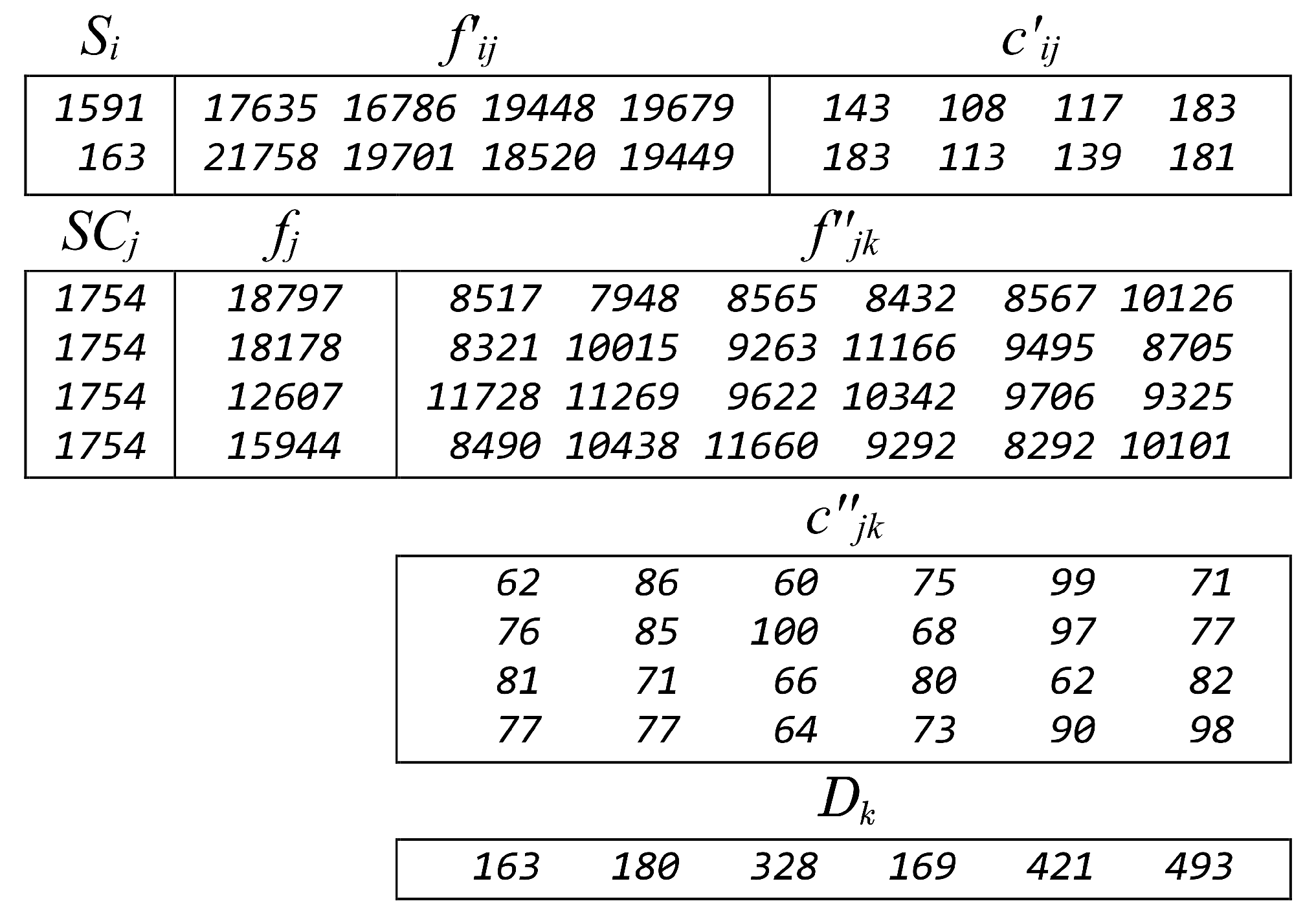
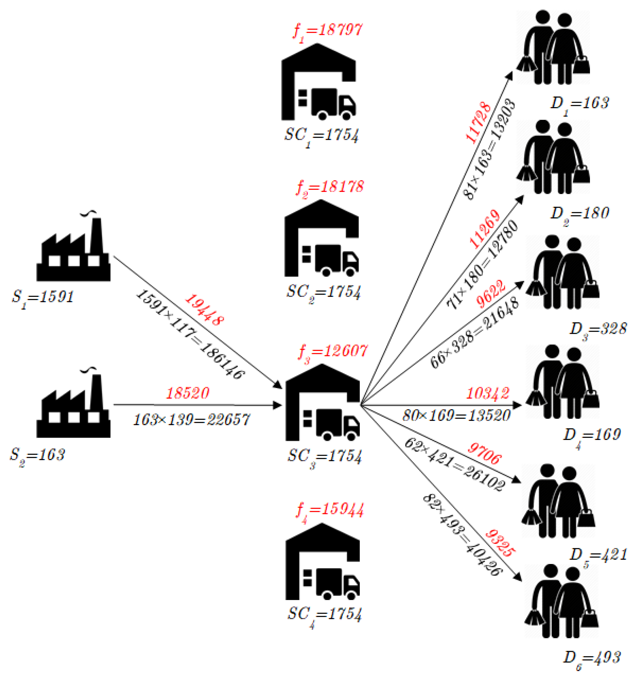
- Every manufacturer has units of supply; every distribution center has a given capacity ; each customer has a demand ;
- Every manufacturer may transport to any of the q distribution centers at a transportation cost per unit from manufacturer to DC ;
- Every DC may transport to any of the r customers at a transportation cost per unit from DC to customer ;
- In order to open any of the DCs, we have to pay a given fixed cost denoted by , and there exist fixed transportation costs from each manufacturer to each distribution center, denoted by , where and , and from each DC to each customer, denoted by , where and .
3. A Valid Mathematical Model of the Two-Stage Supply Chain Network Design Problem with Fixed Costs
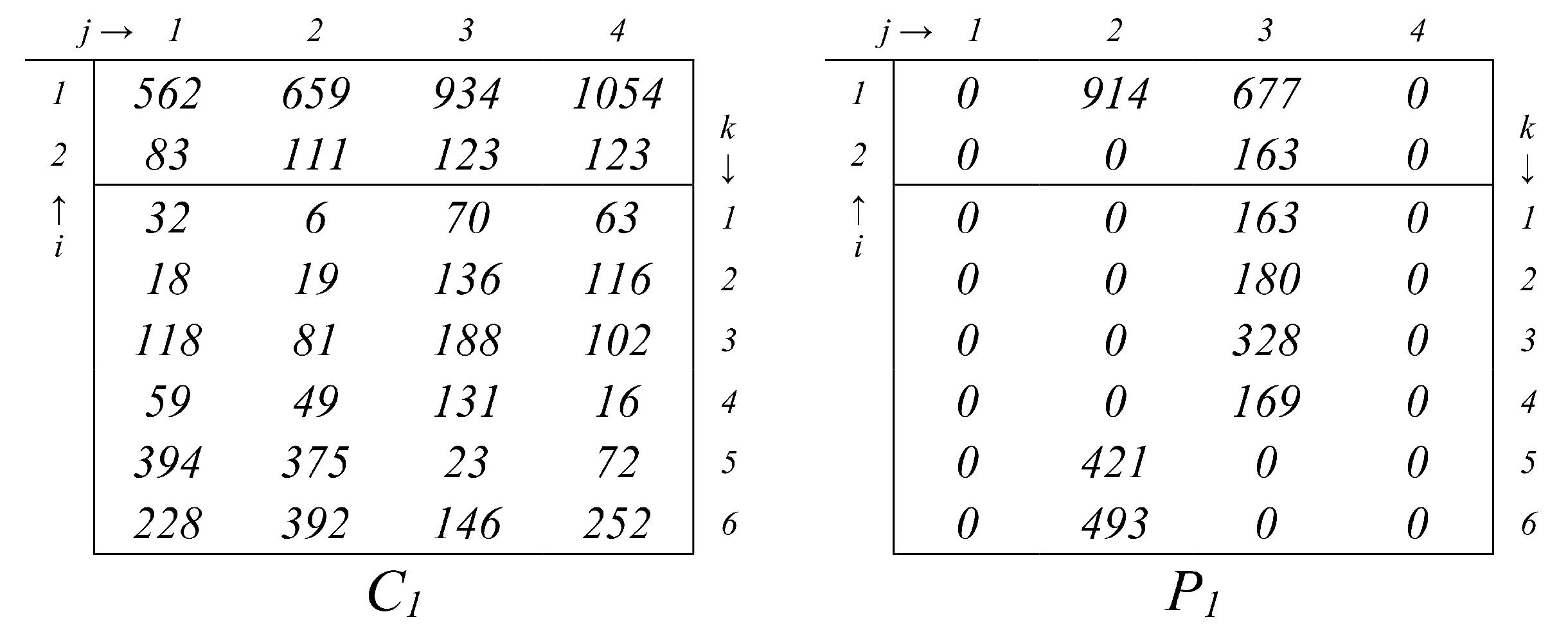
- Linear variables:
- -
- , specifying the number of units shipped from plant i to the DC j;
- -
- , specifying the number of units shipped from DC j to the customer k;
- Binary variables:
- -
- , specifying if there are units transported from manufacturer plant i to the DC j (, if , and , otherwise);
- -
- , specifying if there are units transported from DC j to the customer k (, if , and , otherwise);
- -
- , specifying if the DC j is open (, if the DC j is open, and , otherwise).
4. Description of the Novel Solution Approach
| Algorithm 1: Procedure Chromosome enhancement |
 |
- The first two-thirds of the current population will be completed with the best chromosomes in the pool. At least half of these chromosomes must be newborn, i.e., not being part of the current population in the previous stages of evolution.
- The other chromosomes in the current population are randomly chosen from the pool.
5. Discussion
- In the case of small and medium sized instances, our algorithm delivered the optimal solution in all ten runs of each instance, but with much less computational time effort in comparison to CPLEX.
- As regards the 50 large sized instances, for seven of them, our hybrid algorithm delivered the optimal solution in all ten runs of each instance, but with much less computational time effort in comparison to CPLEX, and for the remaining instances, the best solution achieved by our algorithm improved the solution provided by CPLEX within 3600 s, but with much less computational time effort in comparison to CPLEX.
- In the case of the proposed 50 larger instances, the best solution provided by our hybrid genetic algorithm improved the solution delivered by CPLEX within 3600 s, and the average computational times spent in solving the corresponding instances were lower compared to CPLEX.
- We can remark that our developed solution outperformed in terms of the quality of the solutions and of computational times the ACO-based heuristic approach proposed by Hong et al. [10], which according to the previously mentioned authors, provided sub-optimal solutions with a gap of about on average from the optimal solutions.
6. Conclusions
Author Contributions
Funding
Acknowledgments
Conflicts of Interest
References
- Govindan, K.; Fattahi, M.; Keyvanshokooh, E. Supply chain network design under uncertainty: A comprehensive review and future research directions. Eur. J. Oper. Res. 2017, 263, 108–141. [Google Scholar] [CrossRef]
- Klibi, W.; Martel, A.; Guitouni, A. The design of robust value-creating supply chain networks: A critical review. Eur. J. Oper. Res. 2010, 203, 283–293. [Google Scholar] [CrossRef]
- Melo, M.T.; Nickel, S.; Da Gamma, F.S. Facility location and supply chain management—A review. Eur. J. Oper. Res. 2009, 196, 401–412. [Google Scholar] [CrossRef]
- Wang, H.S. A two-phase ant colony algorithm for multi-echelon defective supply chain netwok design. Eur. J. Oper. Res. 2009, 192, 243–252. [Google Scholar] [CrossRef]
- Dotoli, M.; Fanti, M.P.; Meloni, C.; Zhou, M.C. A Multi-Level Approach for Network Design of Integrated Supply Chains. Int. J. Prod. Res. 2005, 43, 4267–4287. [Google Scholar] [CrossRef]
- Dotoli, M.; Fanti, M.P.; Meloni, C.; Zhou, M.C. A decision support system for the supply chain configuration. IEEE Int. Conf. Syst. Man Cybern. 2003, 3, 2667–2672. [Google Scholar]
- Balinski, M.I. Fixed-cost transportation problems. Nav. Res. Logist. 1961, 8, 41–54. [Google Scholar] [CrossRef]
- Guisewite, G.; Pardalos, P. Minimum concave-cost network flow problems: Applications, complexity, and algorithms. Ann. Oper. Res. 1990, 25, 75–99. [Google Scholar] [CrossRef]
- Buson, E.; Roberti, R.; Toth, P. A reduced-cost iterated local search heuristic for the fixed-charge transportation problem. Oper. Res. 2014, 62, 1095–1106. [Google Scholar] [CrossRef] [Green Version]
- Hong, J.; Diabat, A.; Panicker, V.V.; Rajagopalan, S. A two-stage supply chain problem with fixed costs: An ant colony optimization approach. Int. J. Prod. Econ. 2018, 204, 214–226. [Google Scholar] [CrossRef]
- Sabo, C.; Horvat-Marc, A.; Pop, P.C. Comments on “A two-stage supply chain problem with fixed costs: An ant colony optimization approach” by Hong et al. International Journal of Production Economics (2018). Creat. Math. Inform. 2019, 28, 183–189. [Google Scholar]
- Raj, K.A.A.D.; Rajendran, C. A genetic algorithm for solving the fixed-charge transportation model: Two-stage problem. Comput. Oper. Res. 2012, 39, 2016–2032. [Google Scholar]
- Jawahar, N.; Balaji, A.N. A genetic algorithm for the two-stage supply chain distribution problem associated with a fixed charge. Eur. J. Oper. Res. 2009, 194, 496–537. [Google Scholar] [CrossRef]
- Pop, P.C.; Sabo, C.; Biesinger, B.; Hu, B.; Raidl, G. Solving the Two-Stage Fixed-Charge Transportation Problem with a Hybrid Genetic Algorithm. Carpathian J. Math. 2017, 33, 365–371. [Google Scholar]
- Cosma, O.; Pop, P.C.; Pop Sitar, C. An efficient iterated local search heuristic algorithm for the two-stage fixed-charge transportation problem. Carpathian J. Math. 2019, 35, 153–164. [Google Scholar]
- Gen, M.; Altiparmak, F.; Lin, L. A genetic algorithm for two-stage transportation problem using priority based encoding. OR Spectr. 2006, 28, 337–354. [Google Scholar] [CrossRef]
- Calvete, H.; Gale, C.; Iranzo, J. An improved evolutionary algorithm for the two-stage transportation problem with fixed charge at depots. OR Spectr. 2016, 38, 189–206. [Google Scholar] [CrossRef]
- Cosma, O.; Dănciulescu, D.; Pop, P.C. On the two-stage transportation problem with fixed charge for opening the distribution centers. IEEE Access 2019, 79, 113684–113698. [Google Scholar] [CrossRef]
- Cosma, O.; Pop, P.C.; Dănciulescu, D. A novel matheuristic approach for a two-stage transportation problem with fixed costs associated with the routes. Comput. Oper. Res. 2020, 118, 104906. [Google Scholar] [CrossRef]
- Molla-Alizadeh-Zavardehi, S.; Hajiaghaei-Kesteli, M.; Tavakkoli-Moghaddam, R. Solving a capacitated fixed-cost transportation problem by artificial immune and genetic algorithms with a Prüfer number representation. Expert Syst. Appl. 2011, 38, 10462–10474. [Google Scholar] [CrossRef]
- El-Sherbiny, M.M. Comments on “Solving a capacitated fixed-cost transportation problem by artificial immune and genetic algorithms with a Prüfer number representation" by Molla-Alizadeh-Zavardehi, S. et al. Expert Syst. Appl. Expert Syst. Appl. 2012, 39, 11321–11322. [Google Scholar] [CrossRef]
- Pintea, C.-M.; Pop Sitar, C.; Hajdu-Macelaru, M.; Pop, P.C. A Hybrid Classical Approach to a Fixed-Charge Transportation Problem. In Proceedings of HAIS 2012, Part I Lecture Notes in Computer Science; Corchado, E., Ed.; Springer: Salamanca, Spain, 2012; Volume 7208, pp. 557–566. [Google Scholar]
- Pintea, C.M.; Pop, P.C. An improved hybrid algorithm for capacitated fixed-charge transportation problem. Log. J. IJPL 2015, 23, 369–378. [Google Scholar] [CrossRef]
- Pop, P.C.; Matei, O.; Pop Sitar, C.; Zelina, I. A hybrid based genetic algorithm for solving a capacitated fixed-charge transportation problem. Carpathian J. Math. 2016, 32, 225–232. [Google Scholar]
- Cosma, O.; Pop, P.C.; Matei, O.; Zelina, I. A hybrid iterated local search for solving a particular two-stage fixed-charge transportation problem. In Proceedings of HAIS 2018, Lecture Notes in Computer Science; Springer: Oviedo, Spain, 2018; Volume 10870, pp. 684–693. [Google Scholar]
- Santibanez-Gonzalez, E.D.R.; Robson Mateus, G.; Pacca Luna, H. Solving a public sector sustainable supply chain problem: A Genetic Algorithm approach. In Proceedings of the International Conference on Artificial Intelligence (ICAI), Las Vegas, NV, USA, 18–21 July 2011; pp. 507–512. [Google Scholar]
- Pintea, C.-M.; Pop, P.C.; Hajdu-Măcelaru, M. Classical Hybrid Approaches on a Transportation Problem with Gas Emissions Constraints. Adv. Intell. Soft Comput. 2013, 188, 449–458. [Google Scholar]
- Pop, P.C.; Pintea, C.-M.; Pop Sitar, C.; Hajdu-Macelaru, M. An efficient Reverse Distribution System for solving sustainable supply chain network design problem. J. Appl. Log. 2015, 13, 105–113. [Google Scholar] [CrossRef]
- Holland, J.H. Adaptation in Natural and Artificial Systems: An Introductory Analysis with Applications to Biology. In Control and Artificial Intelligence; MIT Press: Cambridge, MA, USA, 1992. [Google Scholar]
- Two Stage Transportation Problem Instances. Available online: https://sites.google.com/view/tstp-instances/ (accessed on 26 April 2020).


| Instance | CPLEX | Our Proposed Hybrid Genetic Algorithm | Improvement | ||||||
|---|---|---|---|---|---|---|---|---|---|
| % | Time (%) | ||||||||
| 1. | 150,787 | 0.047 | 150,787 | 150,787 | 0.00 | 0.000 | 0.000 | 0.000 | 100.0 |
| 2. | 156,654 | 0.047 | 156,654 | 156,654 | 0.00 | 0.000 | 0.000 | 0.000 | 100.0 |
| 3. | 139,811 | 0.047 | 139,811 | 139,811 | 0.00 | 0.000 | 0.000 | 0.000 | 100.0 |
| 4. | 128,859 | 0.047 | 128,859 | 128,859 | 0.00 | 0.000 | 0.000 | 0.000 | 100.0 |
| 5. | 116,637 | 0.093 | 116,637 | 116,637 | 0.00 | 0.000 | 0.015 | 0.002 | 98.4 |
| 6. | 87,694 | 0.078 | 87,694 | 87,694 | 0.00 | 0.000 | 0.016 | 0.002 | 97.9 |
| 7. | 105,420 | 0.063 | 105,420 | 105,420 | 0.00 | 0.000 | 0.015 | 0.002 | 97.6 |
| 8. | 120,077 | 0.063 | 120,077 | 120,077 | 0.00 | 0.000 | 0.015 | 0.002 | 97.6 |
| 9. | 117,590 | 0.063 | 117,590 | 117,590 | 0.00 | 0.000 | 0.016 | 0.002 | 97.5 |
| 10. | 131,233 | 0.063 | 131,233 | 131,233 | 0.00 | 0.000 | 0.016 | 0.002 | 97.5 |
| 11. | 121,411 | 0.062 | 121,411 | 121,411 | 0.00 | 0.000 | 0.016 | 0.002 | 97.4 |
| 12. | 149,525 | 0.109 | 149,525 | 149,525 | 0.00 | 0.000 | 0.016 | 0.003 | 97.1 |
| 13. | 134,591 | 0.156 | 134,591 | 134,591 | 0.00 | 0.000 | 0.016 | 0.005 | 97.0 |
| 14. | 105,047 | 0.047 | 105,047 | 105,047 | 0.00 | 0.000 | 0.015 | 0.002 | 96.8 |
| 15. | 127,184 | 0.047 | 127,184 | 127,184 | 0.00 | 0.000 | 0.015 | 0.002 | 96.8 |
| 16. | 122,630 | 0.094 | 122,630 | 122,630 | 0.00 | 0.000 | 0.016 | 0.003 | 96.7 |
| 17. | 101,722 | 0.094 | 101,722 | 101,722 | 0.00 | 0.000 | 0.016 | 0.003 | 96.7 |
| 18. | 132,593 | 0.047 | 132,593 | 132,593 | 0.00 | 0.000 | 0.016 | 0.002 | 96.6 |
| 19. | 113,976 | 0.047 | 113,976 | 113,976 | 0.00 | 0.000 | 0.016 | 0.002 | 96.6 |
| 20. | 129,436 | 0.172 | 129,436 | 129,436 | 0.00 | 0.000 | 0.016 | 0.006 | 96.4 |
| 21. | 146,078 | 0.125 | 146,078 | 146,078 | 0.00 | 0.000 | 0.016 | 0.005 | 96.2 |
| 22. | 119,627 | 0.079 | 119,627 | 119,627 | 0.00 | 0.000 | 0.016 | 0.003 | 96.1 |
| 23. | 95,845 | 0.078 | 95,845 | 95,845 | 0.00 | 0.000 | 0.016 | 0.003 | 96.0 |
| 24. | 104,190 | 0.078 | 104,190 | 104,190 | 0.00 | 0.000 | 0.016 | 0.003 | 95.9 |
| 25. | 127,869 | 0.140 | 127,869 | 127,869 | 0.00 | 0.000 | 0.016 | 0.006 | 95.6 |
| 26. | 100,451 | 0.171 | 100,451 | 100,451 | 0.00 | 0.000 | 0.016 | 0.008 | 95.4 |
| 27. | 128,253 | 0.094 | 128,253 | 128,253 | 0.00 | 0.000 | 0.016 | 0.005 | 95.1 |
| 28. | 150,379 | 0.125 | 150,379 | 150,379 | 0.00 | 0.000 | 0.016 | 0.006 | 95.0 |
| 29. | 108,942 | 0.093 | 108,942 | 108,942 | 0.00 | 0.000 | 0.016 | 0.005 | 94.9 |
| 30. | 137,955 | 0.062 | 137,955 | 137,955 | 0.00 | 0.000 | 0.016 | 0.003 | 94.8 |
| 31. | 170,119 | 0.109 | 170,119 | 170,119 | 0.00 | 0.000 | 0.016 | 0.006 | 94.3 |
| 32. | 126,603 | 0.079 | 126,603 | 126,603 | 0.00 | 0.000 | 0.016 | 0.005 | 94.2 |
| 33. | 134,653 | 0.078 | 134,653 | 134,653 | 0.00 | 0.000 | 0.016 | 0.005 | 94.1 |
| 34. | 142,559 | 0.078 | 142,559 | 142,559 | 0.00 | 0.000 | 0.016 | 0.005 | 94.0 |
| 35. | 126,611 | 0.125 | 126,611 | 126,611 | 0.00 | 0.000 | 0.032 | 0.008 | 93.8 |
| 36. | 116,869 | 0.047 | 116,869 | 116,869 | 0.00 | 0.000 | 0.015 | 0.003 | 93.6 |
| 37. | 108,201 | 0.094 | 108,201 | 108,201 | 0.00 | 0.000 | 0.016 | 0.006 | 93.4 |
| 38. | 129,005 | 0.047 | 129,005 | 129,005 | 0.00 | 0.000 | 0.016 | 0.003 | 93.2 |
| 39. | 127,997 | 0.110 | 127,997 | 127,997 | 0.00 | 0.000 | 0.016 | 0.008 | 92.9 |
| 40. | 104,891 | 0.109 | 104,891 | 104,891 | 0.00 | 0.000 | 0.047 | 0.008 | 92.8 |
| 41. | 111,104 | 0.063 | 111,104 | 111,104 | 0.00 | 0.000 | 0.016 | 0.005 | 92.7 |
| 42. | 108,001 | 0.062 | 108,001 | 108,001 | 0.00 | 0.000 | 0.016 | 0.005 | 92.6 |
| 43. | 143,700 | 0.063 | 143,700 | 143,700 | 0.00 | 0.000 | 0.016 | 0.005 | 92.5 |
| 44. | 138,510 | 0.078 | 138,510 | 138,510 | 0.00 | 0.000 | 0.016 | 0.006 | 92.1 |
| 45. | 135,101 | 0.079 | 135,101 | 135,101 | 0.00 | 0.000 | 0.016 | 0.006 | 92.0 |
| 46. | 129,854 | 0.078 | 129,854 | 129,854 | 0.00 | 0.000 | 0.016 | 0.006 | 91.9 |
| 47. | 116,670 | 0.094 | 116,670 | 116,670 | 0.00 | 0.000 | 0.016 | 0.008 | 91.8 |
| 48. | 141,467 | 0.047 | 141,467 | 141,467 | 0.00 | 0.000 | 0.016 | 0.005 | 90.2 |
| 49. | 141,306 | 0.094 | 141,306 | 141,306 | 0.00 | 0.000 | 0.031 | 0.009 | 90.1 |
| 50. | 125,550 | 0.062 | 125,550 | 125,550 | 0.00 | 0.000 | 0.016 | 0.006 | 90.0 |
| Instance | CPLEX | Our Proposed Hybrid Genetic Algorithm | Improvement | ||||||
|---|---|---|---|---|---|---|---|---|---|
| % | Time (%) | ||||||||
| 1. | 544,062 | 11.86 | 544,062 | 544,062 | 0.00 | 0.05 | 0.42 | 0.13 | 98.90 |
| 2. | 552,793 | 3.44 | 552,793 | 552,793 | 0.00 | 0.05 | 0.13 | 0.09 | 97.43 |
| 3. | 581,825 | 2.25 | 581,825 | 581,825 | 0.00 | 0.05 | 0.11 | 0.09 | 95.93 |
| 4. | 558,047 | 3.66 | 558,047 | 558,047 | 0.00 | 0.05 | 0.62 | 0.17 | 95.43 |
| 5. | 524,346 | 6.53 | 524,346 | 524,346 | 0.00 | 0.06 | 0.51 | 0.30 | 95.33 |
| 6. | 536,344 | 3.00 | 536,344 | 536,344 | 0.00 | 0.05 | 0.65 | 0.15 | 95.08 |
| 7. | 496,753 | 11.83 | 496,753 | 496,753 | 0.00 | 0.08 | 1.93 | 0.61 | 94.85 |
| 8. | 632,867 | 5.94 | 632,867 | 632,867 | 0.00 | 0.06 | 1.29 | 0.34 | 94.20 |
| 9. | 569,351 | 4.38 | 569,351 | 569,351 | 0.00 | 0.05 | 0.76 | 0.30 | 93.07 |
| 10. | 584,386 | 2.47 | 584,386 | 584,386 | 0.00 | 0.05 | 0.61 | 0.19 | 92.14 |
| 11. | 479,204 | 3.27 | 479,204 | 479,204 | 0.00 | 0.05 | 0.81 | 0.26 | 92.11 |
| 12. | 573,488 | 1.39 | 573,488 | 573,488 | 0.00 | 0.06 | 0.42 | 0.11 | 91.80 |
| 13. | 496,399 | 12.06 | 496,399 | 496,399 | 0.00 | 0.25 | 2.31 | 1.03 | 91.44 |
| 14. | 507,962 | 4.20 | 507,962 | 507,962 | 0.00 | 0.08 | 1.94 | 0.38 | 90.99 |
| 15. | 451,712 | 3.55 | 451,712 | 451,712 | 0.00 | 0.09 | 0.83 | 0.33 | 90.80 |
| 16. | 439,677 | 10.66 | 439,677 | 439,677 | 0.00 | 0.05 | 3.89 | 0.99 | 90.68 |
| 17. | 527,756 | 16.63 | 527,756 | 527,756 | 0.00 | 0.13 | 4.88 | 1.65 | 90.09 |
| 18. | 512,029 | 3.88 | 512,029 | 512,029 | 0.00 | 0.11 | 1.11 | 0.39 | 90.04 |
| 19. | 549,311 | 1.63 | 549,311 | 549,311 | 0.00 | 0.05 | 0.47 | 0.16 | 89.91 |
| 20. | 495,912 | 6.81 | 495,912 | 495,912 | 0.00 | 0.08 | 1.94 | 0.69 | 89.83 |
| 21. | 569,762 | 3.67 | 569,762 | 569,762 | 0.00 | 0.09 | 1.33 | 0.38 | 89.78 |
| 22. | 546,127 | 11.19 | 546,127 | 546,127 | 0.00 | 0.06 | 3.52 | 1.19 | 89.40 |
| 23. | 650,947 | 2.94 | 650,947 | 650,947 | 0.00 | 0.06 | 0.82 | 0.31 | 89.31 |
| 24. | 625,285 | 2.48 | 625,285 | 625,285 | 0.00 | 0.06 | 0.54 | 0.27 | 89.08 |
| 25. | 487,665 | 2.22 | 487,665 | 487,665 | 0.00 | 0.06 | 0.62 | 0.26 | 88.29 |
| 26. | 465,159 | 1.61 | 465,159 | 465,159 | 0.00 | 0.06 | 0.64 | 0.19 | 88.25 |
| 27. | 531,891 | 3.72 | 531,891 | 531,891 | 0.00 | 0.09 | 1.73 | 0.44 | 88.22 |
| 28. | 525,336 | 1.86 | 525,336 | 525,336 | 0.00 | 0.06 | 0.51 | 0.22 | 88.21 |
| 29. | 523,061 | 7.56 | 523,061 | 523,061 | 0.00 | 0.06 | 2.19 | 0.90 | 88.05 |
| 30. | 549,113 | 3.06 | 549,113 | 549,113 | 0.00 | 0.08 | 1.10 | 0.38 | 87.45 |
| 31. | 520,665 | 5.02 | 520,665 | 520,665 | 0.00 | 0.08 | 1.23 | 0.63 | 87.43 |
| 32. | 516,235 | 6.03 | 516,235 | 516,235 | 0.00 | 0.42 | 1.25 | 0.77 | 87.16 |
| 33. | 539,978 | 2.02 | 539,978 | 539,978 | 0.00 | 0.05 | 1.02 | 0.29 | 85.55 |
| 34. | 476,725 | 2.25 | 476,725 | 476,725 | 0.00 | 0.06 | 0.56 | 0.34 | 85.10 |
| 35. | 533,005 | 3.33 | 533,005 | 533,005 | 0.00 | 0.08 | 1.21 | 0.50 | 85.06 |
| 36. | 572,411 | 2.25 | 572,411 | 572,411 | 0.00 | 0.05 | 1.12 | 0.34 | 84.81 |
| 37. | 511,875 | 1.69 | 511,875 | 511,875 | 0.00 | 0.06 | 0.82 | 0.29 | 82.95 |
| 38. | 484,094 | 2.55 | 484,094 | 484,094 | 0.00 | 0.06 | 1.55 | 0.44 | 82.67 |
| 39. | 463,149 | 2.83 | 463,149 | 463,149 | 0.00 | 0.08 | 2.20 | 0.53 | 81.21 |
| 40. | 610,328 | 2.36 | 610,328 | 610,328 | 0.00 | 0.06 | 0.93 | 0.45 | 80.93 |
| 41. | 488,715 | 15.66 | 488,715 | 488,715 | 0.00 | 0.11 | 7.86 | 3.07 | 80.38 |
| 42. | 524,444 | 2.58 | 524,444 | 524,444 | 0.00 | 0.03 | 1.39 | 0.52 | 80.02 |
| 43. | 546,901 | 4.02 | 546,901 | 546,901 | 0.00 | 0.45 | 1.55 | 0.81 | 79.73 |
| 44. | 546,789 | 2.02 | 546,789 | 546,789 | 0.00 | 0.09 | 2.03 | 0.42 | 79.16 |
| 45. | 541,521 | 3.99 | 541,521 | 541,521 | 0.00 | 0.08 | 2.56 | 0.84 | 78.90 |
| 46. | 458,557 | 4.28 | 458,557 | 458,557 | 0.00 | 0.08 | 2.90 | 0.92 | 78.44 |
| 47. | 576,066 | 2.70 | 576,066 | 576,066 | 0.00 | 0.08 | 2.25 | 0.60 | 77.68 |
| 48. | 566,729 | 5.08 | 566,729 | 566,729 | 0.00 | 0.16 | 2.76 | 1.14 | 77.55 |
| 49. | 498,891 | 3.19 | 498,891 | 498,891 | 0.00 | 0.08 | 2.13 | 0.73 | 77.12 |
| 50. | 541,012 | 2.36 | 541,012 | 541,012 | 0.00 | 0.09 | 2.32 | 0.58 | 75.47 |
| Instance | CPLEX | Our Proposed Hybrid Genetic Algorithm | Improvement | ||||||
|---|---|---|---|---|---|---|---|---|---|
| % | Gap (%) | ||||||||
| 1. | 1,498,462 | >3600 | 1,492,959 | 1,498,462 | 0.04 | 7.58 | 179.72 | 70.54 | 0.367 |
| 2. | 1,526,157 | >3600 | 1,521,552 | 1,525,864 | 0.25 | 10.56 | 71.14 | 34.71 | 0.302 |
| 3. | 1,229,762 | >3600 | 1,226,059 | 1,228,900 | 0.16 | 0.73 | 53.58 | 12.97 | 0.301 |
| 4. | 1,359,194 | >3600 | 1,355,759 | 1,358,508 | 0.12 | 2.01 | 125.86 | 50.13 | 0.253 |
| 5. | 1,506,789 | >3600 | 1,503,253 | 1,506,426 | 0.08 | 0.69 | 171.29 | 54.24 | 0.235 |
| 6. | 1,360,560 | >3600 | 1,357,406 | 1,360,871 | 0.21 | 0.73 | 195.62 | 76.33 | 0.232 |
| 7. | 1,373,481 | >3600 | 1,370,305 | 1,370,305 | 0.00 | 0.33 | 118.06 | 32.24 | 0.231 |
| 8. | 1,507,877 | >3600 | 1,505,023 | 1,507,877 | 0.14 | 15.42 | 190.98 | 86.36 | 0.189 |
| 9. | 1,313,779 | >3600 | 1,311,341 | 1,313,779 | 0.07 | 3.95 | 187.48 | 56.39 | 0.186 |
| 10. | 1,404,192 | >3600 | 1,401,647 | 1,401,647 | 0.00 | 2.59 | 114.99 | 31.51 | 0.181 |
| 11. | 1,439,014 | >3600 | 1,436,511 | 1,436,511 | 0.00 | 0.59 | 29.36 | 12.94 | 0.174 |
| 12. | 1,241,920 | >3600 | 1,239,841 | 1,242,554 | 0.02 | 4.45 | 48.09 | 25.27 | 0.167 |
| 13. | 1,182,028 | >3600 | 1,180,055 | 1,182,359 | 0.08 | 5.36 | 185.81 | 67.03 | 0.167 |
| 14. | 1,400,016 | >3600 | 1,397,749 | 1,399,695 | 0.09 | 0.41 | 163.17 | 48.32 | 0.162 |
| 15. | 1,452,499 | >3600 | 1,450,224 | 1,453,131 | 0.04 | 0.58 | 199.54 | 79.30 | 0.157 |
| 16. | 1,210,260 | >3600 | 1,208,868 | 1,210,260 | 0.09 | 0.42 | 150.69 | 33.19 | 0.115 |
| 17. | 1,172,705 | >3600 | 1,171,392 | 1,173,070 | 0.06 | 11.33 | 192.29 | 92.86 | 0.112 |
| 18. | 1,431,188 | >3600 | 1,429,651 | 1,429,651 | 0.00 | 2.16 | 40.61 | 11.63 | 0.107 |
| 19. | 1,391,275 | >3600 | 1,389,998 | 1,389,998 | 0.00 | 8.58 | 175.24 | 113.26 | 0.092 |
| 20. | 1,354,598 | >3600 | 1,353,377 | 1,355,222 | 0.03 | 1.24 | 192.88 | 69.23 | 0.090 |
| 21. | 1,401,338 | >3600 | 1,400,090 | 1,400,090 | 0.00 | 4.80 | 97.97 | 34.90 | 0.089 |
| 22. | 1,364,919 | >3600 | 1,363,749 | 1,366,009 | 0.13 | 3.25 | 167.76 | 47.42 | 0.086 |
| 23. | 1,425,663 | >3600 | 1,424,598 | 1,425,663 | 0.04 | 0.59 | 71.56 | 20.01 | 0.075 |
| 24. | 1,164,525 | >3600 | 1,163,689 | 1,164,525 | 0.04 | 0.41 | 171.19 | 45.03 | 0.072 |
| 25. | 1,485,811 | >3600 | 1,484,745 | 1,485,595 | 0.02 | 1.17 | 91.43 | 37.72 | 0.072 |
| 26. | 1,187,478 | >3600 | 1,186,640 | 1,186,640 | 0.00 | 5.47 | 155.66 | 59.62 | 0.071 |
| 27. | 1,493,211 | >3600 | 1,492,236 | 1,493,511 | 0.01 | 28.94 | 191.48 | 106.28 | 0.065 |
| 28. | 1,348,937 | >3600 | 1,348,140 | 1,348,937 | 0.02 | 0.54 | 197.88 | 68.95 | 0.059 |
| 29. | 1,306,728 | >3600 | 1,305,967 | 1,305,967 | 0.00 | 5.26 | 167.72 | 48.31 | 0.058 |
| 30. | 1,362,966 | >3600 | 1,362,230 | 1,362,230 | 0.00 | 6.81 | 43.31 | 16.37 | 0.054 |
| 31. | 1,432,828 | >3600 | 1,432,060 | 1,432,060 | 0.00 | 14.73 | 163.45 | 58.88 | 0.054 |
| 32. | 1,294,145 | >3600 | 1,293,470 | 1,294,145 | 0.01 | 7.53 | 160.41 | 67.00 | 0.052 |
| 33. | 1,367,135 | >3600 | 1,366,494 | 1,367,135 | 0.03 | 8.97 | 185.43 | 58.01 | 0.047 |
| 34. | 1,345,140 | >3600 | 1,344,722 | 1,345,287 | 0.03 | 1.63 | 182.43 | 75.99 | 0.031 |
| 35. | 1,444,708 | >3600 | 1,444,283 | 1,444,708 | 0.01 | 2.39 | 125.75 | 33.11 | 0.029 |
| 36. | 1,321,196 | >3600 | 1,320,820 | 1,320,820 | 0.00 | 6.27 | 186.85 | 68.68 | 0.028 |
| 37. | 1,488,631 | >3600 | 1,488,259 | 1,488,631 | 0.02 | 18.45 | 196.41 | 99.94 | 0.025 |
| 38. | 1,360,169 | >3600 | 1,359,844 | 1,360,578 | 0.02 | 7.05 | 174.56 | 81.02 | 0.024 |
| 39. | 1,459,280 | >3600 | 1,458,980 | 1,458,980 | 0.00 | 4.57 | 62.32 | 28.49 | 0.021 |
| 40. | 1,320,505 | >3600 | 1,320,257 | 1,320,888 | 0.01 | 5.34 | 81.09 | 52.97 | 0.019 |
| 41. | 1,515,575 | >3600 | 1,515,301 | 1,515,301 | 0.00 | 0.39 | 29.87 | 12.10 | 0.018 |
| 42. | 1,456,015 | >3600 | 1,455,782 | 1,456,015 | 0.01 | 2.82 | 167.47 | 45.34 | 0.016 |
| 43. | 1,558,119 | >3600 | 1,557,980 | 1,557,980 | 0.00 | 0.39 | 64.55 | 17.19 | 0.009 |
| 44. | 1,299,299 | 2071.50 | 1,299,299 | 1,299,299 | 0.00 | 3.83 | 81.39 | 24.67 | 0.000 |
| 45. | 1,247,163 | 2096.72 | 1,247,163 | 1,247,163 | 0.00 | 1.32 | 120.01 | 31.05 | 0.000 |
| 46. | 1,427,502 | 2686.28 | 1,427,502 | 1,427,502 | 0.00 | 2.21 | 94.79 | 25.36 | 0.000 |
| 47. | 1,393,412 | 3595.30 | 1,393,412 | 1,393,412 | 0.00 | 1.85 | 12.64 | 6.86 | 0.000 |
| 48. | 1,191,085 | 3507.41 | 1,191,085 | 1,191,085 | 0.00 | 0.27 | 5.60 | 1.76 | 0.000 |
| 49. | 1,391,908 | 3344.05 | 1,391,908 | 1,391,908 | 0.00 | 0.30 | 16.08 | 4.50 | 0.000 |
| 50. | 1,285,900 | 3348.83 | 1,285,900 | 1,285,900 | 0.00 | 0.61 | 14.58 | 4.94 | 0.000 |
| Instance | CPLEX | Our Proposed Hybrid Genetic Algorithm | Improvement | ||||||
|---|---|---|---|---|---|---|---|---|---|
| % | Gap (%) | ||||||||
| 1. | 1,630,535 | >3600 | 1,622,981 | 1,622,981 | 0.00 | 2.94 | 214.05 | 64.90 | 0.46 |
| 2. | 1,585,431 | >3600 | 1,581,579 | 1,585,261 | 0.11 | 28.37 | 460.47 | 187.29 | 0.24 |
| 3. | 1,564,349 | >3600 | 1,560,978 | 1,564,196 | 0.02 | 19.81 | 247.37 | 129.79 | 0.22 |
| 4. | 1,688,457 | >3600 | 1,686,019 | 1,688,457 | 0.02 | 16.48 | 444.18 | 255.88 | 0.14 |
| 5. | 1,795,971 | >3600 | 1,793,474 | 1,795,971 | 0.08 | 11.07 | 420.04 | 210.97 | 0.14 |
| 6. | 1,693,447 | >3600 | 1,691,203 | 1,694,066 | 0.06 | 136.12 | 457.29 | 254.00 | 0.13 |
| 7. | 1,468,196 | >3600 | 1,466,264 | 1,466,264 | 0.00 | 6.21 | 49.07 | 24.52 | 0.13 |
| 8. | 1,670,941 | >3600 | 1,668,943 | 1,669,456 | 0.003 | 6.49 | 294.80 | 122.20 | 0.12 |
| 9. | 1,543,092 | >3600 | 1,541,280 | 1,541,280 | 0.00 | 1.91 | 314.22 | 113.65 | 0.12 |
| 10. | 1,850,860 | >3600 | 1,848,732 | 1,848,732 | 0.00 | 25.34 | 295.75 | 159.96 | 0.11 |
| 11. | 1,710,500 | >3600 | 1,709,078 | 1,710,500 | 0.07 | 1.74 | 327.84 | 47.63 | 0.08 |
| 12. | 1,616,695 | >3600 | 1,615,417 | 1,615,417 | 0.00 | 13.73 | 494.86 | 122.64 | 0.08 |
| 13. | 1,660,980 | >3600 | 1,659,883 | 1,660,980 | 0.03 | 22.75 | 433.65 | 147.03 | 0.07 |
| 14. | 1,631,768 | >3600 | 1,631,244 | 1,631,244 | 0.00 | 14.33 | 99.50 | 38.02 | 0.03 |
| 15. | 1,658,811 | >3600 | 1,658,512 | 1,658,811 | 0.004 | 1.30 | 431.92 | 119.95 | 0.02 |
| 16. | 1,583,688 | >3600 | 1,583,449 | 1,583,688 | 0.01 | 6.33 | 289.25 | 119.27 | 0.02 |
| 17. | 1,570,940 | >3600 | 1,570,729 | 1,570,940 | 0.01 | 4.28 | 429.81 | 196.77 | 0.01 |
| 18. | 1,778,786 | >3600 | 1,778,647 | 1779,642 | 0.01 | 20.73 | 430.86 | 166.33 | 0.01 |
| 19. | 1,671,547 | >3600 | 1,671,547 | 1,671,547 | 0.00 | 8.60 | 412.75 | 135.36 | 0.00 |
| 20. | 1,553,874 | >3600 | 1,553,874 | 1,553,874 | 0.00 | 16.71 | 404.55 | 140.02 | 0.00 |
| 21. | 1,618,396 | >3600 | 1,618,396 | 1,618,396 | 0.00 | 2.03 | 120.94 | 25.57 | 0.00 |
| 22. | 1,305,978 | >3600 | 1,305,978 | 1,305,978 | 0.00 | 33.56 | 463.87 | 260.02 | 0.00 |
| 23. | 1,682,622 | >3600 | 1,682,622 | 1,682,622 | 0.00 | 16.56 | 117.56 | 59.01 | 0.00 |
| 24. | 1,738,929 | >3600 | 1,738,929 | 1,738,929 | 0.00 | 8.27 | 43.03 | 19.81 | 0.00 |
| 25. | 1,539,218 | >3600 | 1,539,218 | 1,539,218 | 0.00 | 73.29 | 398.56 | 215.22 | 0.00 |
| Instance | CPLEX | Our Proposed Hybrid Genetic Algorithm | Improvement | ||||||
|---|---|---|---|---|---|---|---|---|---|
| % | Gap (%) | ||||||||
| 1. | 2,043,349 | >3600 | 2,031,652 | 2,036,091 | 0.05 | 61.1 | 742.1 | 311.5 | 0.572 |
| 2. | 2,054,648 | >3600 | 2,046,819 | 2,052,230 | 0.09 | 153.3 | 800.4 | 479.5 | 0.381 |
| 3. | 2,081,647 | >3600 | 2,073,863 | 2,076,082 | 0.07 | 62.5 | 781.5 | 389.5 | 0.374 |
| 4. | 1,928,963 | >3600 | 1,923,043 | 1,926,361 | 0.08 | 67.5 | 782.5 | 463.1 | 0.307 |
| 5. | 1,983,427 | >3600 | 1,977,514 | 1,986,523 | 0.30 | 116.4 | 707.7 | 418.8 | 0.298 |
| 6. | 1,904,794 | >3600 | 1,899,391 | 1,905,847 | 0.18 | 186.9 | 797.8 | 471.1 | 0.284 |
| 7. | 2,083,134 | >3600 | 2,077,255 | 2,077,677 | 0.01 | 21.6 | 769.1 | 374.0 | 0.282 |
| 8. | 2,054,765 | >3600 | 2,049,041 | 2,050,452 | 0.02 | 106.7 | 763.7 | 22.9 | 0.279 |
| 9. | 1,879,761 | >3600 | 1,874,875 | 1,879,550 | 0.11 | 53.8 | 756.7 | 381.2 | 0.260 |
| 10. | 2,115,385 | >3600 | 2,110,377 | 2,112,099 | 0.04 | 78.4 | 601.4 | 408.8 | 0.237 |
| 11. | 2,160,852 | >3600 | 2,156,113 | 2,160,812 | 0.08 | 28.2 | 732.3 | 244.9 | 0.219 |
| 12. | 2,151,335 | >3600 | 2,147,165 | 2,151,624 | 0.09 | 162.8 | 696.6 | 400.6 | 0.194 |
| 13. | 1,893,790 | >3600 | 1,890,682 | 1,894,171 | 0.12 | 41.7 | 699.4 | 286.0 | 0.164 |
| 14. | 2,116,378 | >3600 | 2,113,212 | 2,118,729 | 0.18 | 59.4 | 788.1 | 359.1 | 0.150 |
| 15. | 2,211,552 | >3600 | 2,208,664 | 2,211,925 | 0.12 | 63.2 | 754.5 | 300.9 | 0.131 |
| 16. | 2,234,741 | >3600 | 2,232,117 | 2,234,741 | 0.07 | 45.5 | 685.2 | 338.9 | 0.117 |
| 17. | 2,073,949 | >3600 | 2,071,523 | 2,073,572 | 0.05 | 43.3 | 738.5 | 347.0 | 0.117 |
| 18. | 2,243,637 | >3600 | 2,241,336 | 2,243,637 | 0.05 | 14.4 | 767.2 | 426.0 | 0.103 |
| 19. | 2,176,878 | >3600 | 2,174,843 | 2,177,432 | 0.04 | 116.7 | 666.9 | 345.8 | 0.093 |
| 20. | 2,112,460 | >3600 | 2,110,653 | 2,113,982 | 0.07 | 170.9 | 648.1 | 383.6 | 0.086 |
| 21. | 1,783,878 | >3600 | 1,782,439 | 1,782,693 | 0.001 | 4.3 | 343.7 | 130.6 | 0.081 |
| 22. | 1,910,476 | >3600 | 1,909,206 | 1,913,753 | 0.05 | 16.8 | 647.0 | 279.0 | 0.066 |
| 23. | 1,778,394 | >3600 | 1,777,235 | 1,778,834 | 0.05 | 148.9 | 695.6 | 484.6 | 0.065 |
| 24. | 2,101,223 | >3600 | 2,099,976 | 2,103,072 | 0.06 | 24.7 | 764.0 | 415.6 | 0.059 |
| 25. | 2,203,959 | >3600 | 2,202,676 | 2,204,892 | 0.06 | 112.8 | 709.2 | 334.3 | 0.058 |
© 2020 by the authors. Licensee MDPI, Basel, Switzerland. This article is an open access article distributed under the terms and conditions of the Creative Commons Attribution (CC BY) license (http://creativecommons.org/licenses/by/4.0/).
Share and Cite
Cosma, O.; Pop, P.C.; Sabo, C. An Efficient Hybrid Genetic Approach for Solving the Two-Stage Supply Chain Network Design Problem with Fixed Costs. Mathematics 2020, 8, 712. https://doi.org/10.3390/math8050712
Cosma O, Pop PC, Sabo C. An Efficient Hybrid Genetic Approach for Solving the Two-Stage Supply Chain Network Design Problem with Fixed Costs. Mathematics. 2020; 8(5):712. https://doi.org/10.3390/math8050712
Chicago/Turabian StyleCosma, Ovidiu, Petrică C. Pop, and Cosmin Sabo. 2020. "An Efficient Hybrid Genetic Approach for Solving the Two-Stage Supply Chain Network Design Problem with Fixed Costs" Mathematics 8, no. 5: 712. https://doi.org/10.3390/math8050712
APA StyleCosma, O., Pop, P. C., & Sabo, C. (2020). An Efficient Hybrid Genetic Approach for Solving the Two-Stage Supply Chain Network Design Problem with Fixed Costs. Mathematics, 8(5), 712. https://doi.org/10.3390/math8050712