Linear Model Predictive Control for a Coupled CSTR and Axial Dispersion Tubular Reactor with Recycle

Abstract

This manuscript addresses a novel output model predictive controller design for a representative model of continuous stirred-tank reactor (CSTR) and axial dispersion reactor with recycle. The underlying model takes the form of ODE-PDE in series and it is operated at an unstable point. The model predictive controller (MPC) design is explored to achieve optimal closed-loop system stabilization and to account for naturally present input and state constraints. The discrete representation of the system is obtained by application of the structure properties (stability, controllability and observability) preserving Cayley-Tustin discretization to the coupled system. The design of a discrete Luenberger observer is also considered to accomplish the output feedback MPC realization. Finally, the simulations demonstrate the performance of the controller, indicating proper stabilization and constraints satisfaction in the closed loop.

1. Introduction

The modeling of many chemical engineering process plants relies on the description given by either transport-reaction mathematical models, which belong to the class of distributed parameter systems (DPS), or by lumped parameter system models, which represent idealization of the process units where some assumptions of spatial uniformity (mainly due to the mixing) can take place [1]. The transport-reaction processes are modeled as distributed parameter systems and take the form of partial differential equations (PDEs) which are given by parabolic or hyperbolic PDEs.

To apply control methods on PDEs, one approach is the traditional method, which uses lumping techniques to convert the PDEs to a set of ordinary differential equations (ODEs) [2,3,4,5,6]. Due to the high numbers of modes required in this approach, especially when it comes to the parabolic PDE models, this type of simplification leads to the high dimensionality of the ensuing controller. Furthermore, neglecting the nature of the infinite dimensionality in the original setting might result in instability of the closed-loop system. There are several contributions focused on the synthesis of low-order controllers, which address the issue of having the spatially varying nature in transport-reactions systems. These contributions include the analysis of dynamic properties in the frequency domain, nonlinear, and robust controllers for different classes of dissipative PDEs and Lyapunov-based control methodologies (e.g., [1,7,8]).

Along the line of modeling, most complex processes are in the mixed form of distributed and lumped parameter systems (LPS), and the latter are generally modeled by ODEs [9]. The interconnected coupling of DPS and LPS is a challenging task, but in essence is the proper way to address a variety of process units in real world plants. There are two types of possible interactions between PDEs and ODEs. The first is an in-domain coupling, where the parameters of the DPS are coupled to the LPS (e.g., [10,11]). The second type of interaction is called cascaded ODE-PDE, where the boundary conditions for the DPS are coupled to the LPS [12]. There are numerous research efforts focused on this type of interaction in the control literature, for instance, the observer design of coupled ODE-PDE cascade systems [13], feedback boundary control for coupled ODE-PDE system [14] and backstepping boundary control for coupled ODE-PDE [15,16].

Although the aforementioned contributions consider the stabilization of the ODE-PDE coupled system, they never address either input or state constraints, which are naturally present in the process plants. If constraints are present in the system, one can use a model predictive control (MPC) methodology to take into account these limitations in the process control realization. Basically, within the optimal control framework, the popularity of the so-called online receding horizon control comes from its capability to handle the constraints, particularly for the manipulated input and state variables [17]. Motivated by this, some researchers investigated the properties of MPC controllers, such as the stability of the closed-loop system, constraints validation and system performance [18,19,20]. In addition, some works considered a class of the Riesz spectral systems with separable spectrums and successfully designed MPC algorithms with constraints [21,22,23]. There are also some other relevant studies regarding nonlinear MPC for DPS, such as data-based modeling or the techniques based on model reduction by using repeatedly online linearization [24,25].

Computer applications in various engineering areas require a modern controller realization, which is implemented in the discrete setting. Hence, in order to turn the models/controllers into a discrete setting, mostly traditional numerical methods, such as explicit and implicit Euler [26], are used for time discretization. However, from the linear system theory it is known that this may impact the stability of the system when there is an increase in sampling period, mapping a stable continuous system into an unstable discrete one [27]. The aforementioned issue becomes more serious when DPS are analyzed, as these are represented by infinite-dimensional state-spaces. It has been demonstrated that the Crank-Nicolson midpoint integration rule method (Cayley-Tustin) preserves the system characteristics and intrinsic energy (i.e., Hamiltonian preserving) of the linear distributed parameter system [28]. Motivated by this, in this contribution, the conversion of the continuous linear infinite-dimensional system representation to the linear discrete-time infinite-dimensional one, is done by the application of the Cayley-Tustin discretization [29].

In this work, the extension of the standard finite-dimensional MPC for linear systems [30,31] is considered. The optimal constrained finite-dimensional controller is applied to the lumped parameter system coupled to a distributed parameter system, and ensures the input and state constraints satisfaction within the framework of finite-dimensional quadratic optimization problem [32]. The relevant process engineering model includes a continuous stirred-tank reactor (CSTR), and the output of this reactor is coupled to an axial dispersion mono-tubular reactor that has a recycle stream. The system of coupled equations includes a parabolic PDE with algebraic boundary conditions (representing the tubular reactor), while the ODE refers to the CSTR model dynamics. The discrete Luenberger observer is designed to account for the system output and its stability is based on the design in the continuous-time setting. The reconstructed system states are then used in the MPC, providing optimal stabilization of the ODE-PDE cascade with the inclusion of state and input constraints.

The manuscript is organized as follows. In Section 2, the coupled ODE-PDE system is introduced in the appropriate abstract Hilbert space. Then, in addition to the stability analysis of the system in Section 2.2, the discretization scheme is accomplished by the Cayley-Tustin method in Section 3. It is followed by the observer design for the coupled ODE-PDE system in Section 4. Finally, in Section 5, considering an unstable operating condition, the feasible optimization problem is realized with input, state, and stability constraints, and it is followed by the simulation studies, which show the performance of the optimization-based controller design.

2. Problem Formulation

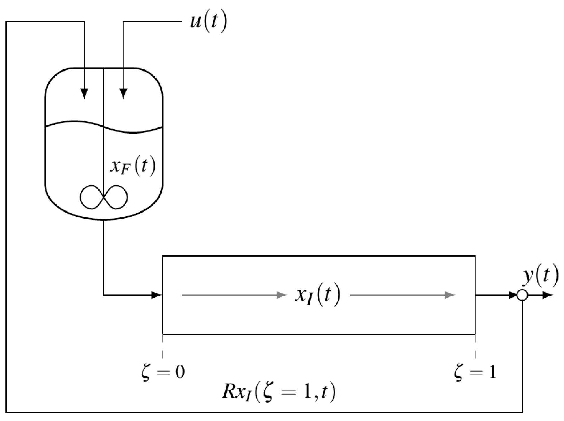
2.1. System Representation

Consider the following coupled CSTR-tubular reactor configuration as the combination of a lumped and parabolic distributed parameter system. This setting is used for some chemical processes (see, e.g., [33]), and can be represented as follows (Figure 1):

The mentioned process can be described by the following coupled ODE-PDE system of equations on domain $\{t\in {\Re }^{+},\zeta \in [0,1]\}$ with algebraic coupled boundaries and initial condition:

$$\begin{array}{c}{\displaystyle \frac{d{x}_F\left(t\right)}{dt}}=a_1{x}_F\left(t\right)+a_{2}u\left(t\right)+R{x}_I(1,t)\hfill \\ {\displaystyle \frac{\partial x_I(\zeta ,t)}{\partial t}}=D{\displaystyle \frac{{\partial }^2{x}_I(\zeta ,t)}{\partial {\zeta }^2}}-v{\displaystyle \frac{\partial x_I(\zeta ,t)}{\partial \zeta }}+\psi x_I(\zeta ,t)+f\left(\zeta \right)d\left(t\right)\hfill \\ x_F\left(0\right)=x_I(\zeta ,0)=1\hfill \\ x_I(0,t)=x_F\left(t\right)\hfill \\ {\displaystyle \frac{\partial x_I(\zeta ,t)}{\partial \zeta }}{|}_{\begin{array}{c}\zeta =1\end{array}}=0\hfill \\ y\left(t\right)=x_I(1,t)\hfill \end{array}$$

(1)

where the second order linear parabolic PDE corresponds to convection-diffusion reactor. The transport of a property $x_I(\zeta ,t)\in L^2(0,1)$ - $L^2(0,1)$ is a Hilbert space—through the tubular reactor, given with the inner product ($<·,·>$), ($L^2(\Omega ;Z)$, $<h,f>={\displaystyle {\int }_{\Omega }<h\left(z\right),f\left(z\right){>}_{Z}dz}$), the ODE indicates the dynamics of the variable $x_F\in \Re$ within the CSTR. $\zeta \in [0,1]$ is the position and $t\ge 0$ is the time variable. $\psi \in \Re$ and $a_1\in \Re$ are the constant values responsible for the consumption or generation of $x_I(\zeta ,t)$ and $x_F\left(t\right)$, respectively. $R\in {\Re }^{+}$ refers to the recycle factor in the system and is considered to be a bounded parameter ($0\le R\le 1$). $v\in {\Re }^{+}$, $D\in {\Re }^{+}$ are the constant transport velocity and diffusion-constant, respectively. $a_2\in \Re$ is a constant number, and $u\left(t\right)$$\in \Re$ represents the system input. $f\left(\zeta \right)$ and $d\left(t\right)$ represent a known disturbance which may present in the tubular reactor and can express changes in unit operations, such as temperature. $d\left(t\right)$ is considered to be a step function and $f\left(\zeta \right)$ is given as follows:

$$f\left(\zeta \right)=\left\{\begin{array}{cc}0\hfill & 0\le \zeta <y_I\hfill \\ k_I\hfill & y_I\le \zeta \le 1\hfill \end{array}\right.$$

(2)

where $y_I$ and $k_I$ are constant values. Here, the linear coupled finite-infinite-dimensional system can be rewritten by the following state-space equations:

$$\begin{array}{c}\dot{x}\left(t\right)=Ax\left(t\right)+Bu\left(t\right)+Md\left(t\right)\hfill \\ y\left(t\right)=Cx(\zeta ,t)\hfill \end{array}$$

(3)

where x is state representing both finite and infinite part of the process $\left(x=\left[\begin{array}{c}{x}_F=x\left(t\right)\\ x_I=x(\zeta ,t)\end{array}\right]\right)$. For the sake of simplicity in the paper, index F refers to the finite part of the system (ODE), while index I indicates the infinite part (PDE). A is defined as a linear operator $\mathfrak{L}\left(X\right)$ (where X is a real space $\Re \oplus L^2(0,1)$), such that $D\left(A\right)=\{x\in X:x_F\in \Re$, $x_I\left(\zeta \right)\in L^2(0,1)$| $x_I\left(\zeta \right)$, ${\displaystyle \frac{dx}{d\zeta }}$ are absolutely continuous, $x_I\left(0\right)=x_F$ and ${\displaystyle \frac{dx(\zeta =0)}{d\zeta }}=0\}$. $B=\left[\begin{array}{c}{a}_2\\ 0\end{array}\right]$ is the linear input operator $\mathfrak{L}(\Re ,X)$, $M=\left[\begin{array}{c}0\\ f\left(\zeta \right)\end{array}\right]$ is the linear disturbance input operator and C=$\left[\begin{array}{cc}0& {\displaystyle {\int }_0^1\delta (\zeta -1)(.)d\zeta }\end{array}\right]$ is the linear output operator.

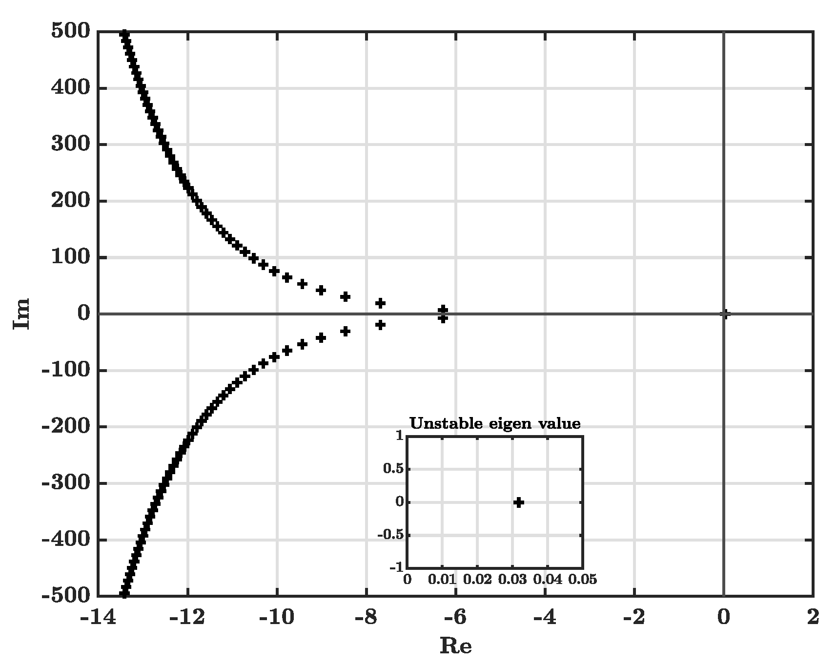
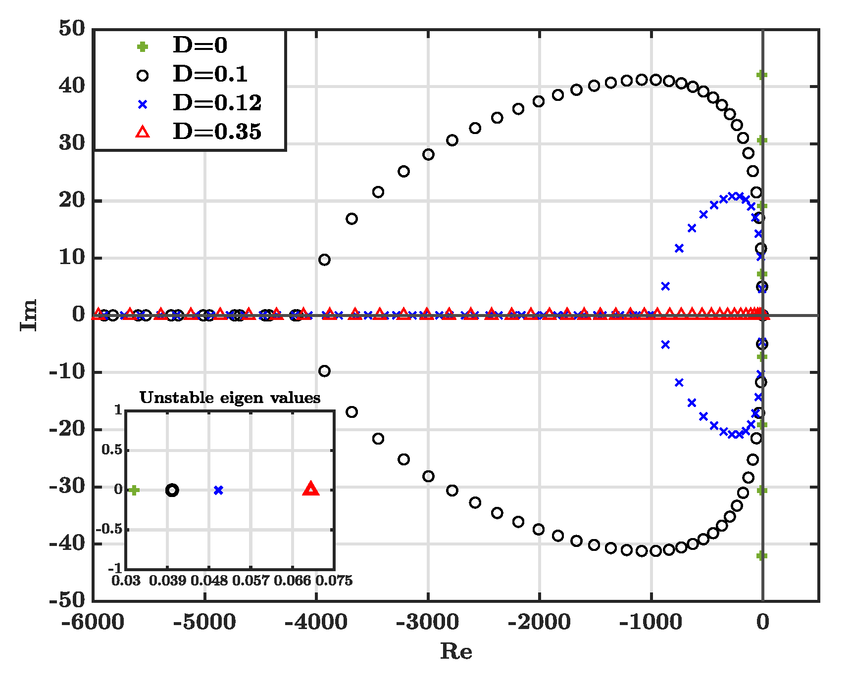
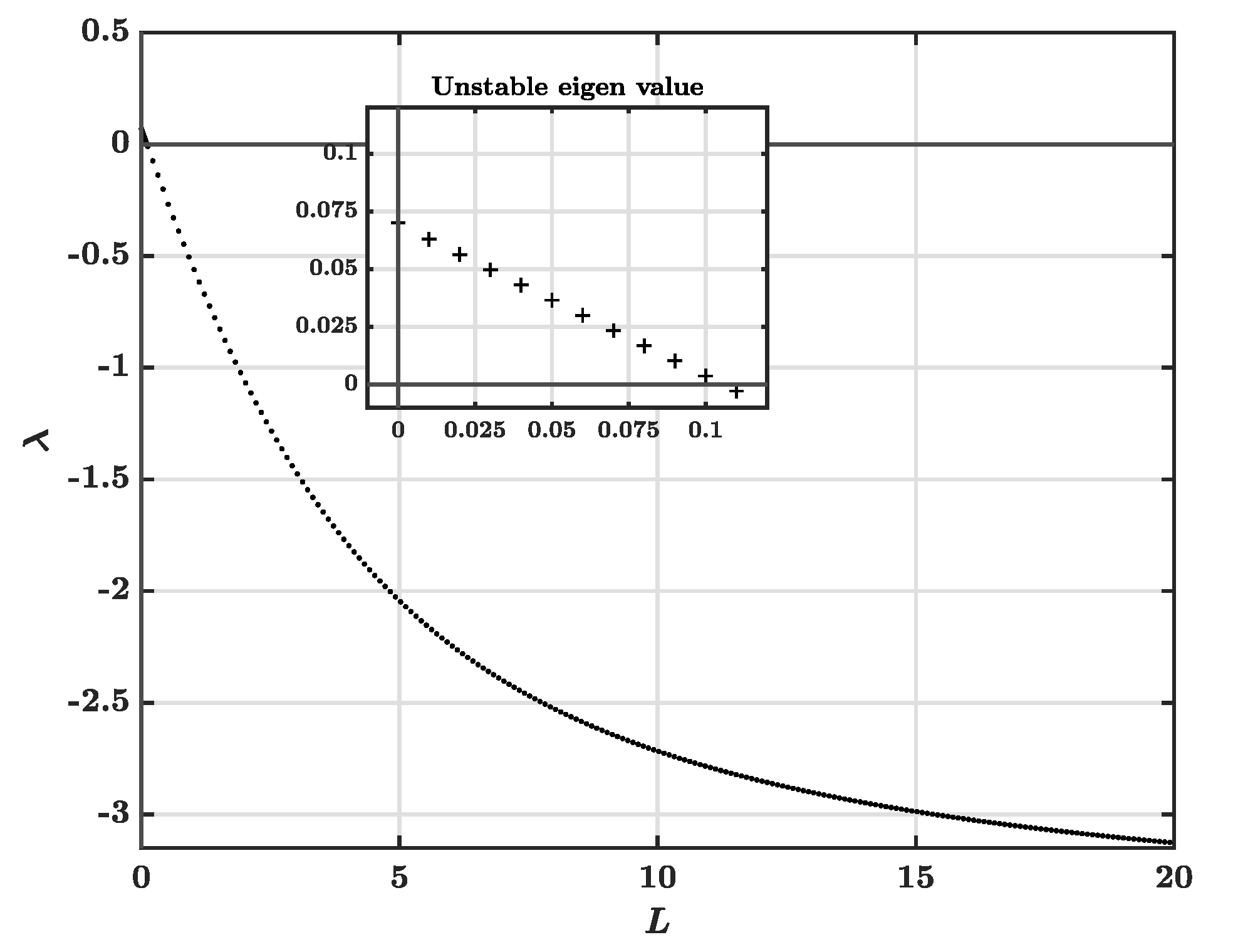
2.2. Open-Loop Stability

The generality of the ensuing design can be established by performing the stability analysis of the target system given by Equation (1). The eigenvalue problem for the open-loop ($u\left(t\right)=0$) unstable coupled ODE-PDE system is defined as below:

$$A\Phi =\lambda \Phi$$

(4)

where :

$$A=\left[\begin{array}{cc}{A}_F=a_1& R{(·)}_I{|}_{\zeta =1}\\ 0& A_I=-v{\displaystyle \frac{\partial {(·)}_I}{\partial \zeta }}+D{\displaystyle \frac{{\partial }^2{(·)}_I}{\partial {\zeta }^2}}+\psi {(·)}_I\end{array}\right],\Phi \left(\zeta \right)=\left[\begin{array}{c}{\Phi }_F\\ {\Phi }_I\left(\zeta \right)\end{array}\right]$$

(5)

$\lambda$ and $\Phi$ are the eigenvalues and eigenfunctions, respectively. The boundary conditions are given by

$${\Phi }_I(\zeta =0)={\Phi }_F,{\displaystyle \frac{d{\Phi }_I\left(\zeta \right)}{d\zeta }}{|}_{\begin{array}{c}\zeta =1\end{array}}=0.$$

(6)

After some simple manipulation and using the boundary conditions defined by Equation (6) in Equation (4), one gets the following:

$$\begin{array}{c}{\displaystyle \frac{d^2{\Phi }_I}{d{\zeta }^2}}-{\displaystyle \frac{v}{D}}{\displaystyle \frac{d{\Phi }_I}{d\zeta }}-{\displaystyle \frac{(\lambda -\psi )}{D}}{\Phi }_I=0\end{array}$$

(7a)

$$\begin{array}{c}{\Phi }_I(\zeta =0)={\Phi }_F=-{\displaystyle \frac{R{\Phi }_I(\zeta =1)}{a_1-\lambda }},{\displaystyle \frac{d{\Phi }_I}{d\zeta }}{|}_{\zeta =1}=0\end{array}$$

(7b)

$\lambda$ and ${\Phi }_I\left(\zeta \right)$ are found numerically from Equation (7a). The solution of Equation (4) with the set of parameters $R=0.55$, $v=1.8$ and consumption of the desired component in both CSTR and dispersive tubular reactor ($\psi =-1$ and $a_1=-0.25$), shows that most eigenvalues have negative real parts and there is only one unstable eigenvalue in the system (see Figure 2 and Figure 3). To explore the effects of diffusion (D) on eigenvalues placement, several values for diffusion were considered. By analyzing Figure 3, with the same conditions, one can notice that as diffusivity increases, the distribution will shift from complex eigenvalues to the real ones.

In this particular chemical engineering system, with the boundary conditions mentioned above, the instability of the coupled ODE-PDE system present with the value assigned for R. As will be discussed in Section 5 by canceling the unstable mode under model predictive control, the stabilization of the system is addressed.

3. Discrete Representation

3.1. Discrete Operators

In this section, the Cayley-Tustin time discretization is applied, which maps the mentioned coupled ODE-PDE system from continuous-time to a discrete one, preserving all energy properties with the feature of no spatial discretization. The discrete version of Equation (3) with sampling time $\Delta t$ can be represented as follows:

$$\begin{array}{c}{x}_{k+1}=A_d{x}_k+B_d{u}_k+M_d{d}_k\hfill \\ y_k=C_d{x}_k+D_d{u}_k+N_d{d}_k\hfill \end{array}$$

(8)

$\delta =2/\Delta t$ and ($A_d$, $B_d$, $C_d$, $D_d$,$M_d$, $N_d$) are the linear discrete operators defined by:

$$\left[\begin{array}{ccc}{A}_d& B_d& M_d\\ C_d& D_d& N_d\end{array}\right]=\left[\begin{array}{ccc}-I+2\delta {\left[\delta -A\right]}^{-1}& \sqrt{2\delta }{\left[\delta -A\right]}^{-1}B& \sqrt{2\delta }{\left[\delta -A\right]}^{-1}M\\ \sqrt{2\delta }C{\left[\delta -A\right]}^{-1}& C{\left[\delta -A\right]}^{-1}B& C{\left[\delta -A\right]}^{-1}M\end{array}\right]$$

(9)

where $\delta =2/\Delta t$, and ${\left[\delta -A\right]}^{-1}=R(\delta ,A)$ is given as the resolvent operator of A in Equation (5). It should be mentioned that the discrete operators are found by replacing s with $\delta$ in $R(s,A)$ . In order to find the resolvent operator, one may easily apply Laplace transform to the set of Equations (1):

$${\displaystyle \frac{\partial }{\partial \zeta }}\underset{X(\zeta ,s)}{\underbrace{\left[\begin{array}{c}{x}_I(\zeta ,s)\\ {\displaystyle \frac{\partial x_I(\zeta ,s)}{\partial \zeta }}\end{array}\right]}}=\underset{P}{\underbrace{\left[\begin{array}{cc}0& 1\\ {\displaystyle \frac{s-\psi }{D}}& {\displaystyle \frac{v}{D}}\end{array}\right]}}\left[\begin{array}{c}{x}_I(\zeta ,s)\\ {\displaystyle \frac{\partial x_I(\zeta ,s)}{\partial \zeta }}\end{array}\right]+\underset{H}{\underbrace{\left[\begin{array}{c}0\\ -{\displaystyle \frac{x_I(\zeta ,0)}{D}}\end{array}\right]}}$$

(10)

Since P is a constant matrix, one can calculate $e^{P\zeta }$ with the Laplace inverse transform ($L^{-1}\left\{{[sI-P]}^{-1}\right\}$). Therefore, the solution of the mentioned system $\left({\displaystyle X(\zeta ,s)=e^{P\zeta }X(0,s)+{\int }_0^{\zeta }{e}^{P(\zeta -\eta )}Hd\eta }\right)$ can be expressed as follows:

$$\left[\begin{array}{c}{x}_I(\zeta ,s)\\ {\displaystyle \frac{\partial x_I(\zeta ,s)}{\partial \zeta }}\end{array}\right]=\left[\begin{array}{cc}{e}_1\left(\zeta \right)& e_2\left(\zeta \right)\\ e_3\left(\zeta \right)& e_4\left(\zeta \right)\end{array}\right]\left[\begin{array}{c}{x}_I(0,s)\\ {\displaystyle \frac{\partial x_I(0,s)}{\partial \zeta }}\end{array}\right]+\left[\begin{array}{c}{b}_1\left(\zeta \right)\\ b_2\left(\zeta \right)\end{array}\right].$$

(11)

After applying the boundary conditions $\left(x_I(\zeta =0,s)=x_F\left(s\right),\frac{\partial x_I(\zeta =1,s)=0}{\partial \zeta }\right)$ to Equation (11), the discrete operators are obtained and have the following form:

$$A_d(·)=-\left[\begin{array}{c}{(·)}_F\\ {(·)}_I\end{array}\right]+2\delta \left[\begin{array}{cc}{R}_{FF}& R_{FI}\\ R_{IF}& R_{II}\end{array}\right]\left[\begin{array}{c}{(·)}_F\\ {(·)}_I\end{array}\right]$$

(12)

$$B_d=\sqrt{2\delta }\left[\begin{array}{c}{R}_{FF}B\\ R_{IF}B\end{array}\right];M_d=\sqrt{2\delta }\left[\begin{array}{c}{R}_{FI}f\left(\zeta \right)\\ R_{II}f\left(\zeta \right)\end{array}\right]$$

(13)

$$C_d=\sqrt{2\delta }\left[\begin{array}{cc}{R}_{IF}{|}_{\zeta =1}& R_{II}{|}_{\zeta =1}\end{array}\right]\left[\begin{array}{c}{(·)}_F\\ {(·)}_I\end{array}\right]$$

(14)

$$D_d=\left[R_{IF}B\right]{|}_{\zeta =1};N_d=\left[R_{II}f\left(\zeta \right)\right]{|}_{\zeta =1}$$

(15)

with the following components:

$$\begin{array}{c}{R}_{FF}{(·)}_F=\left({\displaystyle \frac{{\displaystyle \frac{{(·)}_F}{R}}}{{\displaystyle \frac{\delta -a_1}{R}}-f_3^{\left(1\right)}}}\right),R_{FI}{(·)}_I=\left({\displaystyle \frac{b_1^{\left(1\right)}-{\displaystyle \frac{e_2^{\left(1\right)}{b}_2^{\left(1\right)}}{e_4^{\left(1\right)}}}}{{\displaystyle \frac{\delta -a1}{R}}-f_3^{\left(1\right)}}}\right)\hfill \\ R_{IF}{(·)}_F\left(\zeta \right)=f_3\left(\zeta \right)\left({\displaystyle \frac{\frac{{(·)}_F}{R}}{{\displaystyle \frac{\delta -a_1}{R}}-f_3^{\left(1\right)}}}\right)\hfill \\ R_{II}{(·)}_I\left(\zeta \right)=f_3\left(\zeta \right)\left({\displaystyle \frac{b_1^{\left(1\right)}-\frac{e_2^{\left(1\right)}{b}_2^{\left(1\right)}}{e_4^{\left(1\right)}}}{{\displaystyle \frac{\delta -a_1}{R}}-f_3^{\left(1\right)}}}\right)-{\displaystyle \frac{e_2^{\left(1\right)}{b}_2^{\left(1\right)}}{e_4^{\left(1\right)}}}+b_1\hfill \\ R_{FF}B=f_3\left(\zeta \right)\left({\displaystyle \frac{a_2}{{\displaystyle \frac{{(\delta -a_1)}^2}{R}}-f_3^{\left(1\right)}(\delta -a_1)}}\right)+{\displaystyle \frac{a_2}{\delta -a_1}}\hfill \\ R_{IF}B\left(\zeta \right)=f_3\left(\zeta \right)\left({\displaystyle \frac{{\displaystyle \frac{a_2}{R}}}{{\displaystyle \frac{\delta -a_1}{R}}-f_3^{\left(1\right)}}}\right),R_{FI}f\left(\zeta \right)=\left({\displaystyle \frac{k_1^{\left(1\right)}-{\displaystyle \frac{e_2^{\left(1\right)}{k}_2^{\left(1\right)}}{e_4^{\left(1\right)}}}}{{\displaystyle \frac{\delta -a1}{R}}-f_3^{\left(1\right)}}}\right)\hfill \\ R_{II}f\left(\zeta \right)=f_3\left(\zeta \right)\left({\displaystyle \frac{k_1^{\left(1\right)}-\frac{e_2^{\left(1\right)}{k}_2^{\left(1\right)}}{e_4^{\left(1\right)}}}{{\displaystyle \frac{\delta -a_1}{R}}-f_3^{\left(1\right)}}}\right)-{\displaystyle \frac{e_2^{\left(1\right)}{k}_2^{\left(1\right)}}{e_4^{\left(1\right)}}}+k_1\hfill \end{array}$$

(16)

in above equations $e_1\left(\zeta \right),e_2\left(\zeta \right),e_3\left(\zeta \right),e_4\left(\zeta \right),b_1\left(\zeta \right),b_2\left(\zeta \right),k_1\left(\zeta \right),k_2\left(\zeta \right)$ and $f_3\left(\zeta \right)$ are defined by the following expressions:

$$\begin{array}{c}{e}_1\left(\zeta \right)=e^{\frac{m\zeta }{2}}\left(cosh\left(\frac{h\zeta }{2}\right)-\frac{sinh\left(\frac{h\zeta }{2}\right)m}{h}\right)\hfill \\ e_2\left(\zeta \right)={\displaystyle \frac{2sinh\left(\frac{h\zeta }{2}\right)e^{\frac{m\zeta }{2}}}{h}}\hfill \\ e_3\left(\zeta \right)={\displaystyle \frac{2\left(\frac{\delta -\psi }{D}\right)sinh\left(\frac{h\zeta }{2}\right)e^{\frac{m\zeta }{2}}}{h}}\hfill \\ e_4\left(\zeta \right)=e^{\frac{m\zeta }{2}}\left(cosh\left(\frac{h\zeta }{2}\right)+\frac{sinh\left(\frac{h\zeta }{2}\right)m}{h}\right)\hfill \\ {\displaystyle b_1\left(\zeta \right)={\int }_0^{\zeta }{f}_1(\zeta ,\eta ){(·)}_{I}d\eta }\hfill \\ f_1(\zeta ,\eta )={\displaystyle \frac{-2e^{\frac{\left(\zeta -\eta \right)m}{2}}sinh\left(\frac{h(\zeta -\eta )}{2}\right)}{Dh}}\hfill \\ {\displaystyle k_1\left(\zeta \right)={\int }_0^{\zeta }{f}_1(\zeta ,\eta )f\left(\zeta \right)d\eta }\hfill \\ {\displaystyle b_2\left(\zeta \right)={\int }_0^{\zeta }{f}_2(\zeta ,\eta ){(·)}_{I}d\eta }\hfill \\ f_2(\zeta ,\eta )=-{\displaystyle \frac{e^{\frac{\left(\zeta -\eta \right)m}{2}}}{D}}\left[cosh\left({\displaystyle \frac{h(\zeta -\eta )}{2}}\right)+{\displaystyle \frac{sinh\left(\frac{h(\zeta -\eta )}{2}\right)m}{h}}\right]\hfill \\ {\displaystyle k_2\left(\zeta \right)={\int }_0^{\zeta }{f}_2(\zeta ,\eta )f\left(\zeta \right)d\eta }\hfill \\ m={\displaystyle \frac{v}{D}}\hfill \\ h=\sqrt{{\left({\displaystyle \frac{v}{D}}\right)}^2+4\left({\displaystyle \frac{\delta -\psi }{D}}\right)}\hfill \\ f_3\left(\zeta \right)=e_1\left(\zeta \right)-{\displaystyle \frac{e_2\left(\zeta \right)e_3^{\left(1\right)}}{e_4^{\left(1\right)}}}\hfill \end{array}$$

(17)

where $e_1^{\left(1\right)}$, $e_2^{\left(1\right)}$, $e_3^{\left(1\right)}$, $e_4^{\left(1\right)}$, $b_1^{\left(1\right)}$, $b_2^{\left(1\right)}$, $k_1^{\left(1\right)}$, $k_2^{\left(1\right)}$, $f_1^{\left(1\right)}$, $f_2^{\left(1\right)}$ and $f_3^{\left(1\right)}$ are the corresponding terms calculated at $\zeta$ = L = 1.

3.2. Discrete Adjoint Operators

The adjoint operators are required for developing the model predictive control. The expressions for adjoints $(A_d^{*},B_d^{*})$ of the discrete operators $(A_d,B_d)$ are written in the following form:

$$A_d^{*}(·)=-\left[\begin{array}{c}{(·)}_F\\ {(·)}_I\end{array}\right]+2\delta \left[\begin{array}{cc}{R}_{FF}^{*}& R_{IF}^{*}\\ R_{FI}^{*}& R_{II}^{*}\end{array}\right]\left[\begin{array}{c}{(·)}_F\\ {(·)}_I\end{array}\right]$$

(18)

$$B_d^{*}=\sqrt{2\delta }{\left[\begin{array}{c}{\left(R_{FF}B\right)}^{*}\\ {\left(R_{IF}B\right)}^{*}\end{array}\right]}^T$$

(19)

the components of the adjoint operators are computed based on the definition ($<A_d\Phi ,{\Psi }^{★}>=<\Phi ,A_d^{★}{\Psi }^{★}>$) and results in following operators:

$$\begin{array}{c}{R}_{FF}^{*}{(·)}_F=R_{FF}{(·)}_F\hfill \\ {\displaystyle R_{IF}^{*}{(·)}_I={\int }_0^L\left[{\displaystyle \frac{e_1-{\displaystyle \frac{e_2{e}_3^{\left(1\right)}}{e_4^{\left(1\right)}}}}{\delta -a_1-R{f}_3^{\left(1\right)}}}\right]{(·)}_{I}d\zeta }\hfill \\ R_{FI}^{*}{(·)}_F\left(\zeta \right)=\left({\displaystyle \frac{f_1^{\left(1\right)}}{{\displaystyle \frac{\delta -a_1}{R}}-f_3^{\left(1\right)}}}-{\displaystyle \frac{{\displaystyle \frac{e_2^{\left(1\right)}{f}_2^{\left(1\right)}}{e_4^{\left(1\right)}}}}{{\displaystyle \frac{\delta -a_1}{R}}-f_3^{\left(1\right)}}}\right){(·)}_F\hfill \\ R_{II}^{*}{(·)}_I\left(\zeta \right)=\left({\displaystyle -f_2^{\left(1\right)}{\int }_0^L\left[{\displaystyle \frac{e_2^{\left(1\right)}}{e_4^{\left(1\right)}\left(\delta -a_1-R{f}_3^{\left(1\right)}\right)}}{f}_3\left(\eta \right)+{\displaystyle \frac{e_2\left(\eta \right)}{e_4^{\left(1\right)}}}\right]{(·)}_{I}d\eta }\right)+\hfill \\ \left({\displaystyle f_1^{\left(1\right)}{\int }_0^L\left[{\displaystyle \frac{f_3\left(\eta \right)}{\left(\delta -a_1-R{f}_3^{\left(1\right)}\right)}}\right]{(·)}_{I}d\eta +{\int }_{\zeta }^L{f}_1(\eta ,\zeta ){(·)}_{I}d\eta }\right)\hfill \\ {\left(R_{FF}B\right)}^{*}{(·)}_F=\left({\displaystyle \frac{a_2{f}_3^{\left(1\right)}}{{\displaystyle \frac{{(\delta -a_1)}^2}{R}}-f_3^{\left(1\right)}(\delta -a_1)}}+{\displaystyle \frac{a_2}{\delta -a_1}}\right){(·)}_F\hfill \\ {\displaystyle {\left(R_{IF}B\right)}^{*}{(·)}_I=\left({\displaystyle \frac{{\displaystyle \frac{a_2}{R}}}{{\displaystyle \frac{\delta -a_1}{R}}-f_3^{\left(1\right)}}}\right){\int }_0^L\left[e_1\left(\zeta \right)-{\displaystyle \frac{e_3^{\left(1\right)}{e}_2\left(\zeta \right)}{e_4^{\left(1\right)}}}\right]{(·)}_{I}d\zeta }\hfill \end{array}$$

(20)

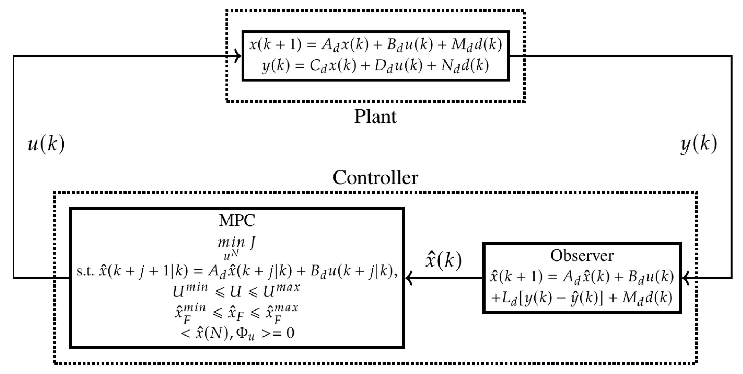
4. Luenberger Observer Design

In a real process system controller realization, having access to all the state variables cannot be feasible, especially when DPS are considered. In order to address this issue in the design of the model predictive control, the Luenberger observer is introduced for reconstruction of the state variables by taking the output measurement into account. First, the design of observer for the coupled parabolic PDE-ODE system in the continuous setting is considered. Then, the continuous observer gain is transferred into the discrete one using Cayley-Tustin discretization. The Luenberger observer has the form given by:

$$\begin{array}{c}\dot{\widehat{x}}(\zeta ,t)=A\widehat{x}(\zeta ,t)+Bu\left(t\right)+L_c[y\left(t\right)-\widehat{y}\left(t\right)]+f\left(\zeta \right)d\left(t\right)\hfill \\ \widehat{y}\left(t\right)=C\widehat{x}(\zeta ,t)\hfill \end{array}$$

(21)

where $L_c$=$\left[\begin{array}{c}{L}_F\\ L_I\left(\zeta \right)\end{array}\right]$ is the continuous observer gain. By subtracting Equation (21) from its general form $\left(\dot{x}(\zeta ,t)=Ax(\zeta ,t)+Bu\left(t\right)\right)$, one can get the dynamics of the observer error as follows:

$$\begin{array}{c}\dot{\widehat{e}}(\zeta ,t)=(A-L_{c}C)\widehat{e}\left(t\right),\widehat{e}\left(0\right)\ne 0\hfill \end{array}$$

(22)

the design of the observer is relied on choosing $L_c$ such that the state estimation error dynamics given by Equation (22) is stable. Hence, the stability of the observer can be ensured by analyzing the eigenvalues problem of the observer error:

$$(A-L_{c}C)\Phi =\lambda \Phi$$

(23)

which results in following equation and boundary conditions:

$$\begin{array}{c}{\displaystyle \frac{d^2{\Phi }_I}{d{\zeta }^2}}-{\displaystyle \frac{v}{D}}{\displaystyle \frac{d{\Phi }_I}{d\zeta }}-{\displaystyle \frac{(\lambda -\psi )}{D}}{\Phi }_I={\displaystyle \frac{L_I\left(\zeta \right)}{D}}{\Phi }_I(\zeta =1)\end{array}$$

(24a)

$$\begin{array}{c}{\Phi }_I(\zeta =0)={\Phi }_F=-{\displaystyle \frac{(L_F-R){\Phi }_I(\zeta =1)}{a_1-\lambda }},{\displaystyle \frac{d{\Phi }_I}{d\zeta }}{|}_{\zeta =1}=0.\end{array}$$

(24b)

Figure 4 shows the eigenvalues placement for different values of $L_c$=$\left[\begin{array}{c}{L}_F\\ L_I\left(\zeta \right)\end{array}\right]$. It should be emphasized that in the eigenvalue problem, although a spatially varying $L_I\left(\zeta \right)$ could be chosen, a constant value throughout the whole spatial domain ($L_I\left(\zeta \right)=L$) is considered and the same value assigned for the finite part ($L_F=L$). It can be seen that as the value of $L_c$ increases, the unstable real eigenvalue is shifted to the left side (the stable region). Therefore, as depicted in Figure 4 for $L_c>0.1$ the stability of the error dynamics will be ensured by having only negative eigenvalues. Here, the resolvent is used to compute the corresponding discrete observer gain from the continuous one [34]:

$$L_d=\sqrt{2\delta }\left[\begin{array}{cc}{R}_{FF}& R_{FI}\\ R_{IF}& R_{II}\end{array}\right]\left[\begin{array}{c}{L}_F\\ L_I\left(\zeta \right)\end{array}\right].$$

(25)

Therefore, the reconstructed state in the discrete setting can be expressed as:

$$\begin{array}{c}{\widehat{x}}_{k+1}=A_d{\widehat{x}}_k+B_d{u}_k+L_d(y_k-{\widehat{y}}_k)+M_d{d}_k\hfill \\ {\widehat{y}}_k=C_d{\widehat{x}}_k+D_d{u}_k+N_d{d}_k,y_k=C_d{x}_k+D_d{u}_k+N_d{d}_k\hfill \end{array}$$

(26)

5. Model Predictive Control for Linear Coupled ODE-PDE System

5.1. Optimization Problem

The linear discrete-time model dynamics represented in Equations (12)–(20) is used in the formulation of the model predictive control for the coupled CSTR and tubular reactor system. The MPC developed in [31] regarding linear time invariant systems for the finite-dimensional setting is extended to infinite-dimensional one. In order to achieve this purpose, the following objective function should be minimized at each sampling time (k) to design the regulator of the coupled ODE-PDE system:

$$\begin{array}{c}{\displaystyle \underset{u^N}{min}J=\sum _{j=0}^{\infty }<\widehat{x}(k+j|k),Q\widehat{x}(k+j|k)>+<u(k+j+1|k),Fu(k+j+1|k)>}\hfill \\ s.t.\widehat{x}(k+j+1|k)=A_d\widehat{x}(k+j|k)+B_{d}u(k+j|k),\hfill \\ u^{min}⩽u(k+j|k)⩽u^{max},\hfill \\ {\widehat{x}}_F^{min}⩽{\widehat{x}}_F(k+j|k)⩽x_F^{max},\hfill \\ <\widehat{x}(k+N),{\Phi }_u>=0\hfill \end{array}$$

(27)

where $\widehat{x}=$$\left[\begin{array}{c}{\widehat{x}}_F\\ {\widehat{x}}_I\end{array}\right]$ refers to the reconstructed state, F is a positive definite operator, Q=$\left[\begin{array}{c}{Q}_F\\ Q_I\end{array}\right]$ represents positive semidefinite spatial operator associated with the state of coupled ODE-PDE system and the indices, ($k+j$) and ($k+j+1|k$), for both input and state variable, indicate current and future time, respectively. In order to get the finite horizon objective function, one can assume zero input beyond the control horizon (i.e., $u(k+N+1|k)=0$) by taking the terminal penalty term into an account. The result takes the following form:

$$\begin{array}{c}{\displaystyle \underset{u^N}{min}J=\sum _{j=0}^{N-1}<\widehat{x}(k+j|k),Q\widehat{x}(k+j|k)>+<u(k+j+1|k),Fu(k+j+1|k)>}\hfill \\ +<\widehat{x}(k+N|k),\overline{Q}\widehat{x}(k+N|k)>\hfill \\ s.t.\widehat{x}(k+j+1|k)=A_d\widehat{x}(k+j|k)+B_{d}u(k+j|k),\hfill \\ u^{min}⩽u(k+j|k)⩽u^{max},\hfill \\ {\widehat{x}}_F^{min}⩽{\widehat{x}}_F(k+j|k)⩽x_F^{max},\hfill \\ <\widehat{x}(k+N),{\Phi }_u>=0.\hfill \end{array}$$

(28)

After simple algebraic manipulation, the following finite-dimensional quadratic optimization problem is obtained:

$$\begin{array}{c}\underset{U}{min}J=U^{T}HU+2U^{T}P\widehat{x}\left(k\right|k)+<\widehat{x}\left(k\right|k),\overline{Q}\widehat{x}\left(k\right|k)>\hfill \end{array}$$

(29a)

where $\overline{Q}$ is terminal state penalty operator. The above equation is subjected to the following constraints:

$$\begin{array}{c}\left\{\begin{array}{c}1.U^{min}⩽U⩽U^{max}\hfill \\ 2.{\widehat{x}}_F^{min}⩽{\widehat{x}}_F⩽{\widehat{x}}_F^{max}\hfill \\ 3.<\widehat{x}\left(N\right),{\Phi }_u>=0\hfill \end{array}\right.\end{array}$$

(29b)

where $U={\left[\begin{array}{ccccc}u(k+1|k)& u(k+2|k)& u(k+3|k)& \cdots & u(k+N|k)\end{array}\right]}^T$ and $(H,P)$ are computed as below:

$$\begin{array}{c}H=\left[\begin{array}{cccc}{B}_d^{*}\overline{Q}{B}_d+F& B_d^{*}{A}_d^{*}\overline{Q}{B}_d& \cdots & B_d^{*}{A_d^{*}}^{N-1}\overline{Q}{B}_d\\ B_d^{*}\overline{Q}{A}_d{B}_d& B_d^{*}\overline{Q}{B}_d+F& \cdots & B_d^{*}{A_d^{*}}^{N-2}\overline{Q}{B}_d\\ ⋮& ⋮& \ddots & ⋮\\ B_d^{*}\overline{Q}{A}_d^{N-1}{B}_d& B_d^{*}\overline{Q}{A}_d^{N-2}{B}_d& \cdots & B_d^{*}\overline{Q}{B}_d+F\end{array}\right],\hfill \\ P=\left[\begin{array}{c}{B}_d^{*}\overline{Q}{A}_d\\ B_d^{*}\overline{Q}{A}_d^2\\ ⋮\\ B_d^{*}\overline{Q}{A}_d^N\end{array}\right].\hfill \end{array}$$

(30)

The model predictive control scheme used on the coupled ODE-PDE system is illustrated in Figure 5. As can be seen, the full state feedback is needed for the MPC scheme, which is going to be given by the reconstructed states from the observer.

5.2. Terminal State Penalty Operator

The terminal state penalty term, the operator $\overline{Q}$=$\left[\begin{array}{c}{\overline{Q}}_F\\ {\overline{Q}}_I\end{array}\right]$, can be found from the solution of the following discrete Lyapunov equation:

$$A_d^{*}\overline{Q}{A}_d-\overline{Q}=-Q.$$

(31)

The above solution of the discrete Lyapunov equation based on Cayley-Tustin method is the same unique solution of $\overline{Q}$ in Equation (31) in continuous setting ($A^{*}\overline{Q}+\overline{Q}A=-Q$) [35]. Since the solution of $\overline{Q}$ cannot be obtained directly; in other words, because of the necessity of using integral operators coming from discrete operators for calculating $\overline{Q}$, the procedure followed here is to connect the discrete and continuous Lyapunov equations. Here, one can rewrite the continuous Lyapunov equation in the following format [36]:

$$<A{x}_1,\overline{Q}{x}_2>+<\overline{Q}{x}_1,A{x}_2>=-<x_1,Q{x}_2>.$$

(32)

By considering $x_1={\widehat{\Phi }}^m$ and $x_2={\widehat{\Psi }}^m$ and using the fact that ${\lambda }^m$ and ${\widehat{\Psi }}^m$ are the eigenvalue and eigen function of the system (i.e., $A{\widehat{\Phi }}^m={\lambda }^m{\widehat{\Phi }}^m$), the equation leads to:

$$<{\lambda }^m{\widehat{\Phi }}^m,\overline{Q}{\widehat{\Psi }}^m>+<\overline{Q}{\widehat{\Phi }}^m,{\lambda }^m{\widehat{\Psi }}^m>={\lambda }^m<{\widehat{\Phi }}^m,\overline{Q}{\widehat{\Psi }}^m>+{\lambda }^m<\overline{Q}{\widehat{\Phi }}^m,{\widehat{\Psi }}^m>=-<{\widehat{\Phi }}^m,Q{\widehat{\Psi }}^m>$$

(33)

$\overline{Q}$ is a bounded symmetric operator $(D\left(A^{*}\right)=D\left(A\right))$ and it is self-adjoint (see [36]) which implies $<{\widehat{\Phi }}^m,\overline{Q}{\widehat{\Psi }}^m>=<\overline{Q}{\widehat{\Phi }}^m,{\widehat{\Psi }}^m>={\overline{Q}}^m$, accordingly the following simplified equation is achieved:

$${\overline{Q}}^m={\displaystyle \frac{-<{\widehat{\Phi }}^m,Q{\widehat{\Psi }}^m>}{2{\lambda }^m}}.$$

(34)

Finally, the solution of the continuous Lyapunov equation gives the expression for the infinite part (PDE) of the terminal state penalty operator (${\overline{Q}}_I$) which can be expressed as below:

$${\displaystyle {\overline{Q}}_I{(·)}_I=\sum _{m=0}^{\infty }\frac{-<{{\widehat{\Phi }}_I}^m,Q_I{{\widehat{\Psi }}_I}^m>}{2{\lambda }^m}<{(·)}_I,{{\widehat{\Psi }}_I}^m>{{\widehat{\Phi }}_I}^m}$$

(35)

where ${\widehat{\Phi }}_I^m$ and ${\widehat{\Psi }}_I^m$ refer to the normalized eigenfunction and adjoint eigenfunction of infinite part of the system, respectively. In Equation (35), the summation is computed for increasing number of different eigenvalues, until the applied operator converges to a constant value. In this work the first 20 eigen modes are considered in the simulation. For the finite part (ODE), $A_F=A_F^{*}=a_1$. According to Lyapunov equation, ${\overline{Q}}_F$ is easily obtained and given by the following expression:

$${\overline{Q}}_F{(·)}_F=\frac{Q_F}{2a_1}{(·)}_F$$

(36)

5.3. Stability Constraint

Based on the definition of a positive definite operator, it is possible to show that $\overline{Q}$ is a positive operator if only the stable nodes are taken into account [36]. In order to guarantee stabilization of the system, a stability constraint is applied in the optimization problem and is represented by an equality constraint [35]. It is assumed that the controller will gain stabilization by rejecting the unstable modes. Hence, this condition can be written as below:

$$<\widehat{x}\left(N\right),{\Phi }_u>=0$$

(37)

where ${\Phi }_u$ refer to unstable eigenfunctions associated with positive eigenvalues. The corresponding equality constraint, which cancels the unstable modes at end of the horizon, is constructed as follows:

$$\begin{array}{c}\left[\begin{array}{ccc}<A_d^{N-1}{B}_d,{\Phi }_u>& \cdots & <B_d,{\Phi }_u>\end{array}\right]U\hfill \\ =-<A_d^N\widehat{x}\left(k\right|k),{\Phi }_u>.\hfill \end{array}$$

(38)

If there is a feasible input sequence given by optimization problem, the above equality constraint is satisfied for the constrained convex optimization problem given by Equation (29a). Therefore, stabilization can be obtained, and the unstable modes will be canceled by end of the horizon. Here, due to the feasibility of the optimization represented by constrained quadratic problem in the zero-disturbance case, feasibility implies stability and optimal stabilizability. This extension is based on the well-known results from the finite-dimensional theory [30,31].

6. Simulation Results

In this section, the simulation study is performed for the proposed controller of the coupled ODE-PDE system. First, the design of the observer is discussed in the discrete setting with reconstruction of states in an open-loop condition by using Cayley-Tustin method, then the performance of the ensuing Model Predictive Control is demonstrated and compared with the open-loop response.

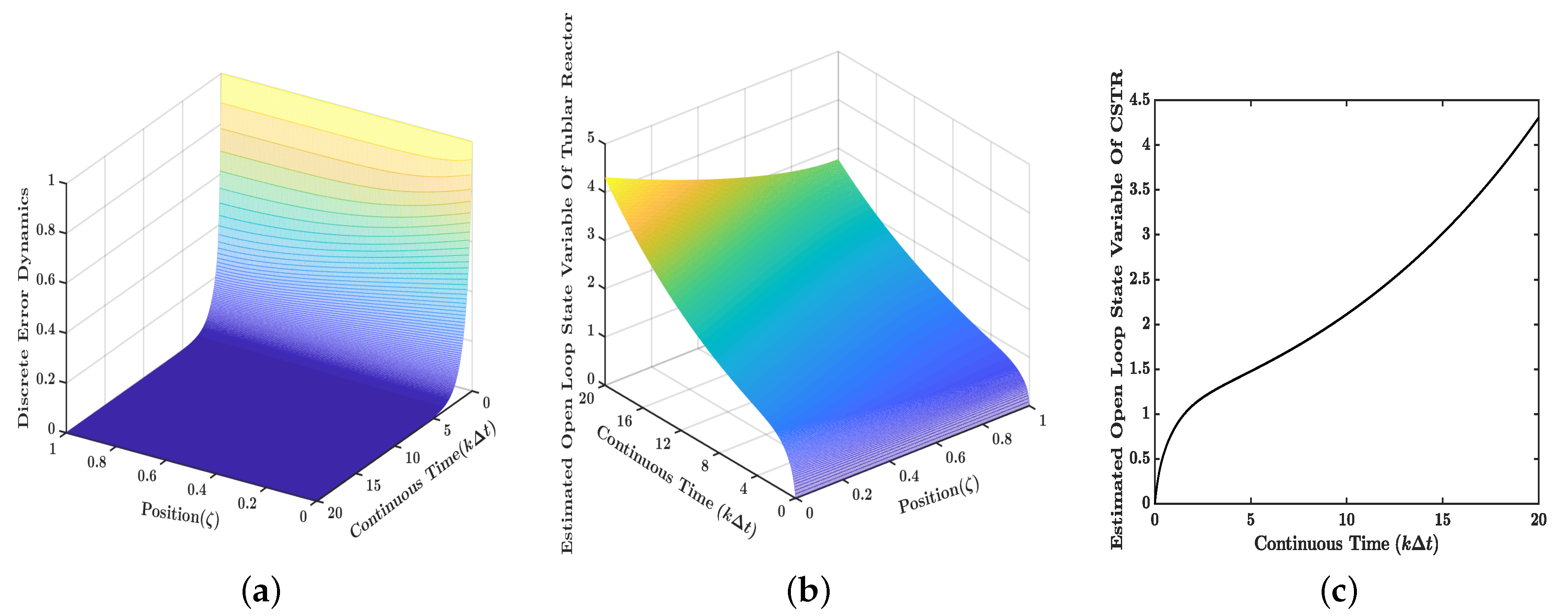
6.1. Observer Design and Open-Loop Response

Based on Equations (8)–(13), one can reconstruct the dynamics of the discrete representation for both finite and infinite parts of the system with the set of parameters given in

Table 1. Parameter values used in numerical simulation.

Parameters	Values
v	$1.8$
F	1
D	$0.35$
$a_1$	$-0.25$
$\psi$	$-1$
$a_2$	1
R	$0.5$
$u^{min}$	$-0.09$
$u^{max}$	0
${x_F}^{min}$	0
${x_F}^{max}$	$0.65$

. As discussed in Section 4, to guarantee the stability of the observer, $L_c=5$ is chosen as the observer gain. By using Equation (25) the discrete version of the corresponding observer gain is computed. The initial conditions for the mentioned observer and original system are considered to be constants in the entire space, ${\widehat{x}}_0=0$ and $x_0=1$, respectively. In simulation $\Delta t=0.04$ is considered which implies $\delta =50$ and for numerical integration $\Delta z=0.005$ is chosen. Then, according to Equation (26), the reconstructed state is obtained, and the corresponding error dynamics is evaluated. As shown in Figure 6a, the dynamics of the observer error converges to zero, which means the developed observer has a good performance. Hence, in the case of a realistic system, the Model Predictive Control can be applied using just the output measurement.

As discussed in Section 2.2 regarding the instability of the coupled ODE-PDE system, Figure 6b demonstrates the space-time evolution of the tubular reactor ($x_I(\zeta ,t)$) for $0\le t\le 20$ which grows unbounded as expected. Following this, the corresponding dynamics of the CSTR ($x_F\left(t\right)$) with pertaining initial condition is depicted in Figure 6c.

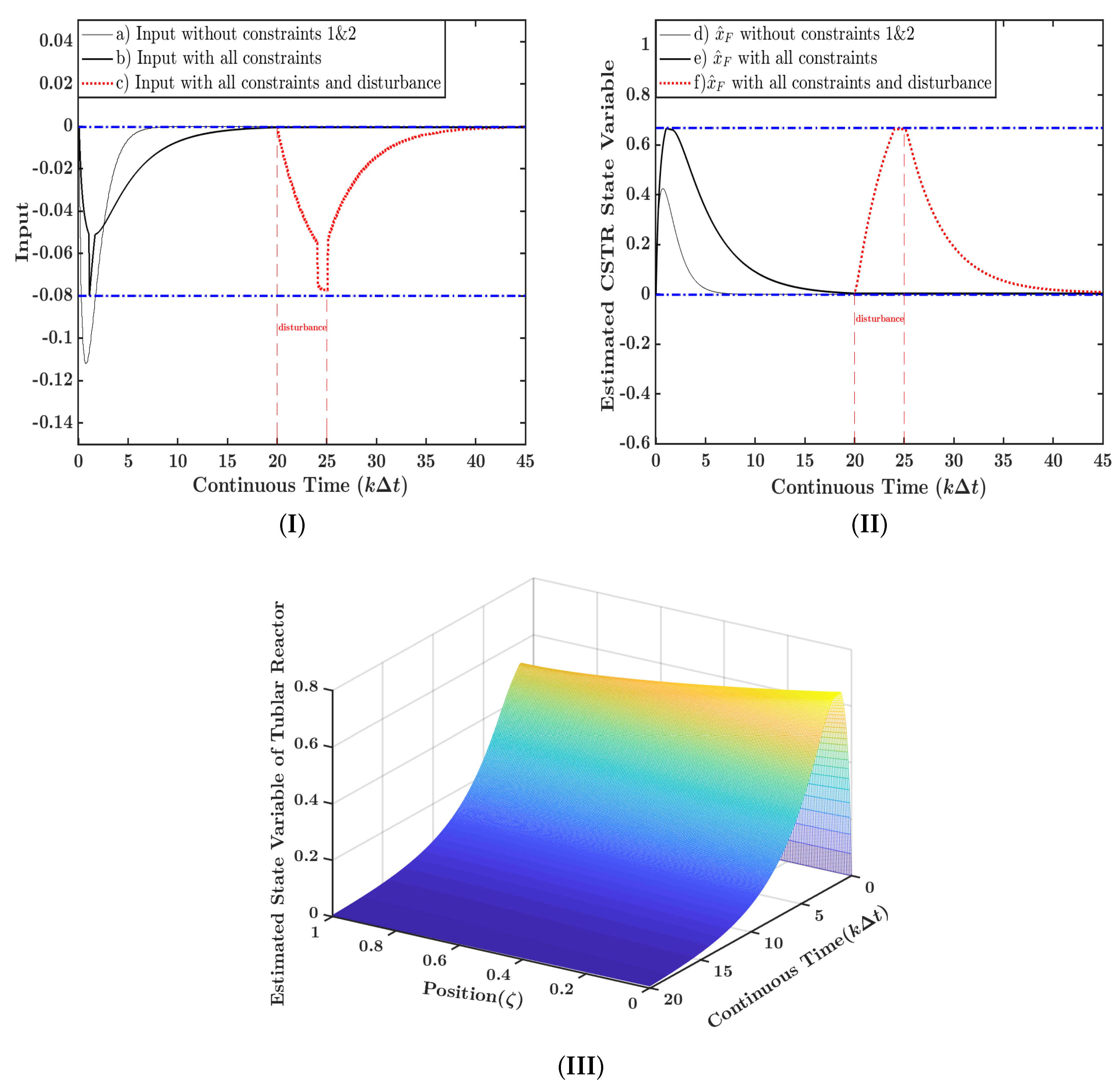
6.2. MPC Implementation

In this part, based on the scheme represented by Figure 5, the successful application of the proposed constrained model predictive controller is demonstrated on the basis of Cayley-Tustin time discretization with optimization problem described by Equations (27)–(38). The implementation of the system under model predictive control with and without constraints (see Equation (29b)) in time domain $0\le t\le 20$ is shown in Figure 7(b)) and Figure 7(d)). By choosing $Q{}_F$ = 2.5, $Q{}_I\left(\zeta \right)$ = $1.5$ and N = 65 for the MPC control horizon, it is possible to see that the controller is able to comply with the input and states constraints (dash-dotted lines) imposed into the coupled ODE-PDE system. Moreover, regarding the instability of the system, as described in Section 5.3, one can notice that the stability constraint is also fulfilled by canceling the unstable mode at end of the horizon (see Figure 7(c)).

On the other hand, in order to provide a comparison of the dynamics of scalar variable $x_F$ in CSTR with input and state constraints, the simulation is performed again to justify two scenarios, for the first one only stability constraint is considered in the MPC algorithm while in the second one all constraints (stability, input and state) are present. Figure 7(d)) and Figure 7(e)) show this analogy with corresponding control actions given by Figure 7(a)) and Figure 7(b)). As expected in the first setting, the CSTR dynamics is faster compared to the latter case as no state/input constraints need to be satisfied.

Another simulation has been performed to explore the behavior of the MPC algorithm for handling the mentioned constraints, the step disturbance is applied through the infinite part of the system (tubular reactor) for $20\le t\le 25$. The idea here is to examine the performance of the MPC algorithm for stabilization and the state/input constrains satisfaction. $y_I=0.5$ and $k_I=0.6$ are chosen as the parameters in Equation (2) describing spatial varying function $f\left(\zeta \right)$. Figure 7(c)) and Figure 7(f)) verify the good performance of MPC for handling the constraints when the disturbance is present. By analyzing Figure 7(c)), one can notice that after the step disturbance is applied, the state variable of the CSTR stays at the upper limit ($x_F^{max}$) until $t=25$, then decreases and once again goes back to zero (at $t=45$) based on the control action given by Figure 7(c)).

7. Conclusions

In this contribution, the design of a model predictive controller and discrete observer for a coupled ODE-PDE system was investigated. In particular, the lumped and distributed system were coupled by the boundaries, with the manipulated variable acting on the ODE. The system stability characteristics were first analyzed by studying the system’s eigenvalues. A discrete representation of the system was necessary in the controller design; thus, the Cayley-Tustin time discretization was applied, preserving the original system characteristics. An unstable operation condition was considered, and the MPC and observer design had to take this into account. To develop the discrete observer, the design in the continuous-time setting was first derived, then the discrete observer was obtained based on the continuous gain. The MPC was designed to obtain the optimal control sequence while handling input constraints and stabilizing the system using a terminal constraint. Finally, numerical simulations were shown to present the performance of the controller in the closed loop. As expected, the controller was able to achieve stabilization, while handling the constraints. If a disturbance is made, the controller can deal with the effects made in the system while satisfying the constraints.

The constrained optimal control design for the class of parabolic and hyperbolic PDEs, which guarantees the system stability and handling both input and state constraints will be an extension to be addressed in future studies.

References

1. Ray, W. Advanced Process Control; McGraw-Hill: New York, NY, USA, 1981; p. 1984. [Google Scholar]
2. Muske, K.R.; Rawlings, J.B. Model predictive control with linear models. AIChE J. 1993, 39, 262–287. [Google Scholar] [CrossRef]
3. Rawlings, J.B. Tutorial overview of model predictive control. IEEE Control Syst. Mag. 2000, 20, 38–52. [Google Scholar]
4. Eaton, J.W.; Rawlings, J.B. Model-Predictive Control of Chemical Processes. Chem. Eng. Sci. 1992, 47, 705–720. [Google Scholar] [CrossRef]
5. Richalet, J.; Rault, A.; Testud, J.; Papon, J. Model predictive heuristic control: Applications to industrial processes. Automatica 1978, 14, 413–428. [Google Scholar] [CrossRef]
6. Shang, H.; Forbes, J.F.; Guay, M. Model Predictive Control for Quasilinear Hyperbolic Distributed Parameter Systems. Ind. Eng. Chem. Res. 2004, 43, 2140–2149. [Google Scholar] [CrossRef]
7. Armaou, A.; Christofides, P. Dynamic optimization of dissipative PDE systems using nonlinear order reduction. Chem. Eng. Sci. 2002, 57, 5083–5114. [Google Scholar] [CrossRef]
8. Krstic, M.; Smyshlyaev, A. Backstepping boundary control for first-order hyperbolic PDEs and application to systems with actuator and sensor delays. Syst. Control Lett. 2008, 57, 750–758. [Google Scholar] [CrossRef]
9. Oh, M.; Pantelides, C. A Modelling and Simulation Language for Combined Lumped and Distributed Parameter Systems. Comput. Chem. Eng. 1996. [Google Scholar] [CrossRef]
10. Mohammadi, L.; Aksikas, I.; Dubljevic, S.; Forbes, J.F. Optimal boundary control of coupled parabolic PDE–ODE systems using infinite-dimensional representation. J. Process Control 2015, 33, 102–111. [Google Scholar] [CrossRef]
11. Moghadam, A.A.; Aksikas, I.; Dubljevic, S.; Forbes, J.F. Boundary optimal (LQ) control of coupled hyperbolic PDEs and ODEs. Automatica 2013, 49, 526–533. [Google Scholar] [CrossRef]
12. Susto, G.A.; Krstic, M. Control of PDE–ODE cascades with Neumann interconnections. J. Frankl. Inst. 2010, 347, 284–314. [Google Scholar] [CrossRef]
13. Hasan, A.; Aamo, O.M.; Krstic, M. Boundary observer design for hyperbolic PDE–ODE cascade systems. Automatica 2016, 68, 75–86. [Google Scholar] [CrossRef]
14. Tang, S.; Xie, C. State and output feedback boundary control for a coupled PDE–ODE system. Syst. Control Lett. 2011, 60, 540–545. [Google Scholar] [CrossRef]
15. Krstic, M.; Smyshlyaev, A. Boundary Control of Pdes: A Course on Backstepping Designs; Society for Industrial and Applied Mathematics: Philadelphia, PA, USA, 2008. [Google Scholar]
16. Meglio, F.D.; Argomedo, F.B.; Hu, L.; Krstic, M. Stabilization of coupled linear heterodirectional hyperbolic PDE–ODE systems. Automatica 2018, 87, 281–289. [Google Scholar] [CrossRef] [Green Version]
17. Mayne, D.; Rawlings, J.; Rao, C.; Scokaert, P. Constrained model predictive control: Stability and optimality. Automatica 2000, 36, 789–814. [Google Scholar] [CrossRef]
18. Chen, H.; Allgöwer, F. Nonlinear Model Predictive Control Schemes with Guaranteed Stability. In Nonlinear Model Based Process Control; Springer Netherlands: Dordrecht, The Netherlands, 1998. [Google Scholar] [CrossRef]
19. García, C.E.; Prett, D.M.; Morari, M. Model predictive control: Theory and practice—A survey. Automatica 1989, 25, 335–348. [Google Scholar] [CrossRef]
20. Ito, K.; Kunisch, K. Receding horizon optimal control for infinite dimensional systems. ESAIM Control. Optim. Calc. Var. 2002, 8, 741–760. [Google Scholar] [CrossRef] [Green Version]
21. Dubljevic, S.; El-Farra, N.H.; Mhaskar, P.; Christofides, P.D. Predictive control of parabolic PDEs with state and control constraints. Int. J. Robust Nonlinear Control 2006, 16, 749–772. [Google Scholar] [CrossRef]
22. Liu, L.; Huang, B.; Dubljevic, S. Model predictive control of axial dispersion chemical reactor. J. Process Control 2014, 24, 1671–1690. [Google Scholar] [CrossRef]
23. Dubljevic, S.; Christofides, P.D. Predictive control of parabolic PDEs with boundary control actuation. Chem. Eng. Sci. 2006, 61, 6239–6248. [Google Scholar] [CrossRef]
24. Bonis, I.; Xie, W.; Theodoropoulos, C. A linear model predictive control algorithm for nonlinear large-scale distributed parameter systems. AIChE J. 2012, 58, 801–811. [Google Scholar] [CrossRef]
25. Ai, L.; San, Y. Model Predictive Control for Nonlinear Distributed Parameter Systems based on LS-SVM. Asian J. Control 2013, 15, 1407–1416. [Google Scholar] [CrossRef]
26. Kazantzis, N.; Kravaris, C. Energy-predictive control: A new synthesis approach for nonlinear process control. Chem. Eng. Sci. 1999, 54, 1697–1709. [Google Scholar] [CrossRef]
27. Åström, K.J.; Wittenmark, B. Computer-Controlled Systems: Theory and Design, 2nd ed.; Prentice-Hall, Inc.: Upper Saddle River, NJ, USA, 1990. [Google Scholar]
28. Havu, V.; Malinen, J. The Cayley Transform as a Time Discretization Scheme. Numer. Funct. Anal. Optim. 2007, 28, 825–851. [Google Scholar] [CrossRef] [Green Version]
29. Hairer, E.; Lubich, C.; Wanner, G. Geometric Numerical Integration: Structure-Preserving Algorithms for Ordinary Differential Equations, 2nd ed.; Springer: Berlin/Heidelberg, Germany, 2006. [Google Scholar] [CrossRef] [Green Version]
30. Mayne, D.Q. Model predictive control: Recent developments and future promise. Automatica 2014, 50, 2967–2986. [Google Scholar] [CrossRef]
31. Rawlings, J.; Mayne, D.; Diehl, M. Model Predictive Control: Theory, Computation, and Design; Nob Hill Publishing: Santa Barbara, CA, USA, 2017. [Google Scholar]
32. Scokaert, P.O.M.; Mayne, D.Q.; Rawlings, J.B. Suboptimal model predictive control (feasibility implies stability). IEEE Trans. Autom. Control 1999. [Google Scholar] [CrossRef] [Green Version]
33. Fogler, H.S. Elements of Chemical Reaction Engineering; Prentice-Hall: Upper Saddle River, NJ, USA, 2005. [Google Scholar]
34. Ozorio Cassol, G.; Dubljevic, S. Discrete Output Regulator Design for the linearized Saint-Venant-Exner model. Unpublished work.
35. Xu, Q.; Dubljevic, S. Linear Model Predictive Control for Transport-Reaction Processes. AIChE J. 2017, 63. [Google Scholar] [CrossRef]
36. Curtain, R.; Zwart, H. An Introduction to Infinite Dimensional Linear Systems Theory; Springer: Berlin, Germany, 1995. [Google Scholar]
Figure 1. CSTR-tubular reactor system with recycle stream.
Mathematics 08 00711 g001
Figure 2. Eigenvalues distribution for unstable coupled ODE-PDE system when there is no diffusion within the tubular reactor.
Mathematics 08 00711 g002
Figure 3. Effects of diffusivity within the dispersive reactor on the eigenvalues placement for unstable coupled ODE-PDE system.
Mathematics 08 00711 g003
Figure 4. Shifting the unstable eigenvalue of the observer for different values of the observer gain.
Mathematics 08 00711 g004
Figure 5. Representation of the closed loop.
Mathematics 08 00711 g005
Figure 6. (a) Evolution of the discrete error dynamics with the value L c = 5 for observer gain; (b) The estimated state profile evolution ( x I ( ζ , k ) ) through dispersive tubular reactor constructed on the basis of discrete-time coupled ODE-PDE system in an open-loop condition; (c) Dynamics reconstruction of the scalar variable within the CSTR in an open-loop condition.
Mathematics 08 00711 g006
Figure 7. (I) (a), (b) and (c) demonstrate the comparison between input profiles under model predictive control law: with and without input/state constraints, with constraints and with disturbance for 20 t 25 ; (II) (d), (e) and (f) denote reconstructed dynamics of the scalar variable within the CSTR under model predictive law: with and without input/state constraints, with constraints and with disturbance for 20 t 25 ; (III) Evolution of the stabilized spatial profile for the tubular reactor with all constraints.
Mathematics 08 00711 g007