Abstract
The main object of this paper is to develop an alternative construction for the bimodal skew-normal distribution. The construction is based upon a study of the mixture of skew-normal distributions. We study some basic properties of this family, its stochastic representations and expressions for its moments. Parameters are estimated using the maximum likelihood estimation method. A simulation study is carried out to observe the performance of the maximum likelihood estimators. Finally, we compare the efficiency of the new distribution with other distributions in the literature using a real data set. The study shows that the proposed approach presents satisfactory results.
1. Introduction
The skew-normal distribution was introduced by Azzalini [1], typically denoted as , with asymmetry parameter , so that becomes the standard normal distribution. Hence, has a density function given by
with and where and denote, respectively, the density and distribution functions of the distribution. Some well known facts about this distribution are
where and are asymmetry and kurtosis coefficients, respectively. From (3) it is well known that
Henze [2] developed the stochastic representation for the skew-normal density and computed its odd moments. The stochastic representation and some more general representations for skew models are also discussed in Azzalini [3]. Arnold et al. [4] make use of the above results to develop truncations of the normal model. Pewsey [5] studied inference problems faced by the skew-normal model with some general results, especially consequences of the singularity of the Fisher information matrix (FIM) in the vicinity of symmetry. Gupta and Chen [6] developed a goodness of fit test. Reliability studies for the skew-normal model were developed by Gupta and Brown [7]. Univariate extensions to the skew-normal model are studied in Arellano-Valle et al. [8], Azzalini [9], Gómez et al. ([10,11]), [12], etc.
When it is necessary to model data with more than one mode, mixtures of distributions are always used. The importance of such studies rests on the fact that these models present computational difficulties due to identifiability problems. One major motivation of this paper is to develop models than can be seen as alternative parametric models to replace the use of mixtures of distributions, as these present estimation problems from either classical or Bayesian points of view ([13,14]). Bimodal distributions generated from skew distributions can be found in Azzalini and Capitanio [15], Ma and Genton [16], Arellano-Valle et al. [17], Kim [18], Lin et al. ([19,20]), Elal-Olivero et al. [21], Arnold et al. [22], Arellano-Valle et al. [23], Elal-Olivero [24], Gómez et al. [25], Arnold et al. [26], Braga et al. [27], Venegas et al. [28], Shah et al. [29], Gómez-Déniz et al. [30], Esmaeili et al. [31], Imani and Ghoreishi [32], Maleki et al. [33], etc. The main object of this paper is to study the properties of the bimodal skew-normal model introduced by Elal-Olivero et al. [21]. In particular, we derive results related to stochastic representation of the distribution and density function; this makes it simple to derive distributional moments and inferences by maximum likelihood (ML) estimation, among other quantities. The paper is organized as follows. Section 2 develops a bimodal normal distribution, its basic properties, representation, moments and moment generating function. Section 3 develops a skew-normal bimodal distribution, its basic properties, stochastic representation, moments and moment generating function. In Section 4, we perform a small scale simulation study of the ML estimators for parameters. A real data application is discussed in Section 5, which illustrates the usefulness of the proposed model. Conclusions and future work are presented in Section 6.
2. Preliminaries
2.1. Bimodal Normal Distribution
Definition 1.
If the random variable X has density function
where ϕ is the density, we say that X follows a bimodal normal distribution(see Elal-Olivero [24]) which is denoted by .
Remark 1.
If with its density, then is bimodal. This can be verified by noticing that , and it follows that it reaches its minimum value at and maximum value at and . Notice that the maximum value is the same; this fact will play en important role in defining a more flexible model by adding an extra parameter which will control the height at the modes.
For the sake of completeness, some important results derived in Elal-Olivero [24] are presented below.
- If and and are the corresponding distribution and the moment generating functions then
- (a)
- (b)
- (c)
- Let X and U be independent random variables with and U such that . If then .
2.2. Bimodal Normal Distribution with Shape Parameter
Definition 2.
If random variable X has density given by
where ϕ is the density of the distribution, we say that X is distributed according to the bimodal normal distribution with parameter α which we denote by .
Remark 2.
Some basic properties are shown in the following. Under the assumption that and that is the density function of X, then
- (a)
- (b)
- is symmetric around zero ∀
- (c)
- As , then .
- (d)
- is bimodal ∀ > where and are the points where the density reaches its maximum.
- (e)
- is unimodal .
Proposition 1.
If then the cumulative distribution and the moment generating function (MGF), denoted by and respectively, are given by:
- ;
Proof.
Follows directly from the corresponding definitions. □
The next result presents a stochastic representation for the distribution.
Proposition 2.
Let X and Y be independent random variables such that and . If then
Proof.
Using moments definition,
which agrees with the MGF of derived above. □
Proposition 3.
Let . Then for the moments are given by: and
Proof.
Follows directly from moment definition. □
Hence, the kurtosis coefficient is given by Recall that the kurtosis coefficient is given by
given that the even moments are zero and and , which proves the result.
Remark 3.

Considering that the model is unimodal for , Table 1 shows the variation for the kurtosis coefficient as parameter α ranges the interval.
Table 1.
Kurtosis values for model.
3. Bimodal Asymmetric Distribution
We start by dealing first with the extension of the ordinary normal bimodal distribution.
3.1. One-Parameter Bimodal Skew-Normal Distribution
Definition 3.
If the random variable X is distributed according to the density function
then we say that it is distributed according to the bimodal skew normal distribution with parameter λ which we denote by .
Figure 1 depicts examples of the bimodal skew-normal (BSN) distribution given in Equation (8) for different values of parameter .
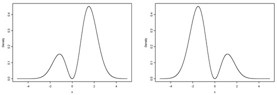
Figure 1.
Density with parameter (left) and (right).
Proposition 4.
Let , then .
Proof.
Let , then, for , it follows that
Differentiating this last expression we conclude the proof by showing that
□
Remark 4.
The density function , behaves like the density function of the bimodal normal model by the perturbation function . We note that the heights at the modes for a bimodal symmetric distribution are the same. However, for an asymmetric distribution the heights at the modes are not the same as shown in the next proposition.
Proposition 5.
Let , . Moreover, let and () be the points at which the function reaches its the maximum value. Then,
- (a)
- If then
- (b)
- If then .
Proof.
If (symmetric case) then with and .
Suppose now that ; it should then be required that and .
Hence, ∀, and, in particular, . On the other hand, for the symmetric case, it is known that and given that , it follows that
The case is proved similarly. □
Proposition 6.
Let , and be the distribution functions of the random variables , respectively, and the density function of Y. Therefore,
with .
Proof.
Let
the distribution function of the random variable . Integrating by parts, with and , it follows that and , so that
□
Proposition 7.
Let and with MGF and , respectively. Then,
with and .
Proof.
We have
Integrating by parts, with and , it follows that
and so that
□
3.2. Two-Parameter Bimodal Skew-Normal Distribution
Definition 4.
If the density function of a random variable X is such that
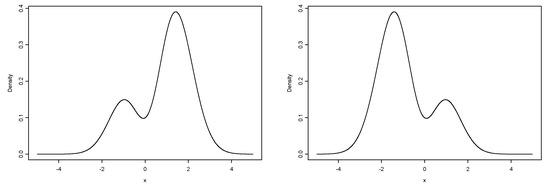
then we say that X is distributed as the bimodal skew-normal distribution(see Elal-Oliviero et al. [21]) with parameters λ and α, which we denote by . Figure 2 depicts examples of the BSN distribution given in Equation (9) for different values of parameters λ and α.
Figure 2.
Density function for with and (left); and (right).
Remark 5.
It is already known that changes in parameter λ lead to changes in values (heights) of the density of the model, that is, in . By incorporating the extra parameter α in the density , corresponding to the model, as α ranges in the interval the density changes from unimodal to bimodal, and vice versa, with great flexibility.
As we mentioned in the introduction, the BSN model was introduced by Elal-Olivero et al. [21] and used for the Bayesian inference. Now we observe that we have constructed it based on a mixture of two distributions; below we study some of its properties, carry out a simulation study to see the behavior of the ML estimators and present an application to a real data set.
Proposition 8.
Let , so that the following properties hold:
- (a)
- If then
- (b)
- If then
- (c)
- If then
- (d)
- If then
- (e)
- Let , , and . Then,Proof.For , it follows thatwhich upon differentiation leads to:□
- (f)
- Let , and . ThenProof.We note that the density for the model can be seen as a mixture between the and models. □
Proposition 9.
Let , and and be the distribution function for the random variables W and Y respectively and the density function Y. Then,
Proof.
Let be the distribution function of the random variable X, where . Then, the result follows by noticing that
□
Proposition 10.
Let and , and let, and be the moment generating functions for the random variables W and Y, respectively; then,
with , and
Proof.
The result follows by noticing that
□
Remark 6.
The properties for the model presented next follow from general properties of the model presented in Azzalini [3] where is a symmetric (around zero) density function, G is a unidimensional (symmetric) distribution function such that exists and is an even function.
- 1.
- A stochastic representation for the model. Let and be independent random variables and defineThen .
- 2.
- Invariance perturbation property.If and then are identically distributed.
Remark 7.
The moments of the model can be computed easily, separating even from odd moments.
- 1.
- Considering anti-perturbation invariance, the even moments of X and Z are the same, so that with .
- 2.
- For the odd moments, considering that , it follows that:with .where the odd moments can be computed using derivations in Henze [2], leading to:with .
If we denote by and the asymmetry and kurtosis coefficients, respectively, then:
where , with are as given by
Representing the asymmetry for specific values of and by , then the following relation holds:
Table 2.
Possible values of the standardized skewness coefficient.
Table 3.
Possible values of the standardized kurtosis coefficient.
The parameter produces asymmetry in the symmetric model and, in particular when , the asymmetry is reflected in the change of height of the modes of the symmetric bimodal model.
The following proposition shows the identifiability of the model.
Proposition 11.
The model is identifiable.
Proof.
Let fixed. We will prove that if then , for all . Let us assume, for a contradiction, that , for all and fixed. Thus, after some algebraic procedures, we have that , for all . In consequence, is a contradiction of our assumption.
To prove that f is an injective function with respect to parameter , we use an analogous procedure, which concludes the proof. □
Below we show some properties involving conditional distributions and their relations with the model introduced in this paper.
Proposition 12.
If and . Then .
Proof.
The proof follows by noticing that
□
Corollary 1.
If and , then .
Proposition 13.
Let and . Then .
Proof.
□
3.3. Location-Scale Extension
In practical scenarios, it is common to work with the location-scale transformation , where , and , with and . Therefore, the density function for the random variable X, denoted as is given by
Let us assume that is a random sample of size n from the distribution . From (10), the log-likelihood function is given as
where , which is a continuous function of each parameter. Then, differentiating the log-likelihood function, we obtain that the elements of the score vector, , where , are given by
where . Therefore, the ML estimator of is the solution of the system , which must be solved numerically.
4. Simulation Study
In this section we report results of a small scale Monte Carlo simulation study conducted to evaluate the performance of parameter estimation by ML. Results are based on 1000 samples generated from the BSN model for several sample sizes. Use was made of the stochastic representation presented in Remark 6(1) implemented in R software [34]. For each sample generated, the likelihood function was maximized using the optim function of the R software. Given that the Fisher information matrix is singular when in the vicinity of symmetry (), the use of algorithms such as Fisher-Scoring is not advisable. We therefore used the Nelder and Mead [35] algorithm, a direct search method that works satisfactorily for non-differentiable functions.
4.1. Nelder-Mead Method
For each sample size and parameter configuration, the ML estimators were computed leading to an empirical mean and empirical standard deviation (SD). Results are depicted in Table 4 and Table 5. The main conclusion is that estimation was satisfactorily stable for moderate and large sample sizes.
Table 4.
Empirical means and standard deviations for ML estimators using Nelder-Mead method (with and ).
Table 5.
Empirical means and standard deviations for ML estimators using Nelder-Mead method (with and ).
The simulation study also indicated certain difficulties in the estimation approach for situations near singularity, see Table 6 below. Table 6 below reports the results.
Table 6.
Percentage of samples that presented convergence problems.
With , convergence problems were less frequent (), and for , very few cases presented problems.
4.2. Fisher-Scoring Method
Table 7 shows simulation results using the Fisher-Scoring algorithm. It was obtained that for and (and ), for , non-convergence was down to . For some improvement was noted in the convergence rate although the standard error remained large as increased. Parameter recovery was satisfactory even for moderate sample sizes.
Table 7.
Empirical means and standard deviations for ML estimators using Fisher-scoring method (with and ).
5. Application
We next present an application of the BN() model to a real data situation in which comparisons are made with the mixture of normals model and a flexible asymmetric model. We fitted these models to the variable ultrasound weight, i.e., fetus weight before birth, in 500 observations of the variable z = b.weight, which is the ultrasound weight (fetal weight in grams). These data are available at http://www.mat.uda.cl/hsalinas/cursos/2011/R/weight.rar. Given the difference in weight of males and females in the gestation stage, it is clear that these data present bimodality.
The descriptive statistics are given in Table 8, where and denote the asymmetry and kurtosis coefficients respectively.
Table 8.
Summary statistics for variable fetal weight in grams.
The fit of this data set with the BSN model is compared with the fit given by the mixture of two normals (MN) model, and the flexible skew-normal (FSN) model introduced by Ma and Genton [16], for which the respective densities are given by:
where and denote the density and distribution functions of the standard normal distribution, , and . ML estimation, Akaike’s information criterion (AIC) (see Akaike [36]) and Bayesian information criterion (BIC) (see Schwarz [37]) are reported in Table 9.
Table 9.
ML estimates and Akaike’s information criterion (AIC) values for the three models.
Notice that the BSN model presents the best fit (smallest AIC and BIC values). This is also corroborated by Figure 3, which shows the curves corresponding to the fitted models (parameters estimated using the ML approach), overlaid by the data set histogram.
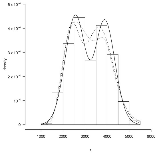
Figure 3.
Models fitted by the ML approach for the fetal weight in grams data set: BSN (solid line), MN (dashed line) and FSN (dotted line).
6. Concluding Remarks
In this paper we have studied further properties of the so called BSN model. Stochastic representations were studied for the model itself and for some sub-models. Derivation of the FIM and verification of its non-singularity is in preparation and will be the subject of a future paper. Satisfactory results are obtained for the BSN model in a real data application. Some additional features of the BSN model are:
- The BSN models present no identifiability problems, as shown by Proposition 11.
- The moments, moment generating function, asymmetry and kurtosis coefficients have closed form expressions.
- The simulation study shows that, although there is a little irregularity in consistency for values , the ML estimators are consistent. This point of irregularity can be explained by the singularity that exists in this point of the information matrix; we will address this situation in a future work.
- We use a model which is a mixture of non-identifiable normal distributions for comparison with the BSN model.
- In the application, two statistical criteria for comparing models were used. The two criteria indicate that the BSN model provides the best fit for these data.
Author Contributions
Conceptualization, D.E.-O., H.B. and H.W.G.; Data curation, J.F.O.-P.; Formal analysis, D.E.-O, J.F.O.-P. and O.V.; Funding acquisition, H.W.G.; Investigation, D.E.-O., O.V. and H.W.G.; Methodology, H.B.; Resources, O.V.; Software, J.F.O.-P.; Writing–original draft, O.V. and H.B. All authors have read and agreed to the published version of the manuscript.
Funding
The research of H.W. Gómez was supported by Grant SEMILLERO UA-2020 (Chile). The research of O. Venegas was supported by Vicerrectoría de Investigación y Postgrado de la Universidad Católica de Temuco, Projecto interno FEQUIP 2019-INRN-03.
Acknowledgments
We acknowledge the referees’ suggestions that helped us improve this work.
Conflicts of Interest
The authors declare no conflict of interest.
References
- Azzalini, A. A class of distributions which includes the normal ones. Scand. J. Stat. 1985, 12, 171–178. [Google Scholar]
- Henze, N. A probabilistic representation of the skew-normal distribution. Scand. J. Stat. 1986, 13, 271–275. [Google Scholar]
- Azzalini, A. Further results on a class of distributions which includes the normal ones. Statistica 1986, 46, 199–208. [Google Scholar]
- Arnold, B.C.; Beaver, R.J.; Groeneveld, R.A.; Meeker, W.Q. The nontruncated marginal of a truncated bivariate normal distribution. Psychometrika 1993, 58, 471–478. [Google Scholar] [CrossRef]
- Pewsey, A. Problems of inference for Azzalini’s skew-normal distribution. J. Appl. Stat. 2000, 27, 859–870. [Google Scholar] [CrossRef]
- Gupta, A.K.; Chen, T. Goodness-of-fit tests for the skew-normal distribution. Commun. Stat. Simula C 2001, 30, 907–930. [Google Scholar]
- Gupta, R.C.; Brown, N. Reliability studies of the skew-normal distribution and its application to a strength-stress model. Commun. Stat. Theory Methods 2001, 30, 2427–2445. [Google Scholar] [CrossRef]
- Arellano-Valle, R.B.; Gómez, H.W.; Quintana, F.A. A New Class of Skew-Normal Distributions. Commun. Stat. Theory Methods 2004, 33, 1465–1480. [Google Scholar] [CrossRef]
- Azzalini, A. The skew-normal distribution and related multivariate families (with discussion). Scand. J. Stat. 2005, 32, 159–188. [Google Scholar] [CrossRef]
- Gómez, H.W.; Salinas, H.S.; Bolfarine, H. Generalized skew-normal models: Properties and inference. Statistics 2006, 40, 495–505. [Google Scholar] [CrossRef]
- Gómez, H.W.; Torres, F.J.; Bolfarine, H. Large-Sample Inference for the Epsilon-Skew-t Distribution. Commun. Stat. Theory Methods 2007, 36, 73–81. [Google Scholar] [CrossRef]
- Venegas, O.; Sanhueza, A.I.; Gómez, H.W. An extension of the skew-generalized normal distribution and its derivation. Proyecciones J. Math. 2011, 30, 401–413. [Google Scholar] [CrossRef]
- McLachlan, G.; Peel, D. Finite Mixture Models; John Wiley & Sons, Inc.: New York, NY, USA, 2000. [Google Scholar]
- Marin, J.M.; Mengersen, K.; Robert, C. Bayesian modeling and inference on mixtures of distributions. In Handbook of Statistics; Elsevier: Amsterdam, The Netherlands, 2005; Volume 25, pp. 459–503. [Google Scholar]
- Azzalini, A.; Capitanio, A. Distributions generate by perturbation of symmetry with emphasis on a multivariate skew-t distribution. J. R. Stat. Soc. Ser. B 2003, 65, 367–389. [Google Scholar] [CrossRef]
- Ma, Y.; Genton, M.G. Flexible class of skew-symmetric distributions. Scand. J. Stat. 2004, 31, 459–468. [Google Scholar] [CrossRef]
- Arellano-Valle, R.B.; Gómez, H.W.; Quintana, F.A. Statistical inference for a general class of asymmetric distributions. J. Stat. Plan. Inference 2005, 128, 427–443. [Google Scholar] [CrossRef]
- Kim, H.J. On a class of two-piece skew-normal distributions. Statistics 2005, 39, 537–553. [Google Scholar] [CrossRef]
- Lin, T.I.; Lee, J.C.; Hsieh, W.J. Robust mixture models using the skew-t distribution. Stat. Comput. 2007, 17, 81–92. [Google Scholar] [CrossRef]
- Lin, T.I.; Lee, J.C.; Yen, S.Y. Finite mixture modeling using the skew-normal distribution. Stat. Sin. 2007, 17, 909–927. [Google Scholar]
- Elal-Olivero, D.; Gómez, H.W.; Quintana, F.A. Bayesian Modeling using a class of Bimodal skew-Elliptical distributions. J. Stat. Plan. Inference 2009, 139, 1484–1492. [Google Scholar] [CrossRef]
- Arnold, B.C.; Gómez, H.W.; Salinas, H.S. On multiple constraint skewed models. Statistics 2009, 43, 279–293. [Google Scholar] [CrossRef]
- Arellano-Valle, R.B.; Cortés, M.A.; Gómez, H.W. An extension of the epsilon-skew-normal distribution. Commun. Stat. Theory Methods 2010, 39, 912–922. [Google Scholar] [CrossRef]
- Elal-Olivero, D. Alpha-Skew-Normal Distribution. Proyecciones J. Math. 2010, 29, 224–240. [Google Scholar] [CrossRef]
- Gómez, H.W.; Elal-Olivero, D.; Salinas, H.S.; Bolfarine, H. Bimodal extension based on the skew-normal distribution with application to pollen data. Environmetrics 2011, 22, 50–62. [Google Scholar] [CrossRef]
- Arnold, B.C.; Gómez, H.W.; Salinas, H.S. A doubly skewed normal distribution. Statistics 2015, 49, 842–858. [Google Scholar] [CrossRef]
- Da Silva Braga, A.; Cordeiro, G.M.; Ortega, E.M.M. A new skew-bimodal distribution with applications. Commun. Stat. Theory Methods 2017, 47, 2950–2968. [Google Scholar] [CrossRef]
- Venegas, O.; Salinas, H.S.; Gallardo, D.I.; Bolfarine, B.; Gómez, H.W. Bimodality based on the generalized skew-normal distribution. J. Stat. Comput. Simul. 2018, 88, 156–181. [Google Scholar] [CrossRef]
- Shah, S.; Chakraborty, S.; Hazarika, P.J. A New One Parameter Bimodal Skew Logistic Distribution and its Applications. arXiv 2019, arXiv:1906.04125. [Google Scholar]
- Gómez-Déniz, E.; Pérez-Rodríguez, J.V.; Reyes, J.; Gómez, H.W. A Bimodal Discrete Shifted Poisson Distribution. A Case Study of Tourists’ Length of Stay. Symmetry 2020, 12, 442. [Google Scholar] [CrossRef]
- Esmaeili, H.; Lak, F.; Alizadeh, M.; Monfared, M.E.D. The Alpha-Beta Skew Logistic Distribution: Properties and Applications. Stat. Optim. Inf. Comput. 2020, 8, 304–317. [Google Scholar] [CrossRef]
- Imani, M.; Ghoreishi, S.F. Bayesian optimization objective-based experimental design. In Proceedings of the 2020 American Control Conference (ACC 2020), Denver, CO, USA, 1–3 July 2020. [Google Scholar]
- Maleki, M.; Wraith, D.; Arellano-Valle, R.B. Robust finite mixture modeling of multivariate unrestricted skew-normal generalized hyperbolic distributions. Stat. Comput. 2019, 29, 415–428. [Google Scholar] [CrossRef]
- R Core Team. R: A Language and Environment for Statistical Computing; R Foundation for Statistical Computing: Vienna, Austria, 2017. [Google Scholar]
- Nelder, J.A.; Mead, R. A simplex algorithm for function minimization. Comput. J. 1965, 7, 308–313. [Google Scholar] [CrossRef]
- Akaike, H. A new look at the statistical model identification. IEEE Trans. Autom. Control. 1974, 19, 716–723. [Google Scholar] [CrossRef]
- Schwarz, G. Estimating the dimension of a model. Ann. Stat. 1978, 6, 461–464. [Google Scholar] [CrossRef]
© 2020 by the authors. Licensee MDPI, Basel, Switzerland. This article is an open access article distributed under the terms and conditions of the Creative Commons Attribution (CC BY) license (http://creativecommons.org/licenses/by/4.0/).