Article

Innovative Platform for Designing Hybrid Collaborative & Context-Aware Data Mining Scenarios

1
Electric, Electronic and Computer Engineering Department, Technical University of Cluj-Napoca, North University Center of Baia Mare, 400114 Cluj-Napoca, Romania
2
HOLISUN, 430397 Baia-Mare, Romania
3
Department of Mathematics and Informatics, Technical University of Cluj-Napoca, North University Center of Baia Mare, 400114 Cluj-Napoca, Romania
*
Author to whom correspondence should be addressed.
Mathematics 2020, 8(5), 684; https://doi.org/10.3390/math8050684
Submission received: 30 March 2020 / Revised: 21 April 2020 / Accepted: 29 April 2020 / Published: 1 May 2020
(This article belongs to the Special Issue Computational Intelligence)

Abstract

:
The process of knowledge discovery involves nowadays a major number of techniques. Context-Aware Data Mining (CADM) and Collaborative Data Mining (CDM) are some of the recent ones. the current research proposes a new hybrid and efficient tool to design prediction models called Scenarios Platform-Collaborative & Context-Aware Data Mining (SP-CCADM). Both CADM and CDM approaches are included in the new platform in a flexible manner; SP-CCADM allows the setting and testing of multiple configurable scenarios related to data mining at once. The introduced platform was successfully tested and validated on real life scenarios, providing better results than each standalone technique—CADM and CDM. Nevertheless, SP-CCADM was validated with various machine learning algorithms—k-Nearest Neighbour (k-NN), Deep Learning (DL), Gradient Boosted Trees (GBT) and Decision Trees (DT). SP-CCADM makes a step forward when confronting complex data, properly approaching data contexts and collaboration between data. Numerical experiments and statistics illustrate in detail the potential of the proposed platform.

1. Introduction

Nowadays, technology allows the storing of larger amounts of data. Having this data analyzed in a proper manner could help us enhance our processes and discover important patterns in data, that would lead to improvements in every domain this knowledge is applied to. Collecting data is a process that is still dependent on different sensors, programs or machines. Any disruption in the functioning of the data provider can result in loss of data or noise in the obtained data. That is a reason why various approaches are the subject of continuous research in the data mining processes.
Han et al. [1] emphasize the need to have different techniques for covering the discrepancies that are brought in the data mining process by the incomplete, noisy or inconsistent data [2]. Stahl et al. [3] use the Pocket Data Mining term to define the collaborative mining of streaming data in mobile and distributed computing environments and propose an architecture in this direction.
Correia et al. [4] also designed a collaborative framework allowing researchers to share the results and their expertise so that these can be further used in other research. Web services were implemented and deployed and were responsible for seeking relevant knowledge among the collaborative web sites. They designed and deployed a prototype for collaborative data mining in the fields of Molecular Biology and Chemoinformatics. In Reference [5], data mining extract rules associate user profile and context features with an eligible set of recommendable points of interest to tourists.
Matei et al. [6,7] proposed for the first time a multi-layered architecture for data mining in the context of Internet of Things (IoT), where a special place is defined for context-aware, respective collaborative data mining. The concept takes into account the characteristics of the data, throughout its flow from the sensors to the cloud, where complex processing can be performed. At the local level, simple calculations can be performed usually due to the limitations imposed by the embedded systems or by the communication infrastructure. In the cloud, the data mining goes from stand-alone algorithms, applied for one data source solely, to context-extraction and context-aware [8,9,10] approach and, finally, to collaborative processing, meaning the combination of more (correlated) data sources for improving the accuracy of analysis of one of them.
Previous research has proven that using collaborative data mining (CDM) and context-aware data mining (CADM) versus the classical data mining approach would lead to better results [11].
The current study makes a step further and extends the work performed in Reference [12] and analyzes how these two approaches would work in different scenarios for this matter, a new hybrid technique was considered, Scenarios Platform-Collaborative & Context-Aware Data Mining (SP-CCADM), which would allow the testing of more combinations and interactions between CADM and CDM. The proposed model was then applied and validated in a real-life scenario.
The remainder of the article is structured as follows—Section 1.1 introduces the fundamentals of collaborative data mining. Section 1.2 presents the concepts related to context-aware data mining and Section 1.3 introduces the SP-CCADM technique. Section 2 shows the experimental setup, namely the analysis technique, the data sources, the methods used and the implementation. Section 3 illustrates both experimental results and statistical analysis followed by disscusions, conclusions and further work presented in the last part of the research paper.

1.1. Collaborative Data Mining (CDM)

Collaborative data mining is a technique of approaching a machine learning process that involves completing the data of a studied source with data taken from other similar sources [12]. The objective of the process is to provide better results than the one that only uses the data of the studied source.
Mladenic et al. [13] and Blokeel et al. [14] performed experiments that used a collaborative data mining process between teams that share knowledge and results.
A data collaboration system was implemented and studied by Anton et al. in Reference [15]. The obtained results were compared with the ones obtained using only the data from a single source. The conclusion was that adapting the used algorithms and the parameter setup for these algorithms, can lead to improved outcomes. Also, previous research performed by Matei et al. in [16] has shown that the accuracy of the prediction increases with the increase of the data sources correlation.

1.2. Context Aware Data Mining (CADM)

Context-awareness became a research subject starting from the early 2000s ([8,9,10]). According to the definition by Dey [17], context “is any information that can be used to characterize the situation of an entity. An entity is a person, place, or object that is considered relevant to the interaction between a user and an application, including the user and applications themselves.” Lee et al. [18] say that a context-aware system is one that could adapt its operations actively using the existing contextual information.
Context aware data mining, beside the classical data mining approach comes with an extra step of integrating context data in the process. Lee et al. [18], identified the phases of context-aware data mining as being—(1) Acquisition of context (usually performed with the use of different physical or virtual sensors [19]); (2) Storage of context (in files, databases, repositories depending on the data characteristics); (3) Knowledge analysis, where context is either aggregated, or elevated on the level of semantics describing the data; (4) Use of context data.
The research performed by Stokic et al. [20] specifies that context sensitivity can enhance the observation of the operating parameters for a system. The conclusion is that systems could dynamically adjust when scenarios change.
Scholze et al. [21] identified context sensitivity as a reliable option to create a holistic solution for (self-)optimization of discrete flexible manufacturing systems. Perera et al. [22] conducted an extensive survey on the context aware computing efforts in the IoT. They concluded that context awareness is of main importance and understanding sensor data is one of the biggest challenges in the IoT.
Scholze et al. [23] made the proposal of using context awareness to implement context-sensitive decision support services in an eco-process engineering system setting. Vajirkar et al. [24] identified the advantages of using CADM for wireless devices in the medical field and proposed a CADM framework to test the suitability of different context factors.

1.3. Combining CADM and CDM in a Flexible Architecture

The quality of the information available for analysis is very important in the knowledge discovery process. As Marakas emphasizes [25], this “can make or break the data mining effort”.
The previous work [12] concluded that both CADM and CDM techniques offer advantages against the classical data mining approach; the current work makes a step forward and provides a hybrid approach of CADM and CDM as depicted in Figure 1.
The decision on what information to use as context and what data can be used in a collaborative data mining environment depends very much on the experience of the person performing the analysis. Information that could be of use in a scenario, could have less value in another situation. Also, the results may vary based on the machine learning algorithms applied in the process. According to Ziafat and Shakeri [26], “data mining algorithms are powerful but cannot effectively work without the active support of business experts”.
The main purpose of this article is to offer a model of a hybrid technique Scenarios Platform-Collaborative & Context-Aware Data Mining (SP-CCADM) that would allow researchers to easily test various combinations of CADM and CDM with one or more collaborative sources, allowing them to choose the best possible scenario, based on the obtained results.

2. Data and Methods

Section 2.1 presents an overview of the SP-CCADM proposed technique: the preconditions for implementing, followed by a detailed description. In Section 2.2 data sources used for the proof of concept are included, followed by the methods (Section 2.3) and implementation (Section 2.4).

2.1. Proposal: Scenarios Platform-Collaborative & Context-Aware Data Mining (SP-CCADM)

2.1.1. Preliminary Analysis Steps

  • Identify main data (MD) that is the subject of analysis, with attributes A M 1 , A M 2 , … A M n . We denote the attribute that is the subject for the prediction with A M P .
  • Identify whether there is a possible suitable context that could be used in the analyzed scenario. The suite of k attributes corresponding to the context will be noted with A C 1 , A C 2 , … A C k .
  • Identify possible collaborative sources ( C S 1 , C S 2 , … C S P ), each with a variable s i number of attributes A C S j that could be used.
  • Choose the machine learning algorithms that seem suitable for the problem at hand.
  • Decide upon the measures that you would want to measure when deciding on the best possible combinations.
  • Define the test scenarios that you would want to analyze. Table 1 defines an example of scenarios that could be analysed. Question mark for attribute name means that the attribute is not considered.

2.1.2. SP-CCADM Description on Data Mining Algorithm

The hybrid data mining process has the following stages:
  • Load main data.
  • Load context data.
  • Load correlated sources data.
  • for each defined test scenario:
    Preprocess context data attributes specified in the test scenario; add it to the main data source.
    Preprocess collaborative sources specified in the test scenarios and add specified attributes to the main data source.
    Mark the item specified in the test scenario as wanted prediction.
    Apply machine learning algorithm.
    Register chosen measure results for the chosen scenario.
  • In the end, analyze the best scenario suitable for the chosen machine learning algorithm and combination of CADM and CDM.
SP-CCADM is illustrated in the flowchart diagram represented in Figure 2. Further on, the article presents how the technique was used in a real life scenario for predicting soil humidity for a location.

2.2. Data Sources

Data used for implementing the proposed technique were downloaded from public sites that offer current weather prognosis, and also allow access to the archived meteorological information gathered from weather stations around the globe. Worldwide there are different studies that rely on data offered by these sites. For example, Vashenyuk et al. [27] used available data on precipitations to study their relation to radiations produced by thunderstorms. Siatnov et al. [28] used meteorogical data when trying to explain the link between the 2016 smoky atmosphere in European Russia and the Siberian wildfires and the atmospheric anomalies.
Table 2 presents an overview of collected data used in the experiments. The first data set is the main one used in the experiments, while the other is a control data set, used to validate the conclusions for some specific scenarios. For each location we have one entry per observed day. The data series regarding the soil moisture from the six locations are highly correlated, as shown in Table 3 and therefore seem to be good candidates for the CDM scenario.

2.3. Methods

2.3.1. Environment and Techniques

The chosen tool for designing and modeling the data mining processes is Rapid Miner [31]. As Hofmann and Klinkenberg emphasized [32], beside offering an almost comprehensive set of operators, it also provides structures that express the control flow for a process, in a presentation that is easy to understand and apply.
Time series forecasting is the process of using a model to generate predictions for future events based on known past events [33]. In [34] a wind speed forecasting is based on an improved ant colony algorithm, as ant-models are used to solve complex problem [35]; ant-models solve data mining tasks as clustering, classification and prediction [36,37].
To predict the soil humidity for a location, the time windowing technique was applied on the source data. Koskela et al. [38] specify that windowing is used to split the time series into input vectors. By this approach, the problem is converted into selecting the length and type of window that will be used. In predicting the soil humidity on a specific date and for a specific location, the machine learning algorithms use a ”window” of previous days values.
In the beginning of the experiments, we tried different values for the window considered, starting from one day, to one week and until one month worth of data (1, 3, 5, 7, 10, 20, 30). These first relative errors results for various time windows are depicted in Figure 3. The best results on our data were obtained using 7 days upfront information.
The tests were performed using 80% data for creating and training the model and 20% data for validation.

2.3.2. Machine Learning Algorithms

For investigating the behaviour of the results and the efficiency of the proposed hybrid technique, more algorithms were chosen:
  • k-Nearest Neighbour (k-NN)—as Cunningham and Delany [39] mentioned, it is one of the most straightforward machine learning techniques;
  • Deep Learning (DL)—not yet used in the industry as a valuable option, even though deep learning had very successful applications in the last years [40];
  • Gradient Boosted Trees (GBT)—Yu et al. [41] used GBT to predict the short-term wind speed;
  • Decision Trees (DT)—according to Geurts [42], this algorithm is “fast, immune to outliers, resistant to irrelevant variables, insensitive to variable rescaling”.
These algorithms cover more or less all types of machine learning approaches, considering that:
k-NN is a straight forward and most used mathematical model;
Deep Learning means complex neural networks with advanced mathematics behind them;
Gradient boosted trees represent a mathematical approach to decision trees;
Decision trees are algorithm-based discrete models.
The values for the algorithm’s parameters were decided after running the Optimize Parameter operator on various combinations, in Rapid Miner. The setup was then decided from the values that produced the best results in terms of relative error.
Figure 4 presents an overview of the tests performed for k-NN, for different values for k. The smallest RE were obtained when k was 5.
The optimization process with respect to the depth of the decision trees has led us to a maximal depth of 4. Figure 5 shows the relative error for various depths. Table 4 includes the parameter value combinations tested for DL. Highlighted is the combination that provided the lowest error.
For GBT we tested the results for the following combinations of values: number of trees—from 10 to 100 with a step of 10; maximal depth–values 3, 5, 7, 15; learning rate—values 0.01, 0.02, 0.03, 0.1; number of bins—values 10, 20, 30. The combination that performed best for GBT, providing a relative error of 0.143873273 is depicted in Table 5.
Table 5 presents the settings used for the machine learning algorithms. This setup was the same for all scenarios that were studied, in order to have a common point of reference when performing the comparison for the results in each described scenario.

2.3.3. Measurements Performed

Rapid Miner offers a large set of possible performance criteria and statistics that can be monitored. From this set, the following ones were chosen in our experiments:
  • Absolute Error (AE)—the average absolute deviation of the prediction from the actual value. This value is used for Mean Absolute Error which is very common measure of forecast error in time series analysis [43].
  • Relative Error (RE)—the average of the absolute deviation of the prediction from the actual value divided by actual value [44].
  • Root Mean Squared Error (RMSE)—the standard deviation of the residuals (prediction errors). It is calculated by finding the square root of the mean/average of the square of all errors [45]:
    R M S E = 1 n i = 1 n ( p i d i ) 2 ,
    where n is the number of outputs, p i is the i-th actual output and d i is the i-th desired output.
  • Spearman ρ —computes the rank correlation between the actual and predicted values [46].

2.4. Implementation

For easier access, data used to validate the proposed technique, were saved in a local Rapid Miner repository. For each location from the six chosen, we had available the following information: date, average air temperature per day (centigrades) and soil humidity.
To validate the proposed technique and have as many variations as possible, more scenarios have been considered, starting from the available data. The value that was chosen to be predicted was the soil humidity for a specific location. The air temperature was considered to be the contextual data for the scenario involving context-awareness. The reason this qualified better as context is because it is an information that can be obtained from different sources, like sensors or other weather channels; it can be mined and provide information on its own. As correlated sources were chosen the locations in the closest proximity with the information on the soil moisture data.
In a real life scenario there could be more information available for context/correlated sources, as it was described in Section 2.1. For the purpose of validating the proposed technique, the number of attributes used was minimized to be able to focus on the implementation and obtained results.
The following scenarios served as basis for our research:
  • Standalone—predict the soil humidity for a location, knowing previous evolution of the soil humidity for that location (main data).
  • CADM—predict the soil humidity for a location, knowing: previous evolution of the soil humidity for that location (main data); air temperature evolution for the location (context data).
  • CADM + CDM 1 source—predict the soil humidity for a location, knowing: previous evolution of the soil humidity for that location (main data); air temperature evolution for the location (context data); soil humidity information for one of the closest locations (correlated source 1 data).
  • CADM + CDM 2 sources—predict the soil humidity for a location, knowing: previous evolution of the soil humidity for that location (main data); air temperature evolution for the location (context data); soil humidity information for two of the closest locations (correlated source 1 data and correlated source 2 data).
  • CADM + CDM 3 sources—predict the soil humidity for a location, knowing: previous evolution of the soil humidity for that location (main data); air temperature evolution for the location (context data); soil humidity information for three of the closest locations (correlated source 1 data, correlated source 2 data and correlated source 3 data).
  • CDM 3 sources—predict the soil humidity for a location, knowing: previous evolution of the soil humidity for that location (main data); soil humidity information for three of the closest locations (correlated source 1 data, correlated source 2 data and correlated source 3 data).
The described scenarios were used for all locations and all chosen machine learning algorithms.
Table 6 presents examples of the combinations that served as study in the experiment for predicting the soil moisture for two locations. Similar scenarios were run for the other four locations investigated in Transylvania and for the ones in Canada. The question marks represent missing values.
For each machine learning algorithm an adaptable Rapid Miner process was designed, as described in Figure 2, that loaded the test scenarios as designed, and ran the analysis based on the setup of each scenario, registering the results in a final repository. Section 3 presents an overview of the obtained results and analysis.

3. Results

The Rapid Miner processes stored the results for the measurements performed on the accuracy of the prediction (RE, RMSE, AE) in the format—value, standard deviation and variance for each measure.

3.1. Overall Statistical Results

An important issue of the research was the resilience of the outcome relative to the various data sources and inputs. Therefore Spearman ρ [47] analysis was performed. Spearman ρ is a non-parametric test used to measure the strength of association between two variables, where the value r = 1 means a perfect positive correlation and the value r = 1 means a perfect negative correlation. Further on, we present the conclusions based on the study developed on the analysis performed on RE and Spearman ρ .
Figure 6 displays a high level summarized overview of the relative error for all the locations in the Transylvanian data source.
Table 7 presents an overview of the obtained values for the Spearman ρ coefficient, computed for all the algorithms and scenarios, for both data sources [29,30] investigated, so that we can check if the conclusions still stand in a different setup. Figure 7 displays a more specific overview of the relative error for each location and algorithm. Several disscusion and conclusions follows.
  • k-NN, overall, has the smallest relative error, and it is a solid candidate when choosing a data mining technique, no matter the chosen scenario. The Spearman ρ coefficient also provides the best results for both Canadian and Transylvanian data source when using k-NN.
  • GBT offers a similar performance for all scenarios in terms of RE.
  • Overall, for DT, both the RE report and the raking statistics show that the best results are obtained in the CADM + CDM 3 sources scenario and in the Collaborative with 3 sources scenario, emphasizing once again that the combination of the quality context data and collaborative sources available, would improve the results.
  • for DL, the best result is obtained also in the CDM + 3 sources scenario from the RE perspective, but from the Spearman ρ perspective, it proves that the data sources might influence the results.
Nevertheless, the study also shows that there might be variations in the value of the RE per each location, meaning that for some locations, the user might decide that the best scenario is the CADM + CDM 1 source (e.g., for DL and Ludus because the RE in that specific case is the lowest); overall, the CADM + CDM 3 sources or CDM 3 sources give the best results. One could statistically decide, based on the need at hand and what would be the best combination to use in a specific situation.

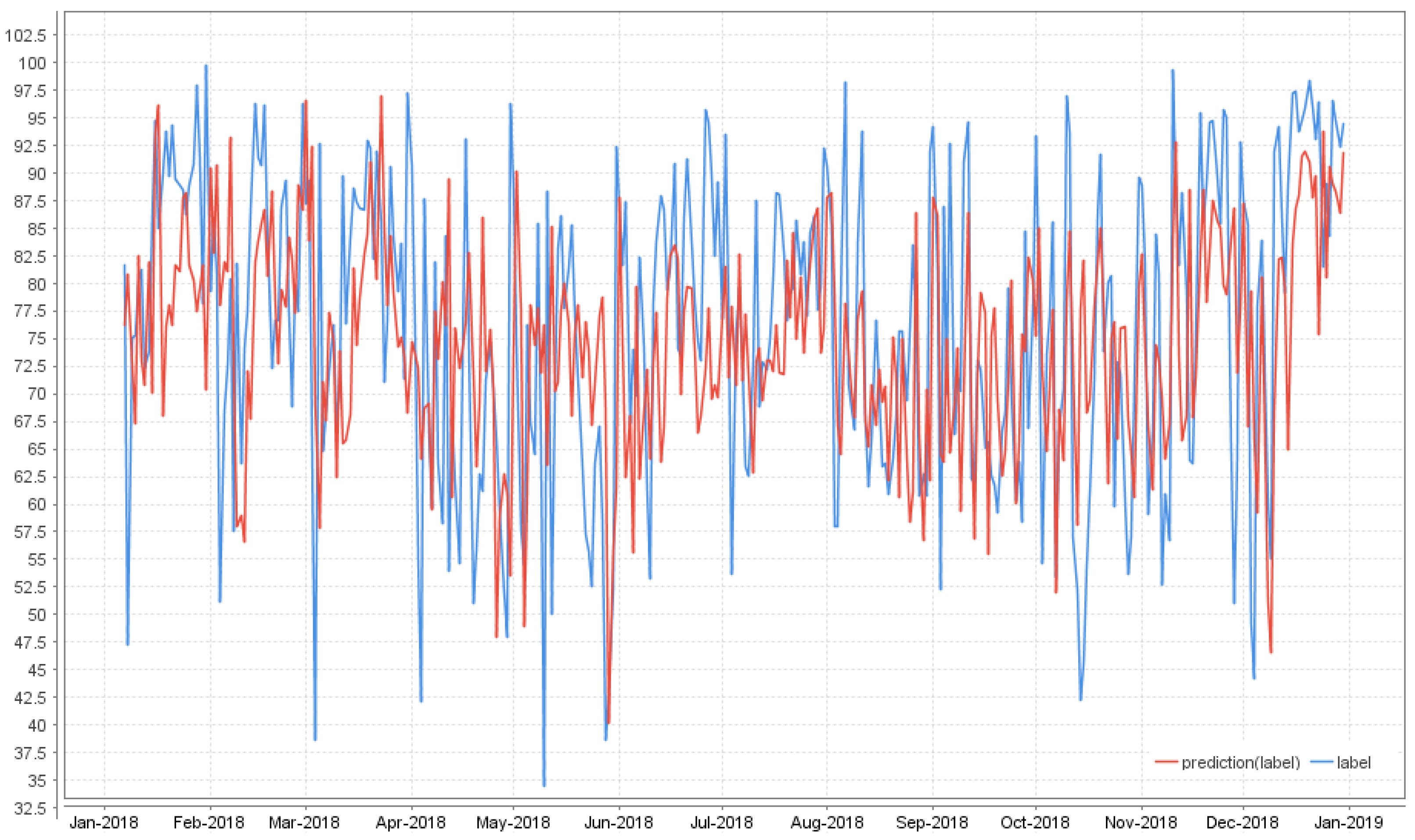
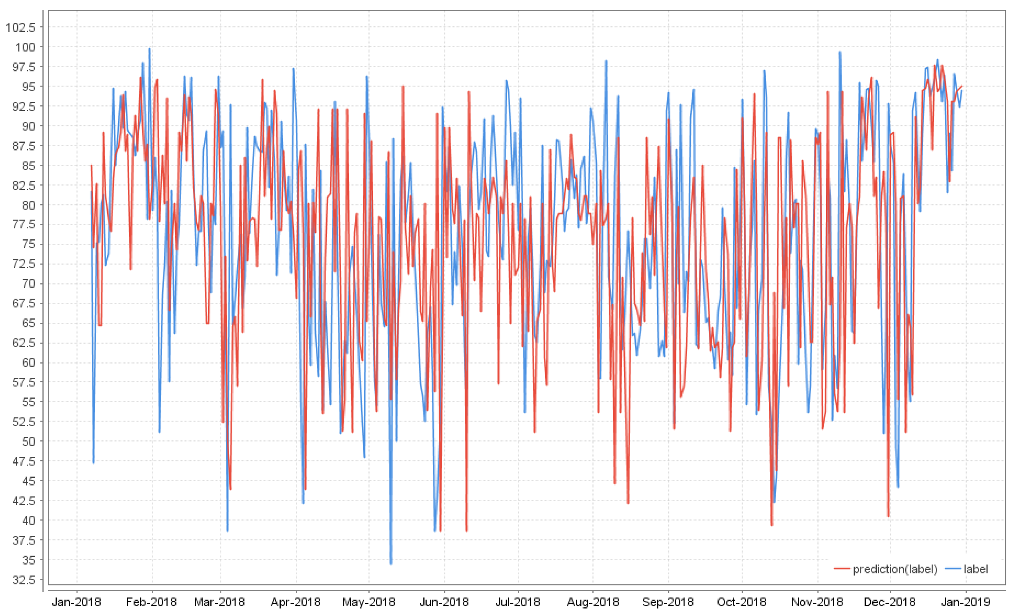
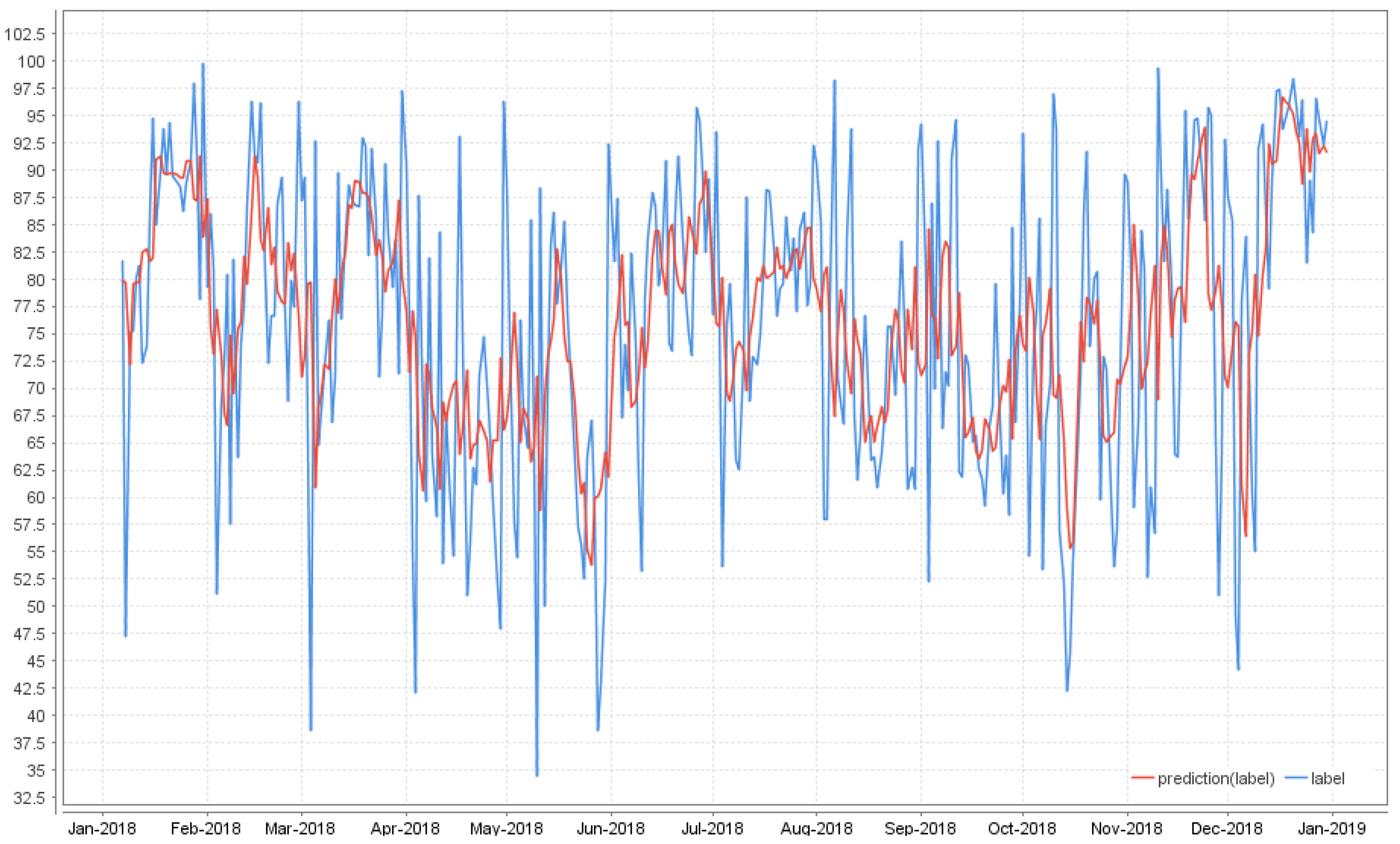
3.2. Specific Scenario Results

A deeper analysis can be performed for a specific location, for each candidate scenario and algorithm, to understand the way the prediction fluctuates versus the actual value. For example, for the test scenario CADM + CDM 3 sources, for a specific location (Sarmasu) we could check the graphical overview of the variations of the predictions for each algorithm studied. Figure 8 offers the overview for the DL algorithm, Figure 9 for the DT, while Figure 10 and Figure 11 present the overview for GBT, respectively k-NN. In blue is the graphical representation of the soil humidity value, while in red are represented the predicted values.
Figure 12 depicts the differences between actual and predicted values for all the algorithms, while Table 8 presents the standard deviation overview for the values represented.
It can be observed that the lowest deviation is produced by the GBT algorithm, but if we look at the representation, it can be concluded that the reason this happens is because the predicted value varies around the average of the actual value with the chosen setup for the algorithm, making it not a valid option in the soil moisture prediction scenario, when one would expect predictions closer to the real value. Hence, the best candidates for the problem are k-NN and DL algorithms.
As k-NN has the best performance, further we present details of the mean squared errors (MSE) (Figure 13) and the standard deviations (in Figure 14) obtained using k-NN with various setups. In Figure 13 and Figure 14, the X-axis is coded as loc_context_colsrc1_colsrc2_colsrc3, where loc is the location for which the prediction is run, context is the contextual data for that location, colsrc1, colsrc2 and colsrc3 are the collaborative data sources. When the question mark appears, it means that that data source is missing.
Figure 13 shows that the highest errors occurs when there is just one data source, respectively when there are all of them—the data from the location at stake, the context and the three collaborative data sources. In the former case, the high error is due to the relatively low amount of data available, whereas in the latter one, the error occurs from the redundant quantity of data and the possible conflicts among them (as they are not fully correlated, as expected). The best results (lowest errors) are obtained when there are two or three data sources.
An interesting point, shown in Figure 15, is that between the RMSE and the standard deviations there is a very high correlation, of 0.953, which means that a high error means more or less a high standard deviation and vice-versa.

4. Conclusions

Considering the rapid increase of available data, no matter the domain, finding improvements in the way data mining processes are performed is a subject of continuous research. Previous work has shown the advantages of using CADM and CDM techniques over the classic data mining process. The current work presents the basis of a new technique for combining the two approaches in a flexible way that allows testing the performance of different scenarios, easily configurable by the user.
The technique was then applied on a simple real life scenario for predicting the soil humidity for more locations. Once again was proven that CADM and CDM improve the classical standalone results. The algorithm with the best overall results was k-NN, followed by DL. The advantages of using the proposed technique for testing various CADM − CDM scenarios are:
  • the possibility to embed the context of the main data source;
  • the possibility to embed correlated data and apply machine learning techniques on all of them;
  • allowing to test multiple variations of scenarios in a single run, without human intervention;
  • rapid introduction of a new testing scenario, if needed;
  • flexibility in easily adding a new machine learning algorithm to be tested;
  • adding a new attribute to the context or to the correlated source is only a configuration task, not influencing the overall process.
The described technique was thought and tested in the CADM + CDM scenarios, because testing various combinations was costly and usually meant creating new processes for each scenario. By using the new approach, it changed in a configuration process. If context and collaborative sources are not present, the tested situation is the traditional data mining process.
For now, the current research focused on defining and implementing a flexible technique that would allow combining the CADM and CDM approaches in various test scenarios, to provide useful insights and support for deciding which is the best suitable approach for a specific real situation. As this part was successfully covered, the analysis of the results is yet a step that had to be performed and was based mainly on the experience of the user. Considering this, further research might improve that part by defining important criteria that would make a scenario the best one for forecasting. The process could then be improved by introducing this criteria and make a preliminary analysis of the results by performing a scoring on the performance of each test scenario. Also statistical analysis of the results could be performed.
A step further on the research would be validating the technique on larger, more complex data sets also from other domains of interest.

Author Contributions

Conceptualization, A.A., O.M. and C.A.; methodology, A.A. and C.A.; software, A.A., O.M. and C.A.; validation, A.A., O.M. and C.A.; formal analysis, A.A. and O.M.; investigation, A.A., O.M., C.P. and C.A.; resources, C.A.; data curation, A.A.; writing—original draft preparation, A.A and C.A.; writing—review and editing, A.A., O.M., and C.P.; visualization, A.A.; supervision, O.M.; project administration, O.M. and C.P.; funding acquisition, O.M. All authors have read and agreed to the published version of the manuscript.

Funding

This work has received funding from the CHIST-ERA BDSI BIG-SMART-LOG and UEFISCDI COFUND-CHIST-ERA-BIG-SMART-LOG Agreement no. 100/01.06.2019.

Conflicts of Interest

The authors declare no conflict of interest.

Abbreviations

The following abbreviations are used in this manuscript:
CADMContext-aware data mining
CDMCollaborative data mining
DLDeep Learning
DTDecision Tree
GBTGradient Boosted Tree
IoTInternet of Things
k-NNk-Nearest Neighbour
RERelative Error
RMSERoot Mean Squared error
SVMSupport Vector Machine

References

  1. Han, J.; Pei, J.; Kamber, M. Data Mining: Concepts and Techniques; Elsevier: Amsterdam, The Netherlands, 2011. [Google Scholar]
  2. Crisan, G.C.; Pintea, C.; Chira, C. Risk assessment for incoherent data. Environ. Eng. Manag. J. 2012, 11, 2169–2174. [Google Scholar] [CrossRef]
  3. Stahl, F.; Gaber, M.M.; Bramer, M.; Philip, S.Y. Pocket data mining: Towards collaborative data mining in mobile computing environments. IEEE Tools Artif. Intell. 2010, 2, 323–330. [Google Scholar]
  4. Correia, F.; Camacho, R.; Lopes, J.C. An architecture for collaborative data mining. In Proceedings of the KDIR 2010—International Conference on Knowledge Discovery and Information Retrieval, Valencia, Spain, 25–28 October 2010; SciTePress: Setubal, Portugal, 2010; pp. 467–470. [Google Scholar]
  5. Fenza, G.; Fischetti, E.; Furno, D.; Loia, V. A hybrid context aware system for tourist guidance based on collaborative filtering. In Proceedings of the IEEE International Conference on Fuzzy Systems (FUZZ-IEEE 2011), Taipei, Taiwan, 27–30 June 2011; pp. 131–138. [Google Scholar]
  6. Matei, O.; Anton, C.; Bozga, A.; Pop, P. Multi-layered architecture for soil moisture prediction in agriculture 4.0. In Proceedings of the Computers and Industrial Engineering, CIE, Lisboa, Portugal, 11–13 October 2017; Volume 2, pp. 39–48. [Google Scholar]
  7. Matei, O.; Anton, C.; Scholze, S.; Cenedese, C. Multi-layered data mining architecture in the context of Internet of Things. In Proceedings of the IEEE International Conference on Industrial Informatics, INDIN 2017, Emden, Germany, 24–26 July 2017; pp. 1193–1198. [Google Scholar]
  8. Weiser, M.; Gold, R.; Brown, J.S. The origins of ubiquitous computing research at PARC in the late 1980s. IBM Syst. J. 1999, 38, 693–696. [Google Scholar] [CrossRef]
  9. Bouquet, P.; Giunchiglia, F.; Van Harmelen, F.; Serafini, L.; Stuckenschmidt, H. C-owl: Contextualizing ontologies. In Proceedings of the 2nd International Semantic Web Conference, Sanibel Island, FL, USA, 20–23 October 2003; Springer: Berlin, Germany, 2003; pp. 164–179. [Google Scholar]
  10. Voida, S.; Mynatt, E.D.; MacIntyre, B.; Corso, G.M. Integrating virtual and physical context to support knowledge workers. IEEE Pervas. Comput. 2002, 1, 73–79. [Google Scholar] [CrossRef] [Green Version]
  11. Avram, A.; Matei, O.; Pintea, C.-M.; Pop, P.C.; Anton, C.A. Context-Aware Data Mining vs Classical Data Mining: Case Study on Predicting Soil Moisture. In Proceedings of the SOCO 2019, Advanced Computing and Systems for Security, Seville, Spain, 13–15 May 2019; Springer: Berlin, Germany, 2019; Volume 950, pp. 199–208. [Google Scholar]
  12. Anton, C.A.; Avram, A.; Petrovan, A.; Matei, O. Performance Analysis of Collaborative Data Mining vs Context Aware Data Mining in a Practical Scenario for Predicting Air Humidity. In Proceedings of the CoMeSySo 2019, Computational Methods in Systems and Software, Zlin, Czech Republic, 10–12 September 2019; Springer: Berlin, Germany, 2019; Volume 1047, pp. 31–40. [Google Scholar]
  13. Mladenic, D.; Lavrač, N.; Bohanec, M.; Moyle, S. Data Mining and Decision Support: Integration and Collaboration; Springer Science & Business Media: Berlin, Germany, 2003. [Google Scholar]
  14. Blockeel, H.; Moyle, S. Collaborative data mining needs centralised model evaluation. In Proceedings of the ICML-2002 Workshop on Data Mining Lessons Learned, Sydney, Australia, 8–12 July 2002; pp. 21–28. [Google Scholar]
  15. Anton, C.A.; Matei, O.; Avram, A. Collaborative data mining in agriculture for prediction of soil moisture and temperature. In Proceedings of the CSOC 2019, Advances in Intelligent Systems and Computing, Zlin, Czech Republic, 24–27 April 2019; Springer: Berlin, Germany, 2019; Volume 984, pp. 141–151. [Google Scholar]
  16. Matei, O.; Di Orio, G.; Jassbi, J.; Barata, J.; Cenedese, C. Collaborative data mining for intelligent home appliances. In Proceedings of the Working Conference on Virtual Enterprises, Porto, Portugal, 3–5 Ocotber 2016; Springer: Berlin, Germany, 2016; pp. 313–323. [Google Scholar]
  17. Dey, A.K. Understanding and using context. Pers. Ubiquit. Comput. 2001, 5, 4–7. [Google Scholar] [CrossRef]
  18. Lee, S.; Chang, J.; Lee, S.G. Survey and trend analysis of context-aware systems. Information 2011, 14, 527–548. [Google Scholar]
  19. Yang, S.J. Context aware ubiquitous learning environments for peer-to-peer collaborative learning. J. Educ. Tech. Soc. 2006, 9, 188–201. [Google Scholar]
  20. Stokic, D.; Scholze, S.; Kotte, O. Generic self-learning context sensitive solution for adaptive manufacturing and decision making systems. In Proceedings of the ICONS14 International Conference on Systems, Nice, France, 23–27 February 2014; pp. 23–27. [Google Scholar]
  21. Scholze, S.; Barata, J.; Stokic, D. Holistic context-sensitivity for run-time optimization of flexible manufacturing systems. Sensors 2017, 17, 455. [Google Scholar] [CrossRef] [Green Version]
  22. Perera, C.; Zaslavsky, A.; Christen, P.; Georgakopoulos, D. Context aware computing for the internet of things: A survey. IEEE Commun. Surv. Tut. 2013, 16, 414–454. [Google Scholar] [CrossRef] [Green Version]
  23. Scholze, S.; Kotte, O.; Stokic, D.; Grama, C. Context-sensitive decision support for improved sustainability of product lifecycle. In Proceedings of the Intelligent Decision Technologies, KES-IDT, Sesimbra, Portugal, 26–28 June 2013; Volume 255, pp. 140–149. [Google Scholar]
  24. Vajirkar, P.; Singh, S.; Lee, Y. Context-aware data mining framework for wireless medical application. In Proceedings of the International Conference on Database and Expert Systems Applications DEXA, Prague, Czech Republic, 1–5 September 2003; Springer: Berlin, Germany, 2003; Volume 2736, pp. 381–391. [Google Scholar]
  25. Marakas, G.M. Modern Data Warehousing, Mining, and Visualization: Core Concepts; Prentice Hall: Upper Saddle River, NJ, USA, 2003. [Google Scholar]
  26. Ziafat, H.; Shakeri, M. Using data mining techniques in customer segmentation. J. Eng. Res. App. 2014, 4, 70–79. [Google Scholar]
  27. Vashenyuk, E.; Balabin, Y.; Germanenko, A.; Gvozdevsky, B. Study of radiation related with atmospheric precipitations. Proc. ICRC Beijing 2011, 11, 360–363. [Google Scholar]
  28. Sitnov, S.; Mokhov, I.; Gorchakov, G. The link between smoke blanketing of European Russia in summer 2016, Siberian wildfires and anomalies of large-scale atmospheric circulation. In Doklady Earth Sciences; Springer: Berlin, Germany, 2017; Volume 472, pp. 190–195. [Google Scholar]
  29. Weather Prognosis. Available online: https://rp5.ru/ (accessed on 1 April 2020).
  30. Current and Historical Alberta Weather Station Data Viewer. Available online: http://agriculture.alberta.ca/acis/weather-data-viewer.jsp (accessed on 1 April 2020).
  31. Land, S.; Fischer, S. Rapid Miner 5. RapidMiner in Academic Use; Rapid-I GmbH: Dortmund, Germany, 2012. [Google Scholar]
  32. Hofmann, M.; Klinkenberg, R. RapidMiner: Data Mining Use Cases and Business Analytics Applications; CRC Press: Boca Raton, FL, USA, 2016. [Google Scholar]
  33. Kumar, R.; Balara, A. Time series forecasting of nifty stock market using Weka. Int. J. Res. Publ. Sem. 2014, 5, 1–6. [Google Scholar]
  34. Li, Y.; Yang, P.; Wang, H. Short-term wind speed forecasting based on improved ant colony algorithm for LSSVM. Cluster Comput. 2019, 22, 11575–11581. [Google Scholar] [CrossRef]
  35. Pintea, C.M.; Crisan, G.C.; Chira, C. Hybrid ant models with a transition policy for solving a complex problem. Logic J. IGPL 2011, 20, 560–569. [Google Scholar] [CrossRef]
  36. Nayak, J.; Vakula, K.; Dinesh, P.; Naik, B.; Mishra, M. Ant Colony Optimization in Data Mining: Critical Perspective from 2015 to 2020. In Innovation in Electrical Power Engineering, Communication, and Computing Technology; Springer: Belrin, Germany, 2020; pp. 361–374. [Google Scholar]
  37. Azzag, H.; Guinot, C.; Venturini, G. Data and text mining with hierarchical clustering ants. Stud. Comput. Intell. 2006, 34, 153–189. [Google Scholar]
  38. Koskela, T.; Varsta, M.; Heikkonen, J.; Kaski, K. Time series prediction using recurrent SOM with local linear models. Int. J. Knowl. Based Intell. Eng. Syst. 1998, 2, 60–68. [Google Scholar]
  39. Cunningham, P.; Delany, S.J. k-Nearest neighbour classifiers. Mult. Classif. Syst. 2007, 34, 1–17. [Google Scholar]
  40. Fawaz, H.I.; Forestier, G.; Weber, J.; Idoumghar, L.; Muller, P.A. Deep learning for time series classification: A review. Data Min. Knowl. Disc. 2019, 33, 917–963. [Google Scholar] [CrossRef] [Green Version]
  41. Yu, C.; Li, Y.; Xiang, H.; Zhang, M. Data mining-assisted short-term wind speed forecasting by wavelet packet decomposition and Elman neural network. J. Wind Eng. Ind. Aerod. 2018, 175, 136–143. [Google Scholar] [CrossRef]
  42. Geurts, P. Contributions to Decision Tree Induction: Bias/variance Tradeoff and Time Series Classification. Ph.D. Thesis, University of Liège, Liège, Belgium, 2002. [Google Scholar]
  43. Hyndman, R.J.; Athanasopoulos, G. Forecasting: Principles and Practice; OTexts: Melbourne, Australia, 2014. [Google Scholar]
  44. Abramowitz, M.; Stegun, I.A. Handbook of Mathematical Functions: With Formulas, Graphs, and Mathematical Tables; Dover Publications: Mineola, NY, USA, 1965. [Google Scholar]
  45. Hyndman, R.J.; Koehler, A.B. Another look at measures of forecast accuracy. Int. J. Forecast. 2006, 22, 679–688. [Google Scholar] [CrossRef] [Green Version]
  46. Dodge, Y. Spearman Rank Correlation Coefficient. The Concise Encyclopedia of Statistics; Springer: New York, NY, USA, 2008; pp. 502–505. [Google Scholar]
  47. Schmid, F.; Schmidt, R. Multivariate extensions of Spearman’s rho and related statistics. Stat. Probab. Lett. 2007, 77, 407–416. [Google Scholar] [CrossRef]
Figure 1. Innovation: Context-Aware Data Mining (CADM) and Collaborative Data Mining (CDM) combined process overview, influenced by Reference [12].
Mathematics 08 00684 g001
Figure 2. Scenarios Platform-Collaborative & Context-Aware Data Mining (SP-CCADM) flow chart.
Mathematics 08 00684 g002
Figure 3. Relative Error (RE) representation for the initial testing phase during various time windows (from 1 to 30 days): time windows (X-axis) and the obtained RE values (Y-axis).
Mathematics 08 00684 g003
Figure 4. Relative Error (RE) representation for k-Nearest Neighbors (k-NN) during the optimization parameter process: values tested for k (X-axis) and the obtained RE values (Y-axis).
Mathematics 08 00684 g004
Figure 5. Relative Error (RE) representation for Decision Trees (DT) during the optimization parameters process: the values tested for DT maximal depth (X-axis) and the RE obtained values (Y-axis).
Mathematics 08 00684 g005
Figure 6. Relative Error (RE) representation of the overall results grouped by the tested algorithm: the algorithms (X-axis) and the RE obtained values (Y-axis).
Mathematics 08 00684 g006
Figure 7. Relative Error (RE) overview representation per location and algorithm: location and algorithm tested (X-axis) and the RE obtained values (Y-axis).
Mathematics 08 00684 g007
Figure 8. Deep Learning (DL) prediction overview for Sarmasu: CADM + CDM 3 sources scenario: the values for the actual value, in blue, and predicted value, in red (X-axis) and the time series for which the results were registered (Y-axis).
Mathematics 08 00684 g008
Figure 9. Decision Tree (DT) prediction overview for Sarmasu: CADM + CDM 3 sources scenario: the values for the actual value, in blue, and predicted value, in red (X-axis) and the time series for which the results were registered (Y-axis).
Mathematics 08 00684 g009
Figure 10. Gradient Boosted Tree (GBT) prediction overview for Sarmasu: CADM + CDM 3 sources scenario: the values for the actual value, in blue, and predicted value, in red (X-axis) and the time series for which the results were registered (Y-axis).
Mathematics 08 00684 g010
Figure 11. k-Nearest Neighbor (k-NN) prediction overview for Sarmasu: CADM + CDM 3 sources scenario: the values for the actual value, in blue, and predicted value, in red (X-axis) and the time series for which the results were registered (Y-axis).
Mathematics 08 00684 g011
Figure 12. Prediction variation overview for Sarmasu: CADM + CDM 3 sources scenario for DT & k-NN (upper side) and GBT & DL (lower side) the values for the deviation of predicted value versus actual value (X-axis) and the time series for which the results were registered (Y-axis).
Mathematics 08 00684 g012
Figure 13. The RMSEs for k-NN algorithm with various setups: loc_context_colsrc1_colsrc2_colsrc3 (X-axis) where loc is the location for which the prediction is run, context is the contextual data for that location, colsrc1, colsrc2 and colsrc3 are the collaborative data sources, and the value of RMSE (Y-axis); ? denotes missing data source.
Mathematics 08 00684 g013
Figure 14. The standard deviations for k-NN algorithm with various setups: loc_context_colsrc1_colsrc2_colsrc3 (X-axis) where loc is the location for which the prediction is run, context is the contextual data for that location, colsrc1, colsrc2 and colsrc3 are the collaborative data sources, and the value of standard deviation (Y-axis); ? denotes missing data source.
Mathematics 08 00684 g014
Figure 15. The correlation between RMSE and the standard deviation: the RMSE (X-axis) and the standard deviation (Y-axis).
Mathematics 08 00684 g015
Table 1. Scenarios Platform-Collaborative & Context-Aware Data Mining (SP-CCADM) example: a hybrid CADM-CDM test scenarios to be covered in the analysis, where ? are ignored attributes.
Main DataContext AttributesCollaborative Sources
C S 1 C S P
A M 1 A MP A M n A C 1 A C k A CS 1 A CS 1 A CS 1 A CS j
val val valval valval val val val
val val valval valval val ? ?
val val valval val? ? ? ?
val val val? ?val val val val
val val val? ?? ? val val
val val val? ?? ? ? ?
Table 2. Overview of Data Sources with details about considered Time interval (time series), the name of locations from Data Sources and where to find data on public websites.
Data SourcesTime IntervalLocationsPublic Data
6 locations in Transylvania,
Romania
01.01.2016 to 31.12.2018Sarmasu, Reghin, Targu Mures,
Ludus, Blaj, Dumbraveni
website [29]
4 locations in Alberta Province,
Canada
01.05.2018 to 01.04.2020Breton, St. Albert,
Tomahawk, Leedale
website [30]
Table 3. The correlation matrix of the data sources from the six locations [29].
CampeniSarmasuTMuresReghinLudusBlajDumbraveni
Campeni10.7510.7430.6510.7290.7850.741
Sarmasu0.75110.9020.8800.9310.8670.858
TMures0.7430.90210.8610.8690.8860.920
Reghin0.6510.8800.86110.8860.9830.845
Ludus0.7290.9930.8670.99610.7840.845
Blaj0.7850.8670.8860.9830.78410.896
Dumbraveni0.7410.8580.9200.8450.8450.8961
Table 4. Relative Error (RE) results for Deep Learning (DL) in the parameter optimization process.
Activation: TanhActivation: RectifierActivation: ExpRectifier
EpochsREEpochsREEpochsRE
20.16357267520.13594280520.145482752
40.15802291840.14678032640.175774121
60.15739831560.18266082960.172397822
80.17456071180.19200592880.184494165
100.159373990100.121232879100.136397852
150.175305445150.186658629150.173097985
Table 5. Machine learning algorithms parameters setting.
k-NNGBTDTDL
k:5Number of Trees:50Maximal depth:4Activation:Rectifier
Measure:EuclideanMaximal depth:7Minimal gain:0.01Epochs:5
distanceLearning rate:0.01Minimal leaf size:2
Number of bins:20
Table 6. Example of combined test scenarios used in the experiments. Notations: H_Location and T_Location denotes the humidity (H) and respectively the temperature (T) of the specified location.
PredictedContextCorrelated
Source 1
Correlated
Source 2
Correlated
Source 3
Scenario
H_SarmasuT_SarmasuH_ReghinH_TMuresH_LudusCADM+CDM 3 sources
H_SarmasuT_SarmasuH_ReghinH_TMures?CAD+CDM 2 sources
H_SarmasuT_SarmasuH_Reghin??CADM+CDM 1 source
H_SarmasuT_Sarmasu???CADM
H_Sarmasu?H_ReghinH_TMuresH_LudusCDM 3 sources
H_Sarmasu????Standalone
H_TMuresT_TMuresH_ReghinH_SarmasuH_LudusCADM+CDM 3 sources
H_TMuresT_TMuresH_ReghinH_Sarmasu?CADM+CDM 2 sources
H_TMuresT_TMuresH_Reghin??CADM+CDM 1 source
H_TMuresT_TMures???CADM
H_TMures?H_ReghinH_SarmasuH_LudusCDM 3 sources
H_TMures????Standalone
Table 7. Spearman ρ overall results for Data Sources [29,30] described in Table 2 and tested scenarios.
Data SourceScenarioDLDTGBTkNN
TransylvaniaCADM0.809820.742040.870510.81566
TransylvaniaCADM + CDM 1 source0.845930.737650.881720.82123
TransylvaniaCADM + CDM 2 sources0.859320.755000.891840.81689
TransylvaniaCADM + CDM 3 sources0.863580.762170.871030.83141
TransylvaniaStandalone0.826570.722640.874480.81372
TransylvaniaCDM + 3 sources0.837300.760770.876310.81345
CanadaCADM0.615480.834490.876270.87236
CanadaCADM + CDM 1 source0.731430.834470.876270.87513
CanadaCADM + CDM 2 sources0.662000.834500.874120.87429
CanadaCADM + CDM 3 sources0.702110.895230.865050.90480
CanadaStandalone0.720110.802760.874120.86220
CanadaCDM + 3 sources0.662650.834500.898180.88124
Table 8. Standard deviation overview per algorithm for Sarmasu in the CADM + CDM 3 sources scenario.
AlgValueStandard DeviationStandard Deviation(%)
k-NN0.1383815770.02639699119.08
DL0.1483579620.0270554418.24
GBT0.1474885670.01978161313.41
DT0.1505156140.03372887422.41

