Rational Transformations for Evaluating Singular Integrals by the Gauss Quadrature Rule

Abstract

In this work we introduce new rational transformations which are available for numerical evaluation of weakly singular integrals and Cauchy principal value integrals. The proposed rational transformations include parameters playing an important role in accelerating the accuracy of the Gauss quadrature rule used for the singular integrals. Results of some selected numerical examples show the efficiency of the proposed transformation method compared with some existing transformation methods.

1. Introduction

We consider numerical evaluation of weakly singular integrals and Cauchy principal value(CPV) integrals which frequently appear, for instance, in the dominant coefficients of the boundary element method [1,2,3,4,5]. Accurate evaluation of these singular integrals is a very practical and important problem in many areas of engineering including elastostatics and electromagnetics.

Until now, lots of numerical methods for evaluation of the singular integrals have been developed. Among the methods one can notice that the nonlinear coordinate transformation techniques [6,7,8,9,10,11,12,13,14,15,16,17,18] are prominent as they are easy to use in adaptive approaches. Thus, aiming enhancement of the accuracy of the numerical integration method via the coordinate transformation, in this paper we present simple rational functions including parameters. Then we explore the availability of the proposed rational transformation method for each type of singular integrals.

In the following section we define rational functions $f_m(\eta ;t)$ in (11) for weakly singular integrals with an interior-point singularity and ${\tilde{f}}_m(k;t)$ in (15) for those with an end-point singularity. The proposed rational functions, satisfying some appropriate properties, weaken the singularity of the integrand. These rational functions associated with a standard quadrature rule are expected to improve approximation errors further by controlling the parameters $\eta$ and k.

In Section 3, for the CPV integrals we suggest a composite function $F_m(\eta ;t)$ in (40) which is composed of the rational function $f_m(\eta ;t)$ and a quadratic function $g(\eta ;t)$ in (31). The coordinate transformation using $F_m(\eta ;t)$ has an important property which vanishes the singular part of the CPV integral when any even number of integration points are used. Thus, like the case of the weakly singular integrals, we may efficiently evaluate CPV integrals by employing the composite function $F_m(\eta ;t)$ with $\eta$ selected in a proper range.

For numerical experiments we choose some examples of the singular integrals at the end of each section. Numerical results of the presented method associated with the Gauss-Legendre quadrature rule show the competent errors for the end-point weakly singular integrals. Moreover, for the CPV integral the presented transformation method with the parameter $\eta$ selected within an appropriate region results in much better errors than the existing transformation methods.

2. Weakly Singular Integrals

For a point $-1\le x_0\le 1$, we consider the weakly singular integrals

$$\begin{array}{c}\hfill I_{\alpha }\varphi \left(x_0\right):={\int }_{-1}^1{|x-x_0|}^{\alpha }\varphi \left(x\right)dx,-1<\alpha <0\end{array}$$

(1)

and

$$\begin{array}{c}\hfill J\varphi \left(x_0\right):={\int }_{-1}^1\varphi \left(x\right)log|x-x_0|dx.\end{array}$$

(2)

We set $s_0=x_0$ when $|x_0|<1$ and ${\xi }_0=x_0$ when $|x_0|=1$ throughout this work.

2.1. Existing Transformations

For a weakly singular integral with an interior-point singularity at $s_0$ with $\left|s_0\right|<1$ there are useful nonlinear transformations which do not require any division of the integration interval as follows.

•

Telles polynomial transformation [15]:

$$P_3^{\mathrm{Tel}}\left(t\right)=\frac{1}{1+3{\gamma }^2}\left(3\gamma +3{\gamma }^{2}t-3\gamma t^2+t^3\right),-1\le t\le 1,$$

(3)

where $\gamma =(s_0{s}^{*}+|s^{*}{\left|\right)}^{1/3}+(s_0{\xi }^{*}-|s^{*}{\left|\right)}^{1/3}+s_0$ with $s^{*}=s_0^2-1$.

•

Monegato–Sloan polynomial transformation [19]:

$$P_m^{\mathrm{MS}}\left(t\right)=s_0+\delta \left(s_0,m\right){\left(t-{\eta }_0\right)}^m,-1\le t\le 1,$$

(4)

where

$$\delta \left(s_0,m\right)=2^{-m}{\left\{{\left(1+s_0\right)}^{1/m}+{\left(1-s_0\right)}^{1/m}\right\}}^m,$$

${\eta }_0$ is a point defined by

$${\eta }_0=\frac{{\left(1+s_0\right)}^{1/m}-{\left(1-s_0\right)}^{1/m}}{{\left(1+s_0\right)}^{1/m}+{\left(1-s_0\right)}^{1/m}}$$

and $m\ge 1$ is an odd integer.

•

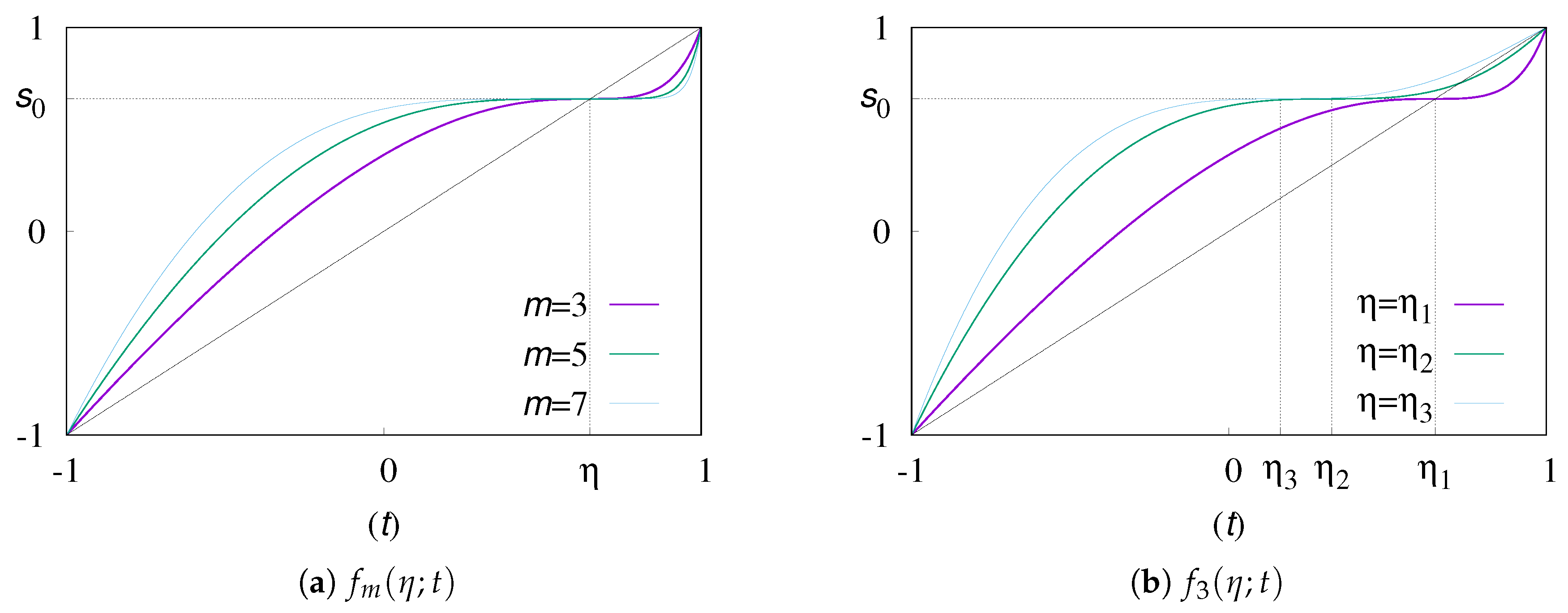
Generalized sigmoidal transformation [16]:

$${\mathsf{\Psi }}_m\left(t\right)=s_0+2\mathrm{Sgn}(t-{\eta }_0){\gamma }_m\left(\frac{|t-{\eta }_0|}{2}\right),-1\le t\le 1,$$

(5)

where ${\gamma }_m\left(\tau \right)$, $0\le \tau \le 1$, is a sigmoidal transformation of order m(see [8,9] for the definition) with the behavior $O\left({\tau }^m\right)$ near $\tau =0$, ${\eta }_0$ is a point transformed as

$${\eta }_0=2{\gamma }_m^{-1}\left(\frac{1+s_0}{2}\right)-1$$

(6)

and $\mathrm{Sgn}\left(t\right)$ is the sign function whose value is 1 for $t>0$ and $-1$ for $t<0$.

It is noted that both $P_m^{\mathrm{MS}}$ and ${\mathsf{\Psi }}_m$ have the following asymptotic behavior near the transformed singular point $t={\eta }_0$.

$$s_0+O\left({\left(t-{\eta }_0\right)}^m\right).$$

(7)

Thus, by the change of variable $x=P_m^{\mathrm{MS}}\left(t\right)$ or $x={\mathsf{\Psi }}_m\left(t\right)$ in Equations (1) and (2), the weakly singular integrals $I_{\alpha }\varphi$ and $J\varphi$ become regular ones for m large enough because the behaviors of the integrands are transformed to $O\left({\left(t-{\eta }_0\right)}^{(\alpha +1)m-1}\right)$ and $O\left({\left(t-{\eta }_0\right)}^{m-1}log\left|t-{\eta }_0\right|\right)$, respectively, near $t={\eta }_0$.

For a weakly singular integral with an end-point singularity at ${\xi }_0$ with $\left|{\xi }_0\right|=1$ we introduce two famous transformations below.

•

Sato polynomial transformation [14]:

$$P_m^{\mathrm{Sat}}\left(t\right)={\xi }_0\left\{1-\frac{{(1-{\xi }_{0}t)}^m}{2^{m-1}}\right\},-1\le t\le 1,$$

(8)

where m is an integer $m\ge 2$.

•

Semi-sigmoidal transformation [10]:

$${\tilde{\gamma }}_m\left(t\right)={\xi }_0\left\{1-4{\gamma }_m\left(\frac{1-{\xi }_{0}t}{4}\right)\right\},-1\le t\le 1.$$

(9)

Both $P_m^{\mathrm{Sat}}$ and ${\tilde{\gamma }}_m$ have the following asymptotic behavior near $t={\xi }_0$.

$${\xi }_0+O\left({\left(t-{\xi }_0\right)}^m\right).$$

(10)

2.2. A Rational Transformation

For an interior-point singularity at $s_0$ with $\left|s_0\right|<1$ we define a rational transformation

$$f_m(\eta ;t)=s_0+\left(1-s_{0}t\right){\left\{\frac{t-\eta }{1-\eta t}\right\}}^m,-1\le t\le 1,$$

(11)

where $m\ge 1$ is an odd integer and $\eta$ is a real number such that $\left|\eta \right|<1$. It has the features

$$f_m(\eta ;-1)=-1,f_m(\eta ;\eta )=s_0,f_m(\eta ;1)=1$$

(12)

independently of $\eta$ and

$$\frac{d{f}_m}{dt}(\eta ;t)=\frac{m(1-s_{0}t)(1-{\eta }^2)+s_0(\eta t-1)(t-\eta )}{{(1-\eta t)}^2}{\left\{\frac{t-\eta }{1-\eta t}\right\}}^{m-1}.$$

(13)

For simplicity we assume that $0\le s_0<1$. Then, for any $\eta$ such that

$$\eta \ge -1+\frac{2s_0}{m(1-s_0)+s_0}$$

(14)

with m fixed, we can see that $\frac{d{f}_m}{dt}(\eta ;t)\ge 0$ for all $-1<t<1$ so that $f_m$ is bijective on the interval $[-1,1]$. See Figure 1 for the insight of the function $f_m$ with $s_0=0.65$. We note that for the case of $m=3$ (in Figure 1b) the condition (14) becomes $\eta \ge -\frac{4}{17}$. Setting $x=f_m(\eta ;t)$ in (1) and (2), we have the bettered integrands whose behaviors are respectively $O\left({(t-\eta )}^{(\alpha +1)m-1}\right)$ and $O({(t-\eta )}^{m-1}log|t-\eta |)$ near $t=\eta$.

For an end-point singularity at ${\xi }_0$ with $\left|{\xi }_0\right|=1$ we suggest another rational transformation ${\tilde{f}}_m$ as

$${\tilde{f}}_m(k;t)={\xi }_0+{\left(\frac{k-1}{2}\right)}^m\left(1-{\xi }_{0}t\right){\left\{\frac{t-{\xi }_0}{k+{\xi }_{0}t}\right\}}^m,-1\le t\le 1,$$

(15)

where m is an odd integer and k is a real number such that $k>1$. It satisfies

$${\tilde{f}}_m\left(k;{\xi }_0\right)={\xi }_0,{\tilde{f}}_m\left(k;-{\xi }_0\right)=-{\xi }_0$$

(16)

independently of k and

$$\frac{d{\tilde{f}}_m}{dt}(k;t)=\frac{2^{-m}{(1-k)}^m\left(m{\xi }_0+k(m+1){\xi }_0+t\right)}{k+{\xi }_{0}t}{\left\{\frac{t-{\xi }_0}{k+{\xi }_{0}t}\right\}}^m>0$$

(17)

for all $-1<t<1$, which implies that ${\tilde{f}}_m$ is bijective on the interval $[-1,1]$. In addition, near the end pint ${\xi }_0$ the function ${\tilde{f}}_m$ has the asymptotic behavior

$${\tilde{f}}_m\left(k;t\right)={\xi }_0-{\xi }_0{\left(\frac{k-1}{2(k+1)}\right)}^m{\left(t-{\xi }_0\right)}^{m+1}+O\left({\left(t-{\xi }_0\right)}^{m+2}\right).$$

(18)

Figure 2 shows the graph of $\widetilde{f_3}(k;t)$, ${\xi }_0=1$, comparing it with those of $P_3^{\mathrm{Sat}}\left(t\right)$ and ${\tilde{\gamma }}_3\left(t\right)$. The graph of $\widetilde{f_3}(k;t)$ with k large enough looks similar to that of the semi-sigmoidal transformation ${\tilde{\gamma }}_3\left(t\right)$. By the change of variable $x={\tilde{f}}_m\left(k;t\right)$, the weakly singular integrals $I_{\alpha }\varphi$ and $J\varphi$ are respectively transformed to $I_{\alpha }^{\left[m\right]}\varphi$ and $J^{\left[m\right]}\varphi$ defined by

$$I_{\alpha }^{\left[m\right]}\varphi \left({\xi }_0\right)={\int }_{-1}^1{\left|{\tilde{f}}_m\left(k;t\right)-{\xi }_0\right|}^{\alpha }\varphi \left({\tilde{f}}_m\left(k;t\right)\right)\frac{d}{dt}{\tilde{f}}_m\left(k;t\right)dt$$

(19)

and

$$J^{\left[m\right]}\varphi \left({\xi }_0\right)={\int }_{-1}^1\varphi \left({\tilde{f}}_m\left(k;t\right)\right)log\left|{\tilde{f}}_m\left(k;t\right)-{\xi }_0\right|\frac{d}{dt}{\tilde{f}}_m\left(k;t\right)dt.$$

(20)

We can see that the regularity of the original integrands in (1) and (2) becomes higher as the order m of the transformation is increasing. Referring to the literature [11], we may have the asymptotic truncation errors of the N-point Gauss-Legendre quadrature rules $I_{\alpha ,N}^{\left[m\right]}\varphi$ and $J_N^{\left[m\right]}\varphi$ for the transformed integrals in (19) and (20), respectively, as follows.

$$\begin{array}{cc}\hfill E_{\alpha ,N}^{\left[m\right]}\varphi \left({\xi }_0\right)& :=I_{\alpha }^{\left[m\right]}\varphi \left({\xi }_0\right)-I_{\alpha ,N}^{\left[m\right]}\varphi \left({\xi }_0\right)\hfill \\ & \sim {C_m\left(k\right)}^{1+\alpha }·\frac{2^{2-(2m+1)(1+\alpha )}(m+1)\varphi \left({\xi }_0\right)\mathsf{\Gamma }\left(2(m+1)(1+\alpha )\right)sin\left((m+1)\alpha \pi \right)}{2^m{(2N+1)}^{2(m+1)(1+\alpha )}}\hfill \end{array}$$

(21)

and

$$\begin{array}{cc}\hfill E_N^{\left[m\right]}\varphi \left({\xi }_0\right)& :=J^{\left[m\right]}\varphi \left({\xi }_0\right)-J_N^{\left[m\right]}\varphi \left({\xi }_0\right)\hfill \\ & \sim C_m\left(k\right)·\frac{2^{2-(2m+1)}{(m+1)}^2\varphi \left({\xi }_0\right)\mathsf{\Gamma }\left(2(m+1)\right)\pi }{2^m{(2N+1)}^{2(m+1)}}\hfill \end{array}$$

(22)

for sufficiently large N. Therein, $C_m\left(k\right)$ is the leading coefficient of the asymptotic behavior of ${\tilde{f}}_m\left(k;t\right)-{\xi }_0$ near the point $t={\xi }_0$, i.e., $C_m\left(k\right)={\xi }_0{\left(\frac{k-1}{2(k+1)}\right)}^m$.

2.3. Numerical Examples

We have used the high-level computing software, Mathematica (V.11) in numerical implementation for the examples below.

Example 1.

Interior-point weakly singular integrals $I_{\alpha }\varphi \left(s_0\right)$ with $\varphi \left(x\right)\equiv 1$:

Exact value of the integral is

$$I_{\alpha }\varphi \left(s_0\right)=\frac{1}{1+\alpha }\left\{{\left(1+s_0\right)}^{1+\alpha }+{\left(1-s_0\right)}^{1+\alpha }\right\}.$$

In the numerical implementation using the proposed transformation $f_m(\eta ;t)$ we may choose the parameter $\eta$, for example, by the formula

$$\eta =\frac{2s_0}{m(1-s_0)+s_0}-s_0$$

(23)

which satisfies the inequality (14). Numerical results of the relative errors of the N-point Gauss-Legendre quadrature rule for the transformed integrand via the change of variable $x=f_m(\eta ;t)$ are given in

Table 1. Relative errors of the N-point Gauss-Legendre quadrature rule corresponding to the existing transformations $P_m^{\mathrm{MS}}\left(t\right)$, ${\mathsf{\Psi }}_m\left(t\right)$ and the presented transformation $f_m(\eta ;t)$ for the interior-point weakly singular integral $I_{\alpha }\varphi \left(s_0\right)$, with $\alpha =-0.5$ and $s_0=0.1$, in Example 1.

		Existing Transformations			Presented Transformation ${\mathit{f}}_{\mathit{m}}(\mathit{\eta };\mathit{t})$
$\mathit{m}$	$\mathit{N}$	${\mathbf{P}}_{\mathit{m}}^{\mathrm{MS}}\left(\mathit{t}\right)$	${\mathsf{\Psi }}_{\mathit{m}}\left(\mathit{t}\right)$		$\mathit{\eta }={\mathit{\eta }}_{\mathbf{1}}$	$\mathit{\eta }={\mathit{\eta }}_{\mathbf{2}}$
7	10	$3.6\times {10}^{-4}$	$3.7\times {10}^{-4}$		$\mathbf{6.4}\times {\mathbf{10}}^{-\mathbf{5}}$	$3.4\times {10}^{-4}$
	20	$3.0\times {10}^{-5}$	$\mathbf{4.4}\times {\mathbf{10}}^{-\mathbf{6}}$		$3.9\times {10}^{-5}$	$2.6\times {10}^{-5}$
	30	$6.0\times {10}^{-6}$	$\mathbf{8.4}\times {\mathbf{10}}^{-\mathbf{7}}$		$3.9\times {10}^{-6}$	$3.7\times {10}^{-6}$
	40	$1.5\times {10}^{-6}$	$2.1\times {10}^{-7}$		$2.6\times {10}^{-6}$	$\mathbf{1.2}\times {\mathbf{10}}^{-\mathbf{7}}$
11	10	$2.3\times {10}^{-5}$	$3.9\times {10}^{-3}$		$\mathbf{4.5}\times {\mathbf{10}}^{-\mathbf{6}}$	$2.2\times {10}^{-5}$
	20	$5.2\times {10}^{-7}$	$7.6\times {10}^{-7}$		$5.8\times {10}^{-7}$	$\mathbf{3.8}\times {\mathbf{10}}^{-\mathbf{7}}$
	30	$5.2\times {10}^{-8}$	$\mathbf{3.6}\times {\mathbf{10}}^{-\mathbf{9}}$		$1.4\times {10}^{-8}$	$2.2\times {10}^{-8}$
	40	$9.6\times {10}^{-9}$	$\mathbf{3.6}\times {\mathbf{10}}^{-\mathbf{10}}$		$1.3\times {10}^{-8}$	$3.7\times {10}^{-10}$
15	10	$3.0\times {10}^{-6}$	$9.6\times {10}^{-3}$		$\mathbf{1.2}\times {\mathbf{10}}^{-\mathbf{6}}$	$2.7\times {10}^{-6}$
	20	$1.6\times {10}^{-8}$	$2.4\times {10}^{-5}$		$1.6\times {10}^{-8}$	$\mathbf{1.1}\times {\mathbf{10}}^{-\mathbf{8}}$
	30	$7.6\times {10}^{-10}$	$4.7\times {10}^{-8}$		$4.5\times {10}^{-10}$	$\mathbf{2.9}\times {\mathbf{10}}^{-\mathbf{10}}$
	40	$8.4\times {10}^{-11}$	$7.9\times {10}^{-11}$		$7.9\times {10}^{-11}$	$\mathbf{4.6}\times {\mathbf{10}}^{-\mathbf{12}}$

when $\alpha =-0.5$ and $s_0=0.1$. Therein, ${\eta }_1$ is the value given by Equation (23) and ${\eta }_2=s_0/5$ which also satisfies the condition (14) for the selected singular point $s_0=0.1$. The relative error is defined as

$$\left|\frac{\mathrm{Exact}\mathrm{value}-\mathrm{Approximate}\mathrm{value}}{\mathrm{Exact}\mathrm{value}}\right|.$$

(24)

For comparison with the existing transformation methods, Table 1 also includes numerical results corresponding to the Monegato–Sloan polynomial transformation $P_m^{\mathrm{MS}}\left(t\right)$ in (4) and the generalized sigmoidal transformation ${\mathsf{\Psi }}_m\left(t\right)$ in (5). The best errors are indicated by the bold numbers. We can see that the results of the proposed rational transformation seem to be comparable to those of the existing ones. For any $-1<s_0<1$ we have the similar tendency of the numerical results to those given in Table 1.

Example 2.

End-point weakly singular integrals $I_{\alpha }\varphi \left({\xi }_0\right)$ with $\varphi \left(x\right)\equiv 1$ and $J\varphi \left({\xi }_0\right)$ with $\varphi \left(x\right)=1+x^2$:

Exact value of the integrals are

$$I_{\alpha }\varphi \left({\xi }_0\right)=\frac{2^{1+\alpha }}{1+\alpha }$$

and

$$J\varphi \left({\xi }_0\right)=\frac{8}{3}log2-\frac{26}{9}.$$

Numerical results of the relative errors of the N-point Gauss-Legendre quadrature rule for the transformed integrals (19) and (20) are given in

Table 2. Relative errors of the N-point Gauss-Legendre quadrature rule corresponding to the existing transformations $P_m^{\mathrm{Sat}}\left(t\right)$, ${\tilde{\gamma }}_m\left(t\right)$ and the presented transformation ${\tilde{f}}_m(k;t)$ for the end-point weakly singular integral $I_{\alpha }\varphi \left({\xi }_0\right)$, with $\alpha =-0.45$ and ${\xi }_0=1$, in Example 2.

		Existing Transformations			Presented Transformation ${\tilde{\mathit{f}}}_{\mathit{m}}(\mathit{k};\mathit{t})$
$\mathit{m}$	$\mathit{N}$	${\mathit{P}}_{\mathit{m}}^{\mathbf{Sat}}\left(\mathit{t}\right)$	${\tilde{\mathit{\gamma }}}_{\mathit{m}}\left(\mathit{t}\right)$		$\mathit{k}=\mathbf{4}$	$\mathit{k}=\mathbf{2}$
3	10	$5.8\times {10}^{-5}$	$2.7\times {10}^{-5}$		$1.4\times {10}^{-6}$	$\mathbf{5.3}\times {\mathbf{10}}^{-\mathbf{7}}$
	20	$6.4\times {10}^{-6}$	$3.0\times {10}^{-6}$		$7.4\times {10}^{-8}$	$\mathbf{2.8}\times {\mathbf{10}}^{-\mathbf{8}}$
	30	$1.7\times {10}^{-6}$	$8.0\times {10}^{-7}$		$1.3\times {10}^{-8}$	$\mathbf{4.9}\times {\mathbf{10}}^{-\mathbf{9}}$
5	10	$4.4\times {10}^{-7}$	$1.6\times {10}^{-7}$		$1.6\times {10}^{-8}$	$\mathbf{1.0}\times {\mathbf{10}}^{-\mathbf{8}}$
	20	$1.1\times {10}^{-8}$	$2.3\times {10}^{-9}$		$1.9\times {10}^{-10}$	$\mathbf{3.8}\times {\mathbf{10}}^{-\mathbf{11}}$
	30	$1.2\times {10}^{-9}$	$2.6\times {10}^{-10}$		$1.4\times {10}^{-11}$	$\mathbf{2.8}\times {\mathbf{10}}^{-\mathbf{12}}$
7	10	$6.0\times {10}^{-9}$	$9.0\times {10}^{-6}$		$\mathbf{3.0}\times {\mathbf{10}}^{-\mathbf{10}}$	$1.0\times {10}^{-7}$
	20	$3.3\times {10}^{-11}$	$8.1\times {10}^{-12}$		$8.3\times {10}^{-13}$	$\mathbf{8.5}\times {\mathbf{10}}^{-\mathbf{14}}$
	30	$1.6\times {10}^{-12}$	$1.6\times {10}^{-13}$		$2.5\times {10}^{-14}$	$\mathbf{2.6}\times {\mathbf{10}}^{-\mathbf{15}}$
9	10	$8.1\times {10}^{-11}$	$1.2\times {10}^{-5}$		$\mathbf{3.6}\times {\mathbf{10}}^{-\mathbf{12}}$	$5.5\times {10}^{-7}$
	20	$1.0\times {10}^{-13}$	$3.8\times {10}^{-10}$		$5.3\times {10}^{-15}$	$\mathbf{2.3}\times {\mathbf{10}}^{-\mathbf{16}}$
	30	$1.9\times {10}^{-15}$	$1.8\times {10}^{-15}$		$6.8\times {10}^{-17}$	$\mathbf{3.6}\times {\mathbf{10}}^{-\mathbf{18}}$

and

Table 3. Relative errors of the N-point Gauss-Legendre quadrature rule corresponding to the existing transformations $P_m^{\mathrm{Sat}}\left(t\right)$, ${\tilde{\gamma }}_m\left(t\right)$ and the presented transformation ${\tilde{f}}_m(k;t)$ for the end-point logarithmic singular integral $J\varphi \left({\xi }_0\right)$, with ${\xi }_0=1$, in Example 2.

		Existing Transformations			Presented Transformation ${\tilde{\mathit{f}}}_{\mathit{m}}(\mathit{k};\mathit{t})$
$\mathit{m}$	$\mathit{N}$	${\mathit{P}}_{\mathit{m}}^{\mathrm{Sat}}\left(\mathit{t}\right)$	${\tilde{\mathit{\gamma }}}_{\mathit{m}}\left(\mathit{t}\right)$		$\mathit{k}=\mathbf{50}$	$\mathit{k}=\mathbf{10}$
3	10	$8.8\times {10}^{-6}$	$5.3\times {10}^{-7}$		$3.5\times {10}^{-7}$	$\mathbf{2.1}\times {\mathbf{10}}^{-\mathbf{7}}$
	20	$1.6\times {10}^{-7}$	$3.8\times {10}^{-8}$		$1.6\times {10}^{-9}$	$\mathbf{9.8}\times {\mathbf{10}}^{-\mathbf{10}}$
	30	$1.4\times {10}^{-8}$	$3.5\times {10}^{-9}$		$6.6\times {10}^{-11}$	$\mathbf{4.0}\times {\mathbf{10}}^{-\mathbf{11}}$
5	10	$2.7\times {10}^{-8}$	$2.3\times {10}^{-4}$		$\mathbf{2.3}\times {\mathbf{10}}^{-\mathbf{9}}$	$1.9\times {10}^{-7}$
	20	$3.1\times {10}^{-11}$	$4.5\times {10}^{-11}$		$6.2\times {10}^{-13}$	$\mathbf{2.7}\times {\mathbf{10}}^{-\mathbf{13}}$
	30	$5.7\times {10}^{-13}$	$3.5\times {10}^{-14}$		$5.1\times {10}^{-15}$	$\mathbf{2.3}\times {\mathbf{10}}^{-\mathbf{15}}$
7	10	$\mathbf{1.2}\times {\mathbf{10}}^{-\mathbf{9}}$	$3.2\times {10}^{-3}$		$8.7\times {10}^{-7}$	$2.9\times {10}^{-5}$
	20	$2.5\times {10}^{-14}$	$2.8\times {10}^{-8}$		$7.9\times {10}^{-16}$	$\mathbf{2.4}\times {\mathbf{10}}^{-\mathbf{16}}$
	30	$9.1\times {10}^{-17}$	$7.2\times {10}^{-14}$		$1.3\times {10}^{-18}$	$\mathbf{4.1}\times {\mathbf{10}}^{-\mathbf{19}}$
9	10	$\mathbf{3.8}\times {\mathbf{10}}^{-\mathbf{6}}$	$1.2\times {10}^{-3}$		$5.7\times {10}^{-5}$	$5.5\times {10}^{-4}$
	20	$5.7\times {10}^{-17}$	$6.4\times {10}^{-7}$		$\mathbf{2.6}\times {\mathbf{10}}^{-\mathbf{18}}$	$5.8\times {10}^{-18}$
	30	$4.1\times {10}^{-20}$	$1.1\times {10}^{-11}$		$8.2\times {10}^{-22}$	$\mathbf{1.9}\times {\mathbf{10}}^{-\mathbf{22}}$

, respectively. In using the presented rational transformation ${\tilde{f}}_m(k;t)$ we chose the parameters $k=2,4$ for evaluating $I_{\alpha }\varphi \left({\xi }_0\right)$, with $\alpha =-0.45$, and $k=10,50$ for $J\varphi \left({\xi }_0\right)$. The tables also include numerical results corresponding to the Sato polynomial transformation $P_m^{\mathrm{Sat}}\left(t\right)$ in (8) and the semi-sigmoidal transformation ${\tilde{\gamma }}_m\left(t\right)$ in (9). We can find that for most cases in the numerical implementation the proposed transformation ${\tilde{f}}_m\left(k;t\right)$ with the chosen parameters k’s results in better approximation errors than the existing transformations. Additionally, Figure 3 and Figure 4 show the relative errors of ${\tilde{f}}_m\left(k;t\right)$ for evaluating $I_{\alpha }\varphi \left({\xi }_0\right)$ and $J\varphi \left({\xi }_0\right)$, respectively, with respect to various values of the parameter k. The figures indicate that the excellent errors of ${\tilde{f}}_m\left(k;t\right)$ appear over the ranges $1<k<2$ and $1<k<5$ for evaluating $I_{\alpha }\varphi \left({\xi }_0\right)$ and $J\varphi \left({\xi }_0\right)$, respectively, when the number of integration points is large($N\ge 30$). The results of the error analysis in (21) and (22) imply that the errors, with N large and fixed, will vanish when the parameter $k>1$ is sufficiently close to the limit 1.

3. Cauchy Principal Value Integrals

In this section, we consider following Cauchy principal value(CPV) integral.

$$K\varphi \left(s_0\right):=\mathrm{P}.\mathrm{V}.{\int }_{-1}^1\frac{\varphi \left(x\right)}{x-s_0}dx=\underset{ϵ\to 0^{+}}{lim}\left({\int }_{-1}^{s_0-ϵ}+{\int }_{s_0+ϵ}^1\right)\frac{\varphi \left(x\right)}{x-s_0}dx,$$

(25)

where $\varphi$ is a well-behaved function with $\varphi \left(s_0\right)\ne 0$. For simplicity we suppose $0\le s_0<1$.

To evaluate the CPV integral efficiently we may use a transformation $h\left(t\right)$ which is an increasing function satisfying

$$h(-1)=-1,h\left(0\right)=s_0,h\left(1\right)=1.$$

(26)

By the change of variable $x=h\left(t\right)$ in the CPV integral (25) we have

$$\begin{array}{cc}\hfill K\varphi \left(s_0\right)& ={\int }_{-1}^1\left\{\varphi \left(h\left(t\right)\right)-\varphi \left(s_0\right)\right\}\frac{h^{\prime }\left(t\right)}{h\left(t\right)-s_0}dt+\varphi \left(s_0\right)\mathrm{P}.\mathrm{V}.{\int }_{-1}^1\frac{h^{\prime }\left(t\right)}{h\left(t\right)-s_0}dt\hfill \\ & =K_1+K_2.\hfill \end{array}$$

(27)

We can see that $K_1$ is a regular integral and $K_2$ can be written by

$$K_2=\varphi \left(s_0\right)\left\{\mathrm{P}.\mathrm{V}.{\int }_{-1}^1\frac{c}{t}dt+{\int }_{-1}^{1}R\left(t\right)dt\right\},$$

(28)

where c is the first non-vanishing derivative of $h\left(t\right)$ at $t=0$ and $R\left(t\right)$ is a bounded function [15]. The CPV integral in this formula vanishes if a standard Gauss quadrature rule with any even number of integration points are used. Consequently, the transformed CPV integral $K\varphi \left(s_0\right)$ in (27) can be evaluated accurately by using the standard Gauss quadrature rule with even number of integration points.

3.1. Existing Transformations

Well-known transformations playing a role of $h\left(t\right)$ aforementioned are given below.

•

Doblalè and Gracia transformation(DG) [6]:

$$Q^{\mathrm{DG}}\left(t\right)=s_0\left(1-t^4\right)+t^3,-1\le t\le 1.$$

(29)

•

Composite transformation [17]:

$${\mathsf{\Phi }}_r\left(t\right)=Q^{\mathrm{DG}}\left(1-2{\gamma }_r\left(\frac{1-t}{2}\right)\right),-1\le t\le 1,$$

(30)

where ${\gamma }_r\left(\tau \right)$, $0\le \tau \le 1$, is a sigmoidal transformation of order $r\ge 1$.

One can see that $Q^{\mathrm{DG}}\left(t\right)$ is bijective over the interval $[-1,1]$ when $0\le s_0\le \frac{3}{4}$. That is, both $Q^{\mathrm{DG}}\left(t\right)$ and ${\mathsf{\Phi }}_r\left(t\right)$ are useful for the coordinate transformation only when $0\le s_0\le \frac{3}{4}$.

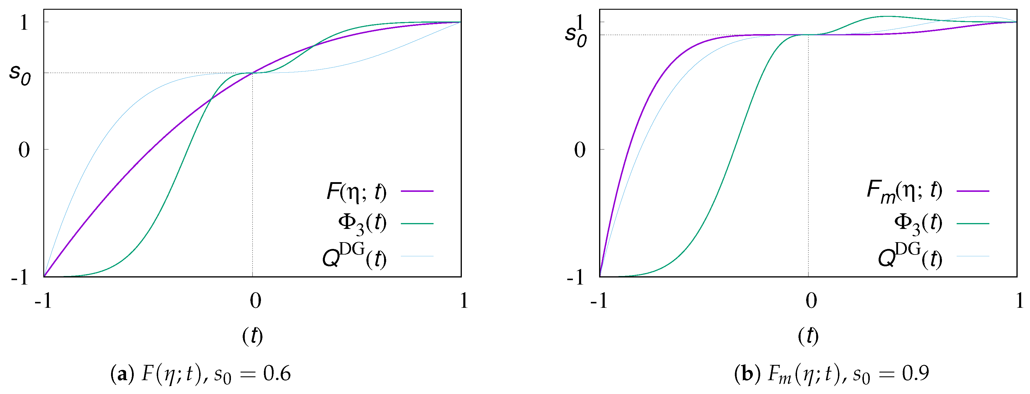
3.2. A New Composite Transformation

Set a quadratic function

$$g(\eta ;t)=\eta \left(1-t^2\right)+t,-1\le t\le 1,$$

(31)

which is a bijective function on $[-1,1]$ for $0\le \eta \le \frac{1}{2}$ and it satisfies

$$g(\eta ;-1)=-1,g(\eta ;0)=\eta ,g(\eta ;1)=1.$$

Next, we set a function $f(\eta ;t)=f_1(\eta ;t)$, i.e., from (11)

$$f(\eta ;t)=s_0+\left(1-s_{0}t\right)\frac{t-\eta }{1-\eta t},-1\le t\le 1.$$

(32)

The condition (14) with $m=1$ implies that the parameter $\eta$ should satisfy

$$\eta \ge -1+2s_0\left(0\le s_0<1\right).$$

(33)

Then we define a composite function

$$F(\eta ;t)=f\left(\eta ;g(\eta ;t)\right),-1\le t\le 1,$$

(34)

where it is assumed that $0\le \eta \le \frac{1}{2}$ for $g(\eta ;t)$ to be bijective on the interval $-1\le t\le 1$. This function satisfies the properties given in (26) as

$$F(\eta ;-1)=-1,F\left(\eta ;0\right)=s_0,F(\eta ;1)=1.$$

(35)

To choose a parameter $\eta$ satisfying the conditions $0\le \eta \le \frac{1}{2}$ and $\eta \ge -1+2s_0$ simultaneously we should suppose that $s_0$ is located in the interval

$$0\le s_0\le \frac{3}{4}$$

(36)

and in this case we may take $\eta$ such as, for example,

$${\eta }_1=\frac{2}{3}{s}_0\mathrm{or}{\eta }_2=\frac{8}{9}{s}_0^2.$$

(37)

That is, for any $0\le s_0\le \frac{3}{4}$ given, the function $F(\eta ;t)$ is bijective on the interval $[-1,1]$ if we take ${\eta }_1$ or ${\eta }_2$ for the parameter $\eta$. Figure 5a illustrates graphs of the proposed transformation $F(\eta ;t)$ with $\eta =\frac{2}{3}{s}_0$, the composite transformation ${\mathsf{\Phi }}_3\left(t\right)$ and the Doblaré-Gracia transformation $Q^{\mathrm{DG}}\left(t\right)$ for the cases of $s_0=0.6$.

If we change the variable $x=F(\eta ;t)$ in (25) then we may expect accurate numerical evaluation of the CPV integral by using a traditional Gauss quadrature rule with even number of integration points.

When $s_0>\frac{3}{4}$, on the other hand, from the inequality (14) we consider the following condition for the order m of $f_m(\eta ;t)$ instead of the condition (33) for $\eta$.

$$m\ge \left(\frac{1-\eta }{1+\eta }\right)\frac{s_0}{1-s_0}$$

(38)

for $0\le \eta \le \frac{1}{2}$ fixed. We will choose the value of m as small as possible. For example,

$$m=\left\{\begin{array}{cc}⌊\left(\frac{1-\eta }{1+\eta }\right)\frac{s_0}{1-s_0}⌋+1\hfill & \mathrm{if}⌊\left(\frac{1-\eta }{1+\eta }\right)\frac{s_0}{1-s_0}⌋\mathrm{is}\mathrm{even}\hfill \\ ⌊\left(\frac{1-\eta }{1+\eta }\right)\frac{s_0}{1-s_0}⌋+2\hfill & \mathrm{if}⌊\left(\frac{1-\eta }{1+\eta }\right)\frac{s_0}{1-s_0}⌋\mathrm{is}\mathrm{odd}\hfill \end{array}\right.,$$

(39)

where $\lfloor x\rfloor$ means the greatest integer less than or equal to x. Then, using the function $f_m(\eta ;t)$ in (11), we define a composite function

$$F_m(\eta ;t)=f_m\left(\eta ;g(\eta ;t)\right),-1\le t\le 1.$$

(40)

Figure 5b illustrates graphs of $F_m(\eta ;t)$ with $\eta =\frac{1}{3}$ and m chosen by (39), the composite transformation ${\mathsf{\Phi }}_3\left(t\right)$ and the Doblaré-Gracia transformation $Q^{\mathrm{DG}}\left(t\right)$ for the cases of $s_0=0.9$. For the case of $s_0>\frac{3}{4}$, in using the change of variable $x=F_m(\eta ;t)$ in (25), the formula (39) indicates that the higher order m is required as $s_0$ becomes close to the end-point $x=1$.

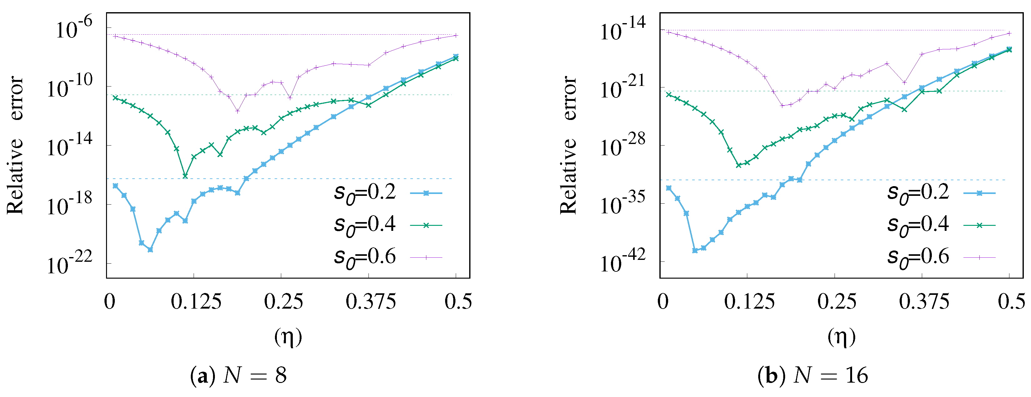
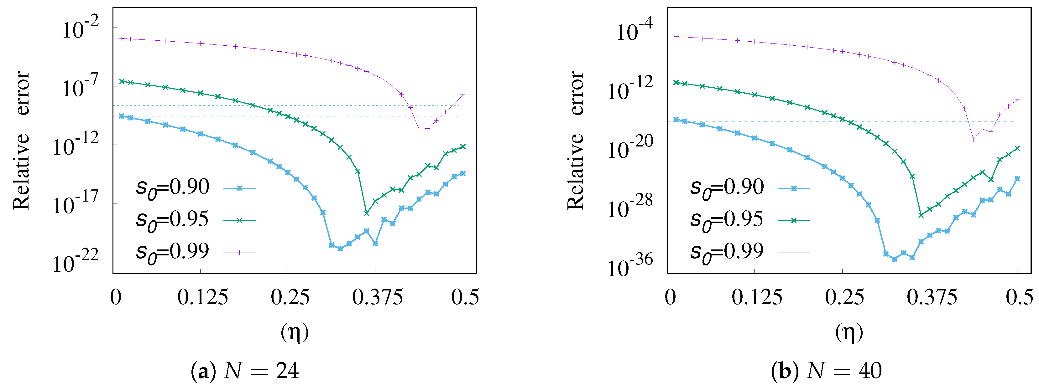
3.3. Numerical Examples

Example 3.

We take an example $K\varphi \left(s_0\right)$ with $\varphi \left(x\right)=1+x$ as follows.

$$K\varphi \left(s_0\right)=\mathrm{P}.\mathrm{V}.{\int }_{-1}^1\frac{1+x}{x-s_0}dx=2+\left(1+s_0\right)log\frac{1-s_0}{1+s_0}.$$

For $s_0=0.2,0.4,0.6$ within the interval given in (36), numerical results of the N-point Gauss-Legendre quadrature rule associated with the presented transformation $F(\eta ;t)$ are given in

Table 4. Relative errors of the N-point Gauss-Legendre quadrature rule corresponding to the Doblaré-Gracia transformation $Q^{\mathrm{DG}}\left(t\right)$ and the presented transformation $F(\eta ;t)$ for the CPV integral $K\varphi \left(s_0\right)$, $0\le s_0\le \frac{3}{4}$, in Example 3.

		Existing Transformation		Presented Transformation $\mathit{F}(\mathit{\eta };\mathit{t})$
${\mathit{s}}_{\mathbf{0}}$	$\mathit{N}$	${\mathit{Q}}^{\mathbf{DG}}\left(\mathit{t}\right)$		$\mathit{\eta }=\frac{\mathbf{2}}{\mathbf{3}}{\mathit{s}}_{\mathbf{0}}$	$\eta =\frac{\mathbf{8}}{\mathbf{9}}{\mathit{s}}_{\mathbf{0}}^{\mathbf{2}}$	$\eta =\frac{\mathbf{1}}{\mathbf{3}}{\mathit{s}}_{\mathbf{0}}$
0.2	4	$5.2\times {10}^{-9}$		$3.8\times {10}^{-9}$	$5.1\times {10}^{-10}$	$\mathbf{6.0}\times {\mathbf{10}}^{-\mathbf{11}}$
	8	$5.7\times {10}^{-17}$		$3.7\times {10}^{-18}$	$7.3\times {10}^{-19}$	$\mathbf{7.7}\times {\mathbf{10}}^{-\mathbf{21}}$
	12	$6.3\times {10}^{-25}$		$4.5\times {10}^{-27}$	$1.0\times {10}^{-27}$	$\mathbf{1.3}\times {\mathbf{10}}^{-\mathbf{30}}$
	16	$6.9\times {10}^{-33}$		$1.1\times {10}^{-36}$	$1.4\times {10}^{-36}$	$\mathbf{5.0}\times {\mathbf{10}}^{-\mathbf{41}}$
	20	$7.5\times {10}^{-41}$		$3.5\times {10}^{-44}$	$2.0\times {10}^{-45}$	$\mathbf{1.5}\times {\mathbf{10}}^{-\mathbf{50}}$
0.4	4	$7.6\times {10}^{-6}$		$2.1\times {10}^{-6}$	$\mathbf{1.7}\times {\mathbf{10}}^{-\mathbf{8}}$	$6.1\times {10}^{-8}$
	8	$2.8\times {10}^{-11}$		$1.9\times {10}^{-12}$	$7.6\times {10}^{-15}$	$\mathbf{1.7}\times {\mathbf{10}}^{-\mathbf{15}}$
	12	$1.0\times {10}^{-16}$		$1.4\times {10}^{-18}$	$2.4\times {10}^{-22}$	$\mathbf{1.7}\times {\mathbf{10}}^{-\mathbf{22}}$
	16	$3.7\times {10}^{-22}$		$3.8\times {10}^{-25}$	$1.4\times {10}^{-29}$	$\mathbf{7.6}\times {\mathbf{10}}^{-\mathbf{30}}$
	20	$1.3\times {10}^{-27}$		$4.9\times {10}^{-31}$	$1.3\times {10}^{-36}$	$\mathbf{1.7}\times {\mathbf{10}}^{-\mathbf{37}}$
0.6	4	$2.2\times {10}^{-3}$		$1.2\times {10}^{-4}$	$1.8\times {10}^{-4}$	$\mathbf{2.4}\times {\mathbf{10}}^{-\mathbf{5}}$
	8	$3.4\times {10}^{-7}$		$1.9\times {10}^{-8}$	$3.3\times {10}^{-9}$	$\mathbf{2.9}\times {\mathbf{10}}^{-\mathbf{11}}$
	12	$5.3\times {10}^{-11}$		$1.1\times {10}^{-12}$	$4.6\times {10}^{-14}$	$\mathbf{3.5}\times {\mathbf{10}}^{-\mathbf{17}}$
	16	$8.1\times {10}^{-15}$		$3.8\times {10}^{-17}$	$6.1\times {10}^{-19}$	$\mathbf{3.2}\times {\mathbf{10}}^{-\mathbf{23}}$
	20	$1.2\times {10}^{-18}$		$9.3\times {10}^{-22}$	$7.9\times {10}^{-24}$	$\mathbf{7.6}\times {\mathbf{10}}^{-\mathbf{30}}$

. Therein,

$$\eta =\frac{2}{3}{s}_0,\frac{8}{9}{s}_0^2,\frac{1}{3}{s}_0$$

are chosen for the parameter $\eta$. In the table we can see that $F(\eta ;t)$ provides better errors than the Doblaré-Gracia transformation $Q^{\mathrm{DG}}\left(t\right)$ defined in (29). By numerical experiment we can find that the other existing composite transformation ${\mathsf{\Phi }}_r\left(t\right)$ of any order $r>1$ gives worse errors than $Q^{\mathrm{DG}}\left(t\right)$.

For $s_0=0.9,0.95,0.99$, selected near the end-point $x=1$, numerical results of the N-point Gauss-Legendre quadrature rule associated with the presented transformation $F_m(\eta ;t)$, with m determined by the formula (39), are given in

Table 5. Relative errors of the N-point Gauss-Legendre quadrature rule corresponding to the composite transformation ${\mathsf{\Phi }}_3\left(t\right)$ and the presented transformation $F_m(\eta ;t)$ for the CPV integral $K\varphi \left(s_0\right)$, with $s_0$’s near the end-point, in Example 3.

		Existing Transformation		Presented Transformation ${\mathit{F}}_{\mathit{m}}(\mathit{\eta };\mathit{t})$
${\mathit{s}}_{\mathbf{0}}$	$\mathit{N}$	${{\Phi }}_{\mathbf{3}}\left(\mathit{t}\right)$		$\mathit{\eta }=\frac{\mathbf{1}}{\mathbf{2}}$	$\mathit{\eta }=\frac{\mathbf{1}}{\mathbf{3}}$	$\mathit{\eta }=\frac{\mathbf{1}}{\mathbf{4}}$
0.90	16	$6.6\times {10}^{-7}$		$4.1\times {10}^{-10}$	$\mathbf{8.0}\times {\mathbf{10}}^{-\mathbf{15}}$	$3.1\times {10}^{-10}$
	24	$2.8\times {10}^{-10}$		$3.6\times {10}^{-15}$	$\mathbf{2.6}\times {\mathbf{10}}^{-\mathbf{21}}$	$4.3\times {10}^{-15}$
	32	$1.0\times {10}^{-13}$		$1.7\times {10}^{-20}$	$\mathbf{2.9}\times {\mathbf{10}}^{-\mathbf{28}}$	$6.0\times {10}^{-20}$
	40	$3.6\times {10}^{-17}$		$6.7\times {10}^{-25}$	$\mathbf{1.3}\times {\mathbf{10}}^{-\mathbf{35}}$	$8.3\times {10}^{-25}$
	48	$1.1\times {10}^{-20}$		$4.8\times {10}^{-30}$	$\mathbf{1.4}\times {\mathbf{10}}^{-\mathbf{42}}$	$1.1\times {10}^{-29}$
0.95	16	$3.6\times {10}^{-6}$		$1.7\times {10}^{-8}$	$\mathbf{3.3}\times {\mathbf{10}}^{-\mathbf{9}}$	$4.5\times {10}^{-7}$
	24	$2.1\times {10}^{-9}$		$6.9\times {10}^{-13}$	$\mathbf{1.7}\times {\mathbf{10}}^{-\mathbf{13}}$	$2.6\times {10}^{-10}$
	32	$5.1\times {10}^{-12}$		$2.7\times {10}^{-17}$	$\mathbf{8.9}\times {\mathbf{10}}^{-\mathbf{18}}$	$1.4\times {10}^{-13}$
	40	$1.9\times {10}^{-15}$		$9.4\times {10}^{-21}$	$\mathbf{4.6}\times {\mathbf{10}}^{-\mathbf{22}}$	$8.1\times {10}^{-17}$
	48	$7.1\times {10}^{-18}$		$1.2\times {10}^{-24}$	$\mathbf{2.4}\times {\mathbf{10}}^{-\mathbf{26}}$	$4.6\times {10}^{-20}$
0.99	16	$\mathbf{6.0}\times {\mathbf{10}}^{-\mathbf{6}}$		$8.8\times {10}^{-6}$	$3.6\times {10}^{-4}$	$1.7\times {10}^{-3}$
	24	$5.8\times {10}^{-7}$		$\mathbf{1.8}\times {\mathbf{10}}^{-\mathbf{8}}$	$6.9\times {10}^{-6}$	$7.1\times {10}^{-5}$
	32	$3.5\times {10}^{-9}$		$\mathbf{3.0}\times {\mathbf{10}}^{-\mathbf{11}}$	$1.3\times {10}^{-7}$	$2.9\times {10}^{-6}$
	40	$3.4\times {10}^{-12}$		$\mathbf{3.4}\times {\mathbf{10}}^{-\mathbf{14}}$	$2.4\times {10}^{-9}$	$1.1\times {10}^{-7}$
	48	$1.8\times {10}^{-13}$		$\mathbf{2.8}\times {\mathbf{10}}^{-\mathbf{18}}$	$4.4\times {10}^{-11}$	$4.5\times {10}^{-9}$

. The parameter $\eta$ is chosen by $\eta =\frac{1}{2},\frac{1}{3},\frac{1}{4}.$ The table includes numerical results of the existing composite transformation ${\mathsf{\Phi }}_r\left(t\right)$ in (30) associated with the Sidi-sigmoidal transformation ${\gamma }_r\left(\tau \right)={\gamma }_r^{\mathrm{Sidi}}\left(\tau \right)$ defined as

$${\gamma }_r^{\mathrm{Sidi}}\left(\tau \right)=\frac{1}{q_r}{\int }_0^{\tau }{sin}^{r-1}\left(\pi y\right)dy,$$

(41)

where

$$q_r={\int }_0^1{sin}^{r-1}\left(\pi y\right)dy.$$

By the numerical experiment we can find that ${\mathsf{\Phi }}_r\left(t\right)$ of order $r=3$ results in better errors than $Q^{\mathrm{DG}}\left(t\right)$ and ${\mathsf{\Phi }}_r\left(t\right)$ of any order $r\ne 3$. Thus, Table 5 includes numerical results of ${\mathsf{\Phi }}_3\left(t\right)$. The table shows the superiority of the proposed transformation $F_m(\eta ;t)$, with $\eta =\frac{1}{2},\frac{1}{3}$, compared with the existing composite transformation ${\mathsf{\Phi }}_3\left(t\right)$. In addition,

Table 6. Values of m evaluated by Equation (39) for each $s_0$ and $\eta$ selected in Table 5.

		m
${\mathit{s}}_{\mathbf{0}}$		$\mathit{\eta }=\frac{\mathbf{1}}{\mathbf{2}}$	$\mathit{\eta }=\frac{\mathbf{1}}{\mathbf{3}}$	$\mathit{\eta }=\frac{\mathbf{1}}{\mathbf{4}}$
0.90		5	5	7
0.95		7	11	13
0.99		33	51	61

shows the values of m evaluated by (39) for each $s_0$ and $\eta$ selected in Table 5. Moreover, Figure 6 and Figure 7 respectively show the behaviors of the relative errors of $F(\eta ;t)$ for $0\le s_0\le \frac{3}{4}$ and those of $F_m(\eta ;t)$ for $s_0>\frac{3}{4}$ over the range $0\le \eta \le \frac{1}{2}$. In particular, from Figure 7 one can see that the region of the parameter $\eta$ providing splendid errors will move toward the right as $s_0$ becomes close to the end-point $x=1$.

4. Conclusions

In this work we proposed rational transformations of simple forms for evaluation of singular integrals by the Gauss-Legendre quadrature rule. We summarize this work for each type of the singular integral as follows.

i.

Interior-point weakly singular integrals: The rational transformation $f_m(\eta ;t)$ in (11) is proposed. Numerical evaluation based on the proposed rational transformation does not require any division of the integration interval, and its numerical results are comparable to the existing transformations.

ii.

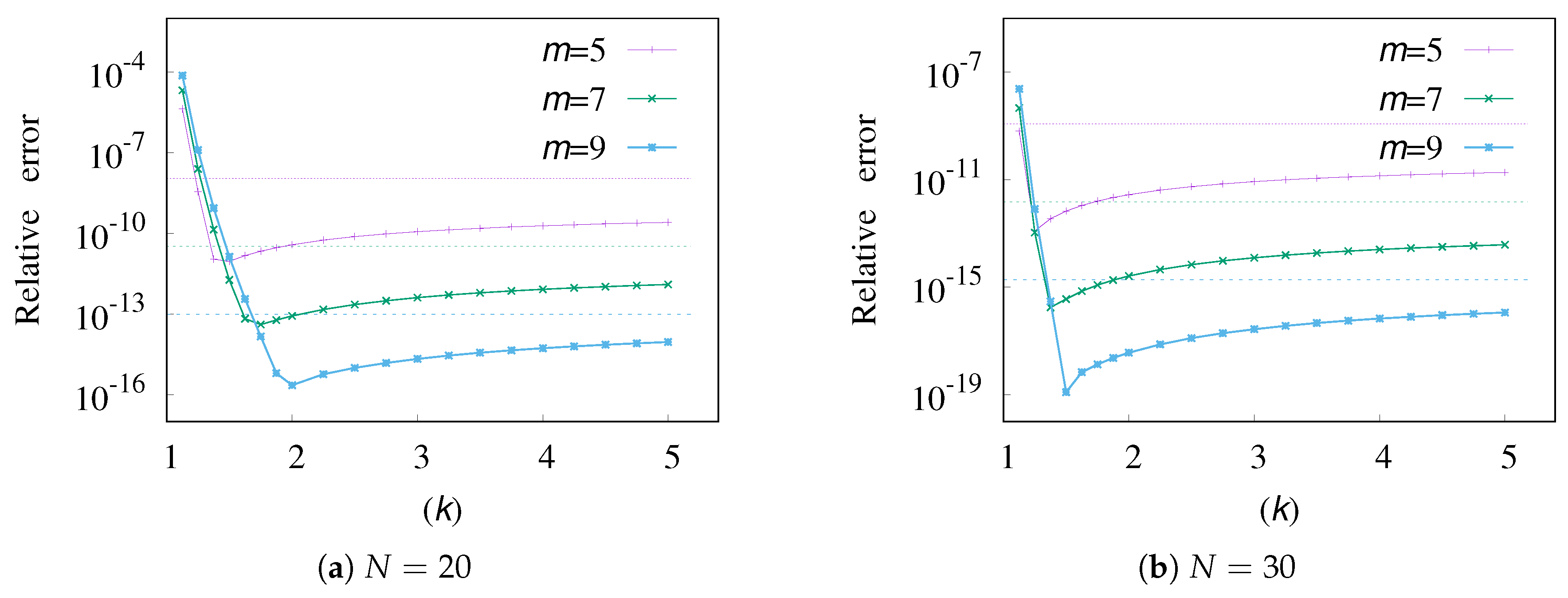
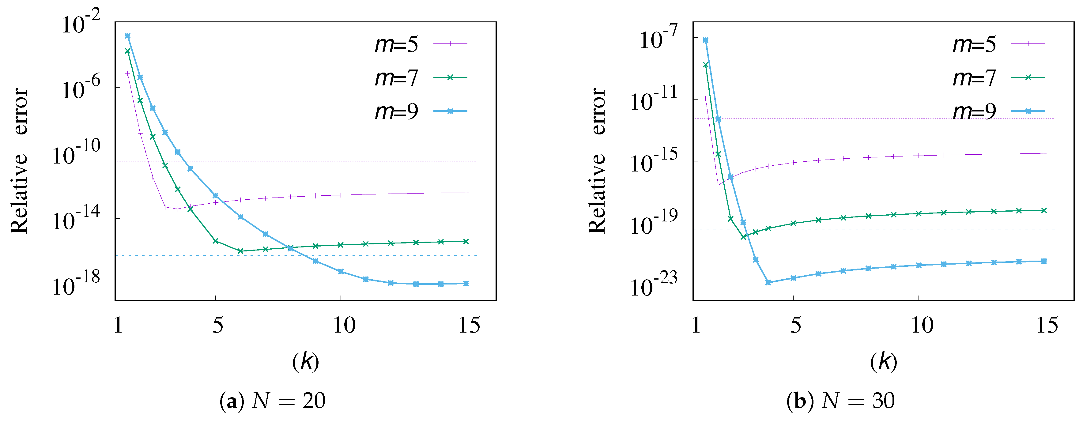
End-point weakly singular integrals: The rational transformation ${\tilde{f}}_m(k;t)$ in (15) is proposed and it provides better errors than the exiting transformations when an appropriate value of k is selected.

iii.

Cauchy principal value integrals: The composite rational transformations, $F(\eta ;t)$ in (34) for the singular point $0\le s_0\le \frac{3}{4}$ and $F_m(\eta ;t)$ in (40) for the near end singular point $\frac{3}{4}<s_0<1$ are suggested. The proposed rational transformations, with appropriate values of $\eta$ and m, produce splendid results.

We have experimentally identified suitable intervals of the parameters in the proposed rational transformations without complete theoretical investigation, and we leave it as another problem to perform in a further work.

References

1. Doblaré, M. Computational aspects of the boundary element methods. In Topics in Boundary Element Research; Springer: Berlin, Germany, 1987; Volume 3. [Google Scholar]
2. Kythe, P.K. An Introduction to Boundary Element Method; CRC Press: Boca Raton, FL, USA, 1995. [Google Scholar]
3. Ma, Y.; Huang, J. Asymptotic error expansions and splitting extrapolation algorithm for two classes of two-dimensional Cauchy principal-value integrals. Appl. Math. Comput. 2019, 357, 107–118. [Google Scholar] [CrossRef]
4. Qiu, Z.H.; Wrobel, L.C.; Power, H. Numerical solution of convection-diffusion problems at high Peclét number using boundary elements. Int. J. Numer. Methods Eng. 1998, 41, 899–914. [Google Scholar] [CrossRef]
5. Savruk, M.P.; Kazberuk, A. Method of Singular Integral Equations in Application to Problems of the Theory of Elasticity. In Stress Concentration at Notches; Springer: Cham, Switzerland, 2017; pp. 1–56. [Google Scholar]
6. Doblaré, M.; Gracia, L. On non-linear transformations for integration of weakly-singular and Cauchy principal value integrals. Int. J. Numer. Methods Eng. 1997, 40, 3325–3358. [Google Scholar] [CrossRef]
7. Elliott, D. The cruciform crack problem and sigmoidal transformations. Math. Methods Appl. Sci. 1997, 20, 121–132. [Google Scholar] [CrossRef]
8. Elliott, D. The Euler Maclaurin formula revised. J. Austral. Math. Soc. Ser. B 1998, 40, E27–E76. [Google Scholar]
9. Elliott, D.; Venturino, E. Sigmoidal transformations and the Euler-Maclaurin expansion for evaluating certain Hadamard finite-part integrals. Numer. Math. 1997, 77, 453–465. [Google Scholar] [CrossRef]
10. Johnston, P.R. Semi-sigmoidal transformations for evaluating weakly singular boundary element integrals. Int. J. Numer. Methods Eng. 2000, 47, 1709–1730. [Google Scholar] [CrossRef]
11. Johnston, P.R.; Elliott, D. Error estimation of quadrature rules for evaluating singular integrals in boundary element. Int. J. Numer. Methods Eng. 2000, 48, 949–962. [Google Scholar] [CrossRef]
12. Johnston, P.R.; Elliott, D. A generalization of Telles’ method for evaluating weakly singular boundary element integrals. J. Comput. Appl. Math. 2001, 131, 223–241. [Google Scholar] [CrossRef]
13. Sanz Serna, J.M.; Doblaré, M.; Alarcon, E. Remarks on methods for the computation of boundary-element integrals by co-ordinate transformation. Commun. Appl. Numer. Methods 1990, 6, 121–123. [Google Scholar] [CrossRef] [Green Version]
14. Sato, M.; Yoshiyoka, S.; Tsukui, K.; Yuuki, R. Accurate numerical integration of singular kernels in the two-dimensional boundary element method. In Boundary Elements X; Brebbia, C.A., Ed.; Springer: Berlin, Germany, 1988; Volume 1, pp. 279–296. [Google Scholar]
15. Telles, J.C.F. A self-adaptive co-ordinate transformation for efficient numerical evaluation of general boundary element integrals. Int. J. Numer. Methods Eng. 1987, 24, 959–973. [Google Scholar] [CrossRef]
16. Yun, B.I. An extended sigmoidal transformation technique for evaluating weakly singular integrals without splitting the integration interval. SIAM J. Sci. Comput. 2003, 25, 284–301. [Google Scholar] [CrossRef]
17. Yun, B.I. A composite transformation for numerical integration of singular integrals in the BEM. Int. J. Numer. Methods Eng. 2003, 57, 1883–1898. [Google Scholar] [CrossRef]
18. Yun, B.I. A generalized non-linear transformation for evaluating singular integrals. Int. J. Numer. Methods Eng. 2006, 65, 1947–1969. [Google Scholar] [CrossRef]
19. Monegato, G.; Sloan, I.H. Numerical solutions of the generalized airfoil equation for an airfoil with a flap. SIAM J. Numer. Anal. 1997, 34, 2288–2305. [Google Scholar] [CrossRef]
Figure 1. Graphs of the proposed rational transformations f m ( η ; t ) , η = s 0 , with respect to m = 3 , 5 , 7 in (a) and graphs of f 3 ( η ; t ) with respect to η 1 = s 0 , η 2 = s 0 / 2 , η 3 = s 0 / 4 in (b) for the case of s 0 = 0.65 .
Mathematics 08 00677 g001
Figure 2. Graphs of the proposed rational transformations f ˜ 3 ( k ; t ) , k = 2 , 5 , 100 , compared with γ ˜ 3 ( t ) (: dotted line) and P 3 Sat ( t ) (: solid line).
Mathematics 08 00677 g002
Figure 3. Relative errors of f ˜ m ( k ; t ) , 1 < k < 5 , for the end-point weakly singular integral I α ϕ ( ξ 0 ) , with α = 0.45 and ξ 0 = 1 , in Example 2. Dotted horizontal lines indicate relative errors of P m Sat ( t ) for m = 5 , 7 , 9 from top to bottom.
Mathematics 08 00677 g003
Figure 4. Relative errors of f ˜ m ( k ; t ) , 1 < k < 15 , for the end-point logarithmic singular integral J ϕ ( ξ 0 ) , with ξ 0 = 1 , in Example 2. Dotted horizontal lines indicate relative errors of P m Sat ( t ) for m = 5 , 7 , 9 from top to bottom.
Mathematics 08 00677 g004
Figure 5. Graphs of the proposed rational transformation F ( η ; t ) , with η = 2 3 s 0 , for s 0 = 0.6 in (a) and graphs of F m ( η ; t ) , with η = 1 3 and m chosen by (39), for s 0 = 0.9 in (b) compared with the composite transformation Φ 3 ( t ) and the Doblaré-Gracia transformation Q D G ( t ) .
Mathematics 08 00677 g005
Figure 6. Relative errors of F ( η ; t ) , 0 < η < 1 2 , for the CPV integral K ϕ ( s 0 ) , for s 0 = 0.2 , 0.4 , 0.6 , in Example 3. Dotted horizontal lines indicate relative errors of Q DG ( t ) corresponding to the chosen values of s 0 .
Mathematics 08 00677 g006
Figure 7. Relative errors of F m ( η ; t ) , 0 < η < 1 2 , for the CPV integral K ϕ ( s 0 ) , for s 0 = 0.9 , 0.95 , 0.99 , in Example 3. Dotted horizontal lines indicate relative errors of Φ 3 ( t ) corresponding to the chosen values of s 0 .
Mathematics 08 00677 g007