Statistical Analysis of a Lifetime Distribution with a Bathtub-Shaped Failure Rate Function under Adaptive Progressive Type-II Censoring

Abstract

In this paper, the estimation problem of two parameters of a lifetime distribution with a bathtub-shaped failure rate function based on adaptive progressive type-II censored data is discussed. This censoring scheme allows the experiment to be more efficient in the use of time and cost while ensuring the statistical inference efficiency based on the experimental results. Maximum likelihood estimators are proposed and the approximate confidence intervals for two parameters are computed using the asymptotic normality. Lindley approximation and Gibbs sampling are used to obtain Bayes point estimates and the latter is also used to generate Bayes two-sided credible intervals. Finally, the performance of various estimation methods is evaluated through simulation experiments, and the proposed estimation method is illustrated through the analysis of a real data set.

1. Introduction

1.1. Chen$(\beta ,\theta )$ Distribution

In practical analysis, the failure rate function is the key for researchers to study the life phenomenon of a product. In many industries, products are more likely to have a bathtub-shaped failure rate curve than a fixed failure rate. For the bathtub-shaped failure rate function, the product failure rate begins with a decreasing process, then a constant phase, and finally an ascending phase. This model has wide application prospects. For example, some treatments or drugs may work better in middle-aged men than in other age groups. That is, the failure rate of the treatment for children is high, and it will continue to fall to a constant level, then it will maintain that constant level until a certain age, later will rise again as the growth of the age gradually. The exponentiated Weibull extension proposed by Chen [1] (written as Chen$(\beta ,\theta )$ distribution and abbreviated as the Chen distribution throughout the paper) is a lifetime distribution with bathtub-shaped failure rate function. The confidence regions of the two unknown parameters of the Chen$(\beta ,\theta )$ distribution have closed forms, which are important for practical applications. Chen [1] proposed an exact confidence interval for two parameters based on type-II censored data. Many researchers have also been interested in this new lifetime distribution and have conducted a series of studies. Based on the same censored data, Wang [2] explored some analytical properties of this distribution, added moment estimation, and evaluated the performance of the proposed estimation methods through intensive Monte Carlo simulations. Sanku Dey [3] focused on frequentist analyses and Mohammad Z Raqab [4] further studied bayesian analyses with the record data. Under the progressive type-II censored data, Wu [5] proposed maximum likelihood estimation and a method to construct exact confidence intervals as well as exact joint confidence regions of parameters. Manoj Kumar Rastogi [6] further discussed the estimation of its reliability function as well as hazard function based on the same censoring scheme. Bahman Tarvirdizade [7] considered the estimation of the stress-strength reliability based on upper record values. Essam Kh Ahmed [8] further used the Markov Chain Monte Carlo method (MCMC) for Bayes estimation with the progressive type-II censored data. Zhang [9] discussed acceleration factors based on the tampered failure rate model.

The probability density function (pdf) of Chen$(\beta ,\theta )$ is given by

$$f(x;\beta ,\theta )=\frac{\beta }{\theta }·x^{\beta -1}·e^{x^{\beta }}·exp(\frac{1-e^{x^{\beta }}}{\theta }),x>0$$

(1)

and cumulative distribution function (cdf) is

$$F(x;\beta ,\theta )=1-exp(\frac{1-e^{x^{\beta }}}{\theta }),x>0,$$

(2)

where $\beta >0,\theta >0$ are the parameters.

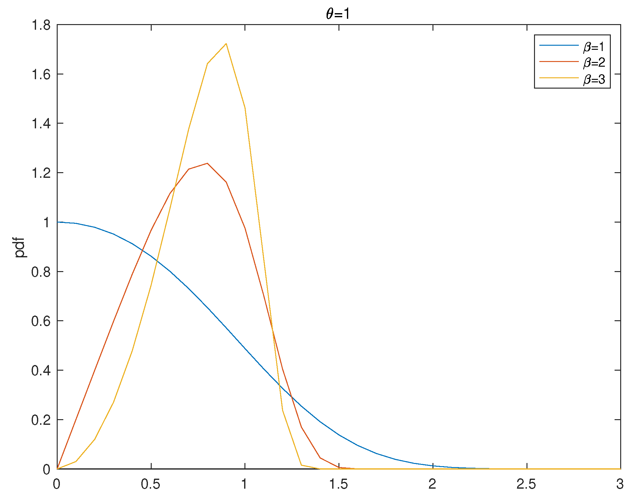
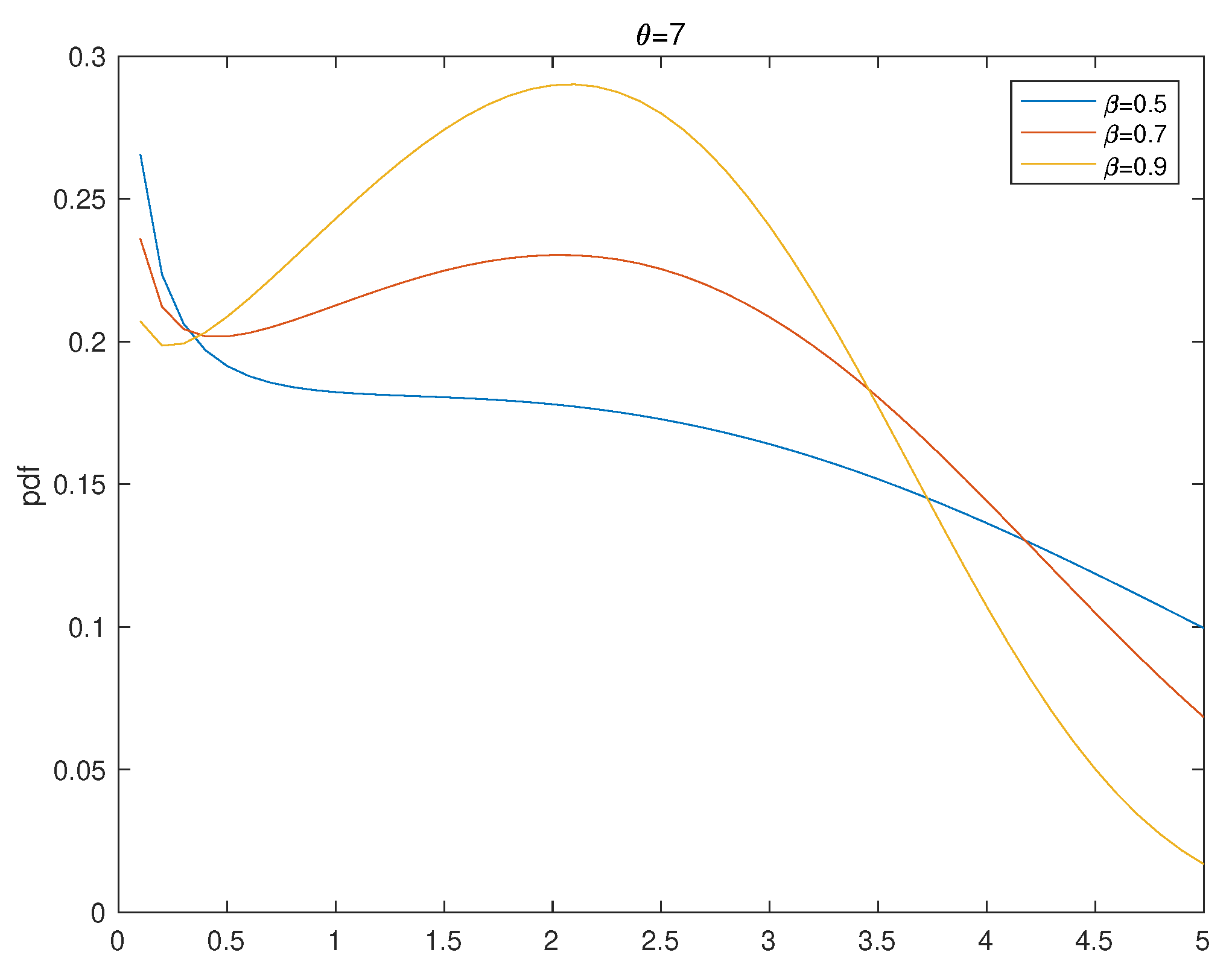
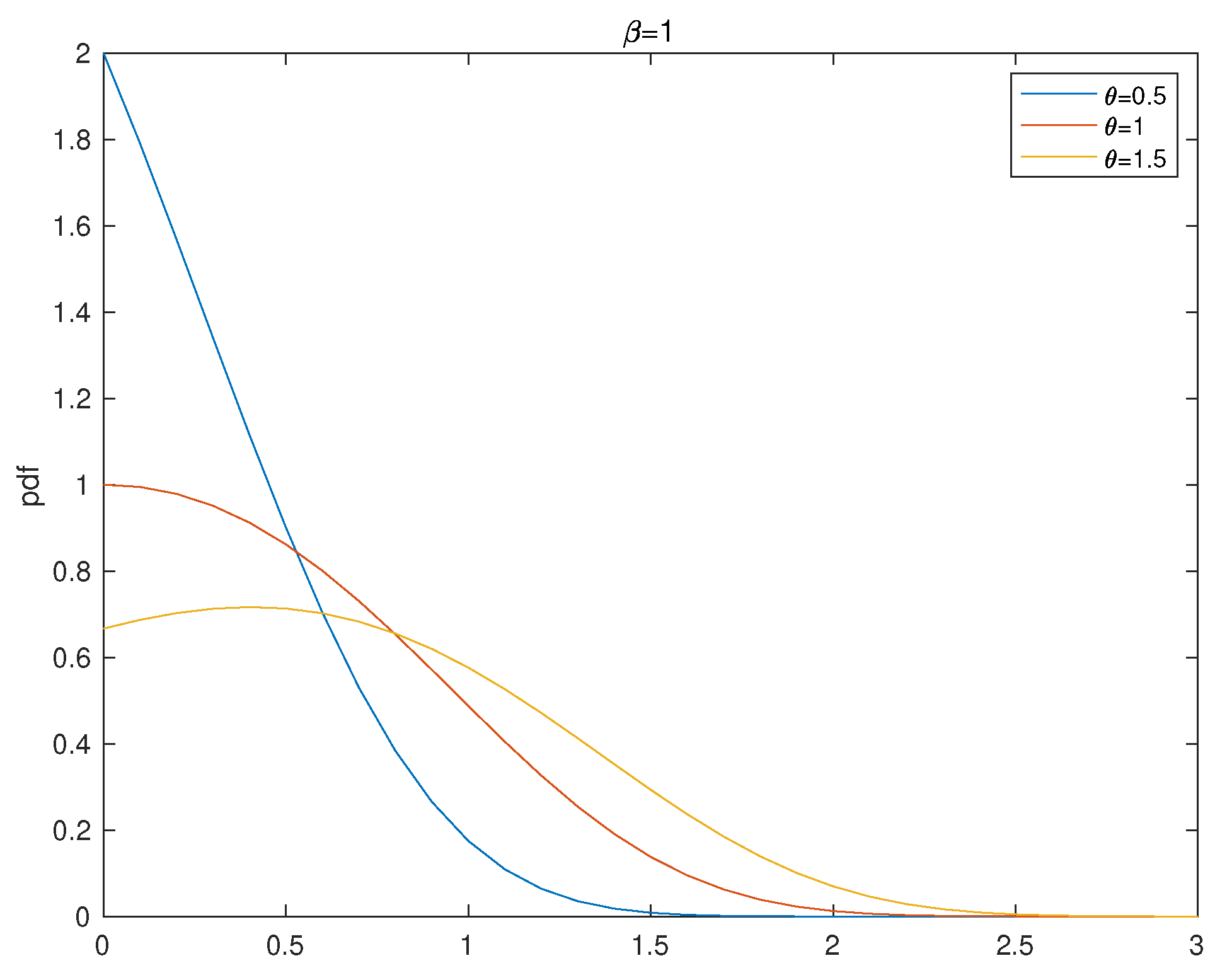
Some of its characteristics are illustrated below. $f(x)$ is decreasing for $0<\theta \le 1$, $\beta \le 1$; $f(x)$ is unimodal for $\beta >1$. When $\theta >1$, $f(x)$ is either decreasing, or decreasing first and then increasing and decreasing finally (see [2] in details). Figure 1, Figure 2, Figure 3 and Figure 4 illustrate the curves of $f(x)$ under several settings of two parameter values.

Figure 1. The probability density function (pdf) when $\beta =1$, $0<\theta \le 1$.

Figure 2. The pdf when $\beta <1$, $0<\theta \le 1$.

Figure 3. The pdf when $\beta >1$, $0<\theta \le 1$.

Figure 4. The pdf when $\beta \le 1$, $\theta >1$.

The failure rate function of the Chen$(\beta ,\theta )$ is

$$\lambda (x)=(\frac{\beta }{\theta })·x^{\beta -1}·e^{x^{\beta }}.$$

(3)

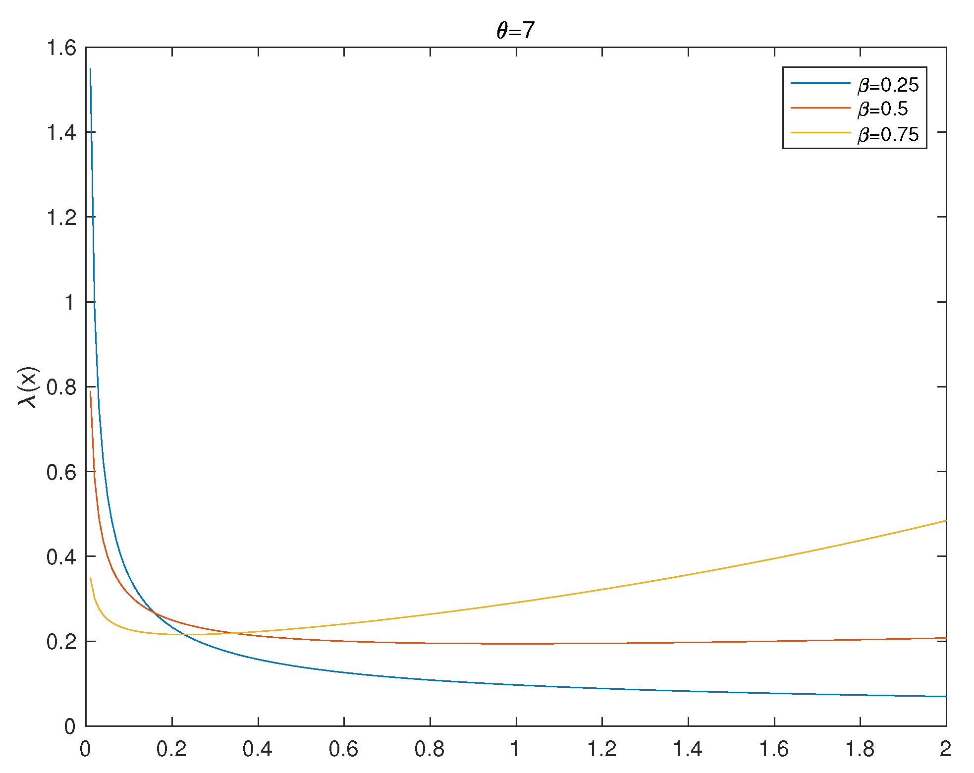
Taking the derivation, ${\lambda }^{\prime }(x)=\frac{\beta }{\theta }·x^{\beta -2}·e^{x^{\beta }}·\left[(\beta -1)+\beta x^{\beta }\right]$, from which we can conclude that $\lambda (x)$ is in a bathtub-shaped curve when $0<\beta <1$ and increases when $\beta \ge 1$. Figure 5 and Figure 6 show the curves of $\lambda (x)$ under various settings of $\beta$ and $\theta$. Since the failure rate at the bottom of the bathtub is stable, which is closely related to the working stage of the actual product, it is of great significance to analyze this kind of lifetime distribution for the practical application in industry.

Figure 5. $\lambda (x)$ when $\theta =7$, $0<\beta <1$.

Figure 6. $\lambda (x)$ when $\theta =1$, $\beta \ge 1$.

1.2. Adaptive Progressive Type-II Censored Scheme

In the life test and reliability test, the experimenters use various censoring schemes to reduce the total test time and related costs among which type-II censoring scheme is one of the most widely used. Under type-II censoring scheme, only the first m failed units in a random sample in size n ($m<n$) are observed. This method is easy to be carried out by people, while it has the possibility of wasting a lot of testing time. Therefore, the progressive type-II censoring as a generalized form of type-II censoring is proposed to improve the efficiency of the experiment. The progressive type-II censoring can be implemented as follows. Let n units be placed on a life test and denote $X_1,X_2,\cdots ,X_n$ as their lifetimes, respectively. It is suppose that $X_i,i=1,2,\dots ,n$ are independent to each other and all follow pdf $f(x)$ and cdf $F(x)$. Before the experiment begins, the number of units observed m ($m<n$) as well as the progressive type-II censoring scheme $R=(R_1,R_2,\cdots ,R_m)$ are determined where $R_i>0,i=1,2,\cdots ,m$ and ${\sum }_{i=1}^m{R}_i+m=n$. When i-th failure is observed, the surviving $R_i$ units are randomly removed from the experiment. The experiment continues according to this rule until m failures are observed and the experiment is over.

Denote by m the completely observed lifetimes by $X_{i:m:n}^R,i=1,2,\cdots ,m$ (simplified to $X_{i:m:n}$ in a specific experiment), which are the observed progressive type-II right censoring order statistics. A basic assumption of the design of this experiment is that the censoring scheme $R=(R_1,R_2,\cdots ,R_m)$ is set before the experiment begins. This model can simulate the real-life situation where the loss or removal of some units happens during the experiment, which makes it more reasonable than type-II censoring.

However, this method may still fail to be satisfied in reality since experimenters may want to change the censoring numbers according to the actual situation during the experiment process. Thus, adaptive progressive type-II censoring is proposed [10] to improve the flexibility and efficiency of the experiment. In the adaptive progressive type-II censoring scheme, the size of units m observed is decided before the experiment and the censoring scheme $R=(R_1,R_2,\cdots ,R_m)$ is roughly decided, but $R_i$ may be modified according to certain needs of experimenters. The working process is demonstrated as follows: suppose there is a pre-provided expected finishing time T of the test, though we allow the total testing time to exceed T. If $X_{m:m:n}<T$, the experiment is carried out in the same way as type-II progressive censoring. Otherwise, once the experiment time pass time T while we have not observed m failures, we leave as many surviving units as possible, hoping to see more failures in a short time to finish the experiment in the most efficient way. Therefore, suppose $X_{J:m:n}$ is the last failure observed before time T (i.e., $X_{J:m:n}<T<X_{J+1:m:n})$ where $X_{0:m:n}\equiv 0$ and $X_{m+1:m:n}\equiv \infty$. After time T, we do not drop any units until the m-th failure is observed. Then we withdraw all surviving units. That is to say, $R_{J+1}=R_{J+2}=\cdots =R_{m-1}$=0 and $R_m=n-m-{\sum }_{i=1}^J{R}_i$. Figure 7 and Figure 8 illustrate progressive type-II censoring and adaptive progressive type-II censoring, respectively.

Figure 7. Progressive type-II censoring scheme.

Figure 8. Adaptive progressive type-II censoring scheme.

Based on adaptive type-II progressively censored data, the maximum likelihood estimation and Bayes estimation for two parameters of Chen$(\beta ,\theta )$ distribution have been studied. The rest of this paper is organized as follows. Maximum likelihood point estimation is considered and asymptotic confidence intervals using the asymptotic normality are constructed in Section 2. Then in Section 3, we discuss Bayes estimation and obtain numerical results to Bayes point estimators using Lindley approximation and Gibbs sampling. Furthermore, the latter is used to construct Bayes two-sided credible intervals of unknown parameters. In Section 4, the R program is used for simulation study to compare different estimation methods. In Section 5, a real data set is analyzed to demonstrate the feasibility of the proposed estimation methods. Finally, the thesis is summarized in the Section 6.

2. Maximum Likelihood Estimation

Suppose that $X=X_{1:m:n}^R,X_{2:m:n}^R,\cdots ,X_{m:m:n}^R$ is an adaptive progressive type-II censored sample of size m from a sample of size n with censoring scheme $R=(R_1,R_2,\cdots ,R_m)$ taken from distribution having $f(x)$ as the pdf and $F(x)$ as the cdf, and $X_{J:m:n}$ is the last observed failure before T which is prefixed best testing time. The parameter $x=x_{1:m:n}^R,x_{2:m:n}^R,\cdots ,x_{m:m:n}^R$ (simplified as $x=x_1,x_2,\cdots ,x_m$ in later equations) is used to represent the observed values of such an adaptive type-II progressively censored sample. On this basis, the corresponding likelihood function is given by

$$f(x_{1:m:n}^R,x_{2:m:n}^R,\dots ,x_{m:m:n}^R)=B_J·\left[\prod _{i=1}^{m}f(x_{i:m:n})\right]·\left[\prod _{i=1}^J{[1-F(x_{i:m:n})]}^{R_i}\right]·{\left[1-F(x_{m:m:n})\right]}^{C_J},$$

(4)

where $B_J={\prod }_{i=1}^m[n-i+1-{\sum }_{k=1}^{max(i-1,J)}{R}_k]$ and $C_J=n-m-{\sum }_{i=1}^J{R}_i$.

Therefore, the likelihood function for $X_{1:m:n}^R,X_{2:m:n}^R,\dots ,X_{m:m:n}^R$ taken from the Chen$(\beta ,\theta )$ is correspondingly written as

$$L\left(\beta ,\theta \mid x\right)=B_J·\frac{{\beta }^m}{{\theta }^m}·\prod _{i=1}^m\left[x_i^{\beta -1}·e^{x_i^{\beta }}·exp(\frac{1-e^{x_i^{\beta }}}{\theta })\right]·\prod _{i=1}^J{\left[exp(\frac{1-e^{x_i^{\beta }}}{\theta })\right]}^{R_i}·{\left[exp(\frac{(1-e^{x_m^{\beta }}}{\theta })\right]}^{C_J}.$$

(5)

Further, the log-likelihood function can then be written as

$$\begin{array}{ccc}\hfill l(\beta ,\theta \mid x)& =& mln\beta -mln\theta +\sum _{i=1}^m\left[(\beta -1)ln{x}_i+x_i^{\beta }+(\frac{1-e^{x_i^{\beta }}}{\theta })\right]\hfill \\ & & +\sum _{i=1}^J\left[R_i·(\frac{1-e^{x_i^{\beta }}}{\theta })\right]+C_J(\frac{1-e^{x_m^{\beta }}}{\theta }).\hfill \end{array}$$

(6)

Then take the partial derivatives of the log-likelihood function, and obtain the likelihood equations as follows:

$$\frac{\partial l(\beta ,\theta \mid x)}{\partial \beta }=\frac{m}{\beta }+\sum _{i=1}^m\left[ln{x}_i(1+x_i^{\beta }-x_i^{\beta }·\frac{e^{x_i^{\beta }}}{\theta })\right]-\sum _{i=1}^{J}ln{x}_i(x_i^{\beta }·R_i·\frac{e^{x_i^{\beta }}}{\theta })-ln{x}_m·x_m^{\beta }·C_J·\frac{e^{x_m^{\beta }}}{\theta }=0.$$

(7)

$$\frac{\partial l(\beta ,\theta \mid x)}{\partial \theta }=-\frac{m}{\theta }-\sum _{i=1}^m\frac{1-e^{x_i^{\beta }}}{{\theta }^2}-\sum _{i=1}^J\frac{R_i·(1-e^{x_i^{\beta }})}{{\theta }^2}-C_J·\frac{1-e^{x_m^{\beta }}}{{\theta }^2}=0.$$

(8)

From (8), the maximum likelihood estimate of $\theta$ can be illustrated as a function of $\widehat{\beta }$

$$\widehat{\theta }=-\frac{{\sum }_{i=1}^m(1-e^{x_i^{\widehat{\beta }}})+{\sum }_{i=1}^J{R}_i·(1-e^{x_i^{\widehat{\beta }}})+C_J·(1-e^{x_i^{\widehat{\beta }}})}{m}.$$

(9)

Thus, given $\widehat{\beta }$, the corresponding $\widehat{\theta }$ with (9) can be obtained. However, we cannot get the closed forms of (7) and (9). Therefore, numerical methods are included, such as Newton’s method, to determine the expected estimates.

Further, asymptotic confidence intervals are discussed. When the sample size n is large enough, the Fisher information matrix can be involved to get approximate confidence intervals of two unknown parameters. The Fisher information matrix is derived based on likelihood functions. By formula derivation, the pivot quantities with unknown parameters subject to asymptotically normal distribution are constructed. Then the asymptotic confidence intervals are obtained through Monte Carlo simulations.

The Fisher information matrix $I(\beta ,\theta )$ is written as

$$\begin{array}{c}\hfill I(\beta ,\theta )=E[-\left[\begin{array}{cc}\frac{{\partial }^{2}l(\beta ,\theta \mid x)}{{\partial }^2\beta }& \frac{{\partial }^{2}l(\beta ,\theta \mid x)}{\partial \beta \partial \theta }\\ \frac{{\partial }^{2}l(\beta ,\theta \mid x)}{\partial \theta \partial \beta }& \frac{{\partial }^{2}l(\beta ,\theta \mid x)}{{\partial }^2\theta }\end{array}\right]],\end{array}$$

(10)

and from the log-likelihood function (6), we have the second partial of $l(\beta ,\theta \mid x)$ with respect to $\beta$ and $\theta$ which is illustrated in the Appendix A.

It is obvious that it is difficult to get the exact expression of the above expectation. Therefore, the observed Fisher information matrix without taking expectation will be used instead. Let $(\widehat{\beta },\widehat{\theta })$ represent the maximum likelihood estimate of $(\beta ,\theta )$, the observed Fisher information matrix $I(\widehat{\beta },\widehat{\theta })$ is given as follows:

$$\begin{array}{c}\hfill I(\widehat{\beta },\widehat{\theta })={\left[\begin{array}{cc}-\frac{{\partial }^{2}l(\beta ,\theta \mid x)}{{\partial }^2\beta }& -\frac{{\partial }^{2}l(\beta ,\theta \mid x)}{\partial \beta \partial \theta }\\ -\frac{{\partial }^{2}l(\beta ,\theta \mid x)}{\partial \theta \partial \beta }& -\frac{{\partial }^{2}l(\beta ,\theta \mid x)}{{\partial }^2\theta }\end{array}\right]}_{\widehat{\beta }\widehat{\theta }}.\end{array}$$

(11)

Correspondingly, an approximated covariance matrix of $(\widehat{\beta },\widehat{\theta })$ is given as follows:

$$\begin{array}{c}\hfill \left[\begin{array}{cc}var(\widehat{\beta })& cov(\widehat{\beta },\widehat{\theta })\\ cov(\widehat{\theta },\widehat{\beta })& var(\widehat{\theta })\end{array}\right]=I^{-1}(\widehat{\beta },\widehat{\theta })={\left[\begin{array}{cc}-\frac{{\partial }^{2}l(\beta ,\theta \mid x)}{{\partial }^2\beta }& -\frac{{\partial }^{2}l(\beta ,\theta \mid x)}{\partial \beta \partial \theta }\\ -\frac{{\partial }^{2}l(\beta ,\theta \mid x)}{\partial \theta \partial \beta }& -\frac{{\partial }^{2}l(\beta ,\theta \mid x)}{{\partial }^2\theta }\end{array}\right]}_{\widehat{\beta }\widehat{\theta }}^{-1}.\end{array}$$

(12)

The asymptotic normality of maximum likelihood estimation (MLE) supports that $(\widehat{\beta },\widehat{\theta })$ follow bivariate normal distribution with mean vector $(\beta ,\theta )$ and covariance matrix $I^{-1}(\widehat{\beta },\widehat{\theta })$ (12) approximately. Thus, $(1-\alpha )\times 100\%$ approximate confidence intervals for the two parameters $\beta$ and $\theta$ can be written respectively, as

$$\begin{array}{c}\hfill \left(\widehat{\beta }-z_{\frac{\alpha }{2}}\sqrt{var(\widehat{\beta })},\widehat{\beta }+z_{\frac{\alpha }{2}}\sqrt{var(\widehat{\beta })}\right)\end{array}$$

(13)

$$\begin{array}{c}\hfill \left(\widehat{\theta }-z_{\frac{\alpha }{2}}\sqrt{var(\widehat{\theta })},\widehat{\theta }+z_{\frac{\alpha }{2}}\sqrt{var(\widehat{\theta })}\right),\end{array}$$

(14)

where $z_{\frac{\alpha }{2}}$ is the percentile of the standard normal distribution $N(0,1)$ with right-tail probability $\frac{\alpha }{2}$.

3. Bayes Estimation

Different from maximum likelihood estimation, Bayes estimation analyzes the problem by combining the prior information of random samples from a certain distribution and maximum likelihood estimation. Therefore, Bayes estimation considers both the provided data and the prior probability and can infer the interested parameters more reasonably. When there is no prior probability information, non-information priors are considered.

First, it is supposed here that the unknown parameters $\beta$ and $\theta$ are independent and follow the gamma prior distributions

$$\begin{array}{c}\hfill \pi (\beta )\propto {\beta }^{a_1-1}{e}^{-a_2\beta };a_1,a_2>0\end{array}$$

$$\begin{array}{c}\hfill \pi (\theta )\propto {\theta }^{b_1-1}{e}^{-b_2\theta };b_1,b_2>0.\end{array}$$

Then, the joint prior distribution for $\beta$ and $\theta$ becomes

$$\begin{array}{c}\hfill \pi (\beta ,\theta )\propto {\beta }^{a_1-1}{\theta }^{b_1-1}{e}^{-(a_2\beta +b_2\theta )}.\end{array}$$

(15)

According to the Bayes theory, we subsequently get the joint posterior probability distribution $\pi (\beta ,\theta \mid x)$ as:

$$\begin{array}{ccc}\hfill \pi (\beta ,\theta \mid x)=\frac{L(\beta ,\theta ,x)}{m(x)}& =& \frac{L(x\mid \beta ,\theta )\pi (\beta ,\theta )}{m(x)}\hfill \\ & & \propto \frac{1}{m(x)}·{\beta }^{m+a_1-1}{\theta }^{b_1-m-1}{e}^{-(a_2\beta +b_2\theta )}·\prod _{i=1}^m{V}_i·\prod _{i=1}^J{M}_i·M_J^{C_J},\hfill \end{array}$$

(16)

and

$$\begin{array}{c}\hfill m(x)={\int }_0^{\infty }{\int }_0^{\infty }{\beta }^{m+a_1-1}{\theta }^{b_1-m-1}{e}^{-(a_2\beta +b_2\theta )}·\prod _{i=1}^m{V}_i·\prod _{i=1}^J{M}_i·M_J^{C_J}d\beta d\theta ,\end{array}$$

where $V_i=x_i^{\beta -1}·e^{x_i^{\beta }}·exp(\frac{1-e^{x_i^{\beta }}}{\theta })$, $M_i=exp(\frac{1-e^{x_i^{\beta }}}{\theta })$.

Thus, the marginal posterior probability distributions of $\beta$ and $\theta$ can be expressed, respectively, as

$$\begin{array}{c}\hfill {\pi }_{\beta }(\beta \mid x)={\int }_0^{\infty }\pi (\beta ,\theta \mid x)d\theta \end{array}$$

(17)

$$\begin{array}{c}\hfill {\pi }_{\theta }(\theta \mid x)={\int }_0^{\infty }\pi (\beta ,\theta \mid x)d\beta .\end{array}$$

(18)

Generally, squared error loss function $\lambda (\tilde{\xi },\xi )$ of unknown parameter vector $\xi =({\xi }_1,{\xi }_2,\cdots ,{\xi }_n)$ is as follows:

$$\begin{array}{c}\hfill \lambda (\tilde{\xi },\xi )=E[(\tilde{\xi }-\xi )·{(\tilde{\xi }-\xi )}^T],\end{array}$$

(19)

where $\tilde{\xi }=({\tilde{\xi }}_1,{\tilde{\xi }}_2,\cdots ,{\tilde{\xi }}_n)$ represents the estimator of $\xi =({\xi }_1,{\xi }_2,\cdots ,{\xi }_n)$.

Then we consider the Bayes estimators of $\beta$ and $\theta$ under squared error loss function and their corresponding minimum Bayes risks. It is proved that they are the expectation and the variance of the function (17) and (18), respectively. We can easily obtain Bayes estimates for the unknown parameters $\beta$ and $\theta$ and the corresponding minimum Bayes risks by using the marginal posterior distribution function to generate the first and second moments of $\beta$ and $\theta$. Using ${\mu }_{\beta }^{(r)}$ and ${\mu }_{\theta }^{(r)}$ ($r=1,2,\cdots$) to represent the r-th central moments of $\beta$ and $\theta$, then we have equations below

$$\begin{array}{c}\hfill {\mu }_{\beta }^{(r)}={\int }_0^{\infty }{\beta }^r{\pi }_{\beta }(\beta \mid x)d\beta \end{array}$$

$$\begin{array}{c}\hfill {\mu }_{\theta }^{(r)}={\int }_0^{\infty }{\theta }^r{\pi }_{\theta }(\theta \mid x)d\theta .\end{array}$$

Thus, the Bayes point estimators and the corresponding minimum Bayes risks (MBR) of $\beta$ and $\theta$ are

$$\begin{array}{c}\hfill \tilde{\beta }={\mu }_{\beta }^{(1)},MBR(\tilde{\beta })=\underset{\tilde{\beta }}{min}E{[\tilde{\beta }-\beta ]}^2={\mu }_{\beta }^{(2)}-{[{\mu }_{\beta }^{(1)}]}^2\end{array}$$

(20)

and

$$\begin{array}{c}\hfill \tilde{\theta }={\mu }_{\theta }^{(1)},MBR(\tilde{\theta })=\underset{\tilde{\theta }}{min}E{[\tilde{\theta }-\theta ]}^2={\mu }_{\theta }^{(2)}-{[{\mu }_{\theta }^{(1)}]}^2.\end{array}$$

(21)

Furthermore, since the marginal posterior probability distributions of $\beta$ and $\theta$ are obtained, the Bayesian two-sided credible intervals can also be derived.

By solving the following integral equations for ${\beta }_L$ and ${\beta }_U$, the $(1-\alpha )\times 100\%$ Bayesian two-sided credible interval of $\beta$, say $({\beta }_L,{\beta }_U)$, can be obtained.

$$\begin{array}{c}\hfill {\int }_0^{{\beta }_L}{\pi }_{\beta }(\beta \mid x)=\frac{\alpha }{2}\end{array}$$

(22)

$$\begin{array}{c}\hfill {\int }_0^{{\beta }_U}{\pi }_{\beta }(\beta \mid x)=1-\frac{\alpha }{2}.\end{array}$$

(23)

Similarly for $\theta$, we can construct a credible interval, say $({\theta }_L,{\theta }_U)$, using integral equations below:

$$\begin{array}{c}\hfill {\int }_0^{{\theta }_L}{\pi }_{\theta }(\theta \mid x)=\frac{\alpha }{2}\end{array}$$

(24)

$$\begin{array}{c}\hfill {\int }_0^{{\theta }_U}{\pi }_{\theta }(\theta \mid x)=1-\frac{\alpha }{2}\end{array}$$

(25)

Obviously, the Bayes estimation formulas above do not have closed forms in general, so we will use approximation techniques and numerical methods to generate the Bayes estimates. The Lindley approximation and Gibbs sampling are illustrated in the following sections.

3.1. Lindley Approximation

Lindley [11] introduced a method to approximate the ratio of integrals in the following forms:

$$\begin{array}{c}\hfill \frac{{\int }_0^{\infty }\omega (\xi )e^{l(\xi ,x)}d\xi }{{\int }_0^{\infty }\upsilon (\xi )e^{l(\xi ,x)}d\xi },\end{array}$$

(26)

where $\xi =({\xi }_1,{\xi }_2,\cdots ,{\xi }_n)$ represents a vector of unknown parameters, $l(\xi ,x)$ is the log-likelihood function and $\omega (\xi )$, $\upsilon (\xi )$ are two arbitrary functions of $\xi$. Here, set $\omega (\xi )=u(\xi )\pi (\xi )$. $u(\xi )$ is a function of $\xi =({\xi }_1,{\xi }_2,\cdots ,{\xi }_n)$ whose expectation is of interest and $\pi (\xi )$ is the prior probability distribution of $\xi$.

Therefore, the posterior expectation of $u(\xi )$ is

$$\begin{array}{c}\hfill E[u(\xi )\mid x]=\frac{{\int }_0^{\infty }u(\xi )e^{l(\xi )+\rho (\xi )}d\xi }{{\int }_0^{\infty }{e}^{l(\xi )+\rho (\xi )}d\xi },\end{array}$$

(27)

where $\rho (\xi )=ln(\pi (\xi ))$.

Then the ratio of integral (27) can have a linear approximation as follows:

$$\begin{array}{c}\hfill E[u(\xi )\mid x]\approx {\left\{u+\frac{1}{2}\sum _{i=1}^m\sum _{j=1}^m(u_{ij}+2u_i{\rho }_j){\sigma }_{ij}+\frac{1}{2}\sum _{i=1}^m\sum _{j=1}^m\sum _{k=1}^m\sum _{h=1}^m{l}_{ijk}{\sigma }_{ij}{\sigma }_{kh}{u}_i\right\}}_{\widehat{\xi }},\end{array}$$

(28)

where $u_i=\frac{\partial u}{\partial {\xi }_i}$, ${\rho }_i=\frac{\partial \rho }{\partial {\xi }_i}$, $u_{ij}=\frac{{\partial }^{2}u}{\partial {\xi }_i\partial {\xi }_j}$, $l_{ijk}=\frac{{\partial }^{3}l}{\partial {\xi }_i\partial {\xi }_j\partial {\xi }_k}$ and ${\sigma }_{ij}$ is the $(i,j)$-th element of the Fisher information matrix.

In this case, $\xi =(\beta ,\theta )$ and ${\sigma }_{ij}$ is the $(i,j)$-th element of the matrix (10). The Lindley approximation to Bayes estimators of $\beta$ and $\theta$ (i.e., (20), (21))under the squared error loss function are

$$\begin{array}{c}\hfill \tilde{\beta }={\widehat{\beta }}_{MLE}+{\rho }_1{\sigma }_{11}+{\rho }_2{\sigma }_{12}+\frac{1}{2}{l}_{111}{\sigma }_{11}^2+\frac{1}{2}{l}_{221}({\sigma }_{11}{\sigma }_{22}+2{\sigma }_{12}^2)+\frac{1}{2}{l}_{222}{\sigma }_{22}{\sigma }_{21}\end{array}$$

(29)

$$\begin{array}{c}\hfill \tilde{\theta }={\widehat{\theta }}_{MLE}+{\rho }_2{\sigma }_{21}+{\rho }_2{\sigma }_{22}+\frac{1}{2}{l}_{111}{\sigma }_{11}{\sigma }_{12}+\frac{3}{2}{l}_{221}{\sigma }_{22}{\sigma }_{12}+\frac{1}{2}{l}_{222}{\sigma }_{22}^2,\end{array}$$

(30)

where ${\widehat{\beta }}_{MLE}$ and ${\widehat{\theta }}_{MLE}$ are maximum likelihood estimates of $\beta$ and $\theta$. From (6), other expressions in (29) and (30) can be calculated which are shown in details in the Appendix B.

3.2. Gibbs Sampling

In statistics, Gibbs sampling is one of Markov chain Monte Carlo (MCMC) algorithm for approximating a set of observations from an interested multivariate probability distribution in situations where direct sampling is difficult. In this section, Gibbs sampling is involved to calculate the expectation (20) and (21) and two-sided credible intervals (22)–(25). Although it is difficult to generate samples directly from a posterior distribution, combining Metropolis-Hasting algorithm [12] with Gibbs sampling can easily generate samples. Two-sided credible intervals can be generated with this method. Several Bayesian estimation methods of two parameters of the Chen distribution have already been discussed in many references, like in [6], but the Gibbs (M-H) sampling method has not been involved yet. Therefore, in this section, we will conduct Bayes estimates through Gibbs sampling.

We can simplify the posterior distribution of parameters $\beta ,\theta$ to ${\pi }^{\ast }(\beta ,\theta \mid x)$ as the Gibbs sampling density function, because the asymptotic estimate of $(\beta ,\theta )$ through the Gibbs (M-H) sampling method can be obtained without calculating the constants.

$$\begin{array}{ccc}\hfill \pi (\beta ,\theta \mid x)& \propto & {\pi }^{\ast }(\beta ,\theta \mid x)={\beta }^{m+a_1-1}{\theta }^{b_1-m-1}{e}^{-(a_2\beta +b_2\theta )}\hfill \\ & & ·\prod _{i=1}^m{x}_i^{\beta -1}·e^{x_i^{\beta }}·exp(\frac{1-e^{x_i^{\beta }}}{\theta })·\prod _{i=1}^{J}exp(\frac{1-e^{x_i^{\beta }}}{\theta })·exp{(\frac{1-e^{x_J^{\beta }}}{\theta })}^{n-m-{\sum }_{i=1}^J{R}_i}.\hfill \end{array}$$

(31)

$g_1^{\ast }(\beta \mid \theta ,x)$ and $g_2^{\ast }(\theta \mid \beta ,x)$ represent the conditional density functions of the parameters, respectively, as follows:

$$\begin{array}{ccc}\hfill g_1^{\ast }(\beta \mid \theta ,x)& =& {\beta }^{m+a_1-1}{e}^{-a_2\beta }\prod _{i=1}^m{x}_i^{\beta -1}\hfill \\ & & ·e^{x_i^{\beta }}·exp(\frac{1-e^{x_i^{\beta }}}{\theta })\prod _{i=1}^{J}exp(\frac{1-e^{x_i^{\beta }}}{\theta })·exp{(\frac{1-e^{x_J^{\beta }}}{\theta })}^{n-m-{\sum }_{i=1}^J{R}_i}\hfill \end{array}$$

(32)

$$\begin{array}{c}\hfill g_2^{\ast }(\theta \mid \beta ,x)={\theta }^{b_1-m-1}{e}^{-b_2\theta }\prod _{i=1}^{m}exp(\frac{1-e^{x_i^{\beta }}}{\theta })·\prod _{i=1}^{J}exp(\frac{1-e^{x_i^{\beta }}}{\theta })·exp{(\frac{1-e^{x_J^{\beta }}}{\theta })}^{n-m-{\sum }_{i=1}^J{R}_i}.\end{array}$$

(33)

Then, sample and get a series values $({\beta }^1,{\theta }^1),({\beta }^2,{\theta }^2),\cdots ,({\beta }^{\tau },{\theta }^{\tau })$ and finally obtain Bayesian point estimation and $100(1-\alpha )\%$ two-sided credible intervals from those new samplings. The main idea of Gibbs sampling is that instead of getting the estimate of $(\beta ,\theta )$ simultaneously, we estimate the parameter discretely in a sequence, which can significantly simplify the process. Obviously, the conditional density functions of $\beta$ and $\theta$ given in (32) and (33) cannot transfer analytically into distributions that can be sampled directly using existing algorithms. Therefore the Metropolis-Hastings algorithm with a normal proposal distribution is involved to generate $\beta$ and $\theta$. The Gibbs (M-H) sampling procedure can be explained briefly in the following steps.

Thus, a series of Gibbs (M-H) samplings of $\lambda =(\beta ,\theta )$, $({\beta }^1,{\theta }^1),({\beta }^2,{\theta }^2),\cdots ,({\beta }^{\tau },{\theta }^{\tau })$ is obtained through former process. Now, the approximate expectation of $\lambda =(\beta ,\theta )$ could be calculated as,

$$\begin{array}{c}\hfill \tilde{\beta }=E(\beta |x)=\frac{1}{\tau -bt}\sum _{i=bt+1}^{\tau }{\beta }^i\end{array}$$

(34)

$$\begin{array}{c}\hfill \tilde{\theta }=E(\theta |x)=\frac{1}{\tau -bt}\sum _{i=bt+1}^{\tau }{\theta }^i,\end{array}$$

(35)

where $bt$ represents the burn-in time of the Gibbs sampling process when the samples can be assumed to come from the posterior distribution (16), which is a constant determined in advance.

Under the squared error loss function, the Bayesian point estimate of parameter $\lambda =(\beta ,\theta )$ is generated with the procedure mentioned above.

To generate two-sided credible intervals of parameters $\lambda =(\beta ,\theta )$ in following steps. First sort the sampling sequence $({\beta }^{bt+1},{\theta }^{bt+1}),({\beta }^{bt+2},{\theta }^{bt+2}),\dots ,({\beta }^{\tau },{\theta }^{\tau })$. Denote $\delta$=$\tau$-$bt$. Then we have two groups of ordered samples:

$$\begin{array}{cc}\hfill {\beta }_{(1)}<{\beta }_{(2)}<\cdots <{\beta }_{(\delta )}& {\theta }_{(1)}<{\theta }_{(2)}<\cdots <{\theta }_{(\delta )}.\hfill \end{array}$$

Therefore, the $100(1-\alpha )\%$ Bayesian two-sided credible interval of $\beta$ can be computed as $[{\beta }_{(\delta \alpha /2)},{\beta }_{((1-\alpha /2)\delta )}]$. Similarly, we can construct the $100(1-\alpha )\%$ Bayesian two-sided credible interval of $\theta$ as: $[{\theta }_{(\delta \alpha /2)},{\theta }_{((1-\alpha /2)\delta )}]$.

4. Simulation and Comparisons

In this section, the simulation study is carried out to verify the feasibility of our estimation method and compare the effects of different estimation methods.

Using the algorithm offered by [10,13], the adaptive progressive type-II censored data from Chen$(\beta ,\theta )$ is generated with R program. Maximum likelihood estimates are computed by solving (7) and (8) in R program. The informative hyper-parameters $(a_1,a_2,b_1,b_2)$ in (15) are set to be $(0,1,0,1)$ and Bayes estimates under Gibbs sampling are obtained using (34) and (35). Bayes point estimates under the Lindley approximation method are obtained by calculating (29) and (30). The simulation experiment is conducted for $N=1000$ times, and the mean values are taken as expected values (EV) of the unknown parameters, as it is illustrated below.

$$\begin{array}{c}\hfill EV=\frac{{\sum }_{i=1}^N\varphi \left(\widehat{\beta },\widehat{\theta }\right)}{N}.\end{array}$$

In order to compare the performances of maximum likelihood estimators for different settings of parameters, mean square error (MSE) of the estimated values $\varphi \left(\beta ,\theta \right)$ is also calculated as,

$$\begin{array}{c}\hfill MSE=\frac{{\sum }_{i=1}^N{[\varphi \left(\widehat{\beta },\widehat{\theta }\right)-\varphi (\beta ,\theta )]}^2}{N}.\end{array}$$

The asymptotic 95% confidence interval obtained by fisher observation matrix is obtained by (13) an (14). The Bayes two-sided 95% credible interval using Gibbs sampling is generated with Algorithm 1. The simulation experiment is repeated for $N=1000$ times, and the corresponding interval coverages and average interval lengths are calculated using R. We further present the average 95% intervals of the parameter setting $(0.5,7)$ to discuss the reason for the difference in interval coverage and average interval length of interval estimation results obtained by the two methods.

Algorithm 1 Gibbs sampling with Metropolis-Hastings algorithms.

Based on the sampling $x_1,x_2,\dots ,x_m$, first initialize the parameters as ${\lambda }^0=({\beta }^0,{\theta }^0)$ of $\lambda =(\beta ,\theta )$ and set $\nu =1$   repeat  Set $\beta ={\beta }^{\nu -1}$ and $\theta ={\theta }^{\nu -1}$    Generate a candidate parameter ${ϵ}_1$ from $N(log(\beta ),V(\beta ))$ where $V(\beta )$ is the variance of $\beta$.    Set ${\beta }^{\ast }$=$exp({ϵ}_1)$    Calculate $p_1=min(1,\frac{g_1^{\ast }({\beta }^{\ast }\mid \theta ,x){\beta }^{\ast }}{g_1^{\ast }(\beta \mid \theta ,x)\beta })$    Accept ${\beta }^{\nu }={\beta }^{\ast }$ with probability $p_1$ and accept ${\beta }^{\nu }=\beta$ with probability $1-p_1$.    Generate another candidate parameter ${ϵ}_2$ from $N(log(\theta ),V(\theta ))$.    Set ${\theta }^{\ast }$=$exp({ϵ}_2)$    Calculate $p_2=min(1,\frac{g_2^{\ast }({\theta }^{\ast }\mid {\beta }^{\nu },x){\theta }^{\ast }}{g_2^{\ast }(\theta \mid {\beta }^{\nu },x)\theta })$    Accept ${\theta }^{\nu }={\theta }^{\ast }$ with probability $p_2$ and accept ${\theta }^{\nu }=\theta$ with probability $1-p_2$. Therefore, we obtain ${\lambda }^{\nu }=({\beta }^{\nu },{\theta }^{\nu })$    Let $\nu =\nu +1$   until$\nu =\tau +1$

In our study, two expected total time on test T are $(1,2)$. We consider three different values of $(n,m)$ within which three progressive censoring schemes R are considered (shown in Table 1 in details). For brevity, we simplify the representation of R. For example, the censoring scheme (0,0,0,0,0,0,0,0,0,0,0,0,0,0,15) is denoted by (0*14,15). Under each censoring scheme, four studied settings of $(\beta ,\theta )$ are $\left\{(1,1),(3,1),(0.5,1),(0.5,7)\right\}$ which represent the Chen distribution in different situations.

Table 1. Censoring schemes illustration.

Censoring Scheme	n	m	R
1	30	15	$(0\ast 14,15)$
2	30	15	$((2,0,1)\ast 5)$
3	30	15	$(1\ast 15)$
4	50	25	$(25,0\ast 24)$
5	50	25	$(1\ast 25)$
6	50	25	$((1,1,2)\ast 5,0\ast 9,5)$
7	60	30	$(30,0\ast 29)$
8	60	30	$((2,1,0)\ast 10)$
9	60	30	$(1\ast 30)$

From the simulation study, the following conclusions are drawn.

(1) Table 2 and Table 3 present the comparison of the maximum likelihood method and Bayes (using Gibbs-MH) method in terms of point estimation results. For both maximum likelihood estimation and Bayes estimation, under the condition that the parameters to be estimated remain unchanged when the sample size n increases, the expected values are closer to the set true values and the mean square errors are smaller. Simulation results show a better fitness performance when the expected total time on test is set with $T=2$ under most censoring schemes. Although the results in simulation experiments of other parameter settings are satisfactory, the estimation effect of $(0.5,7)$ is poor. When the sample sizes n and expected finishing time T are fixed, the first censoring scheme $(n-m,0,\cdots ,0)$ is more efficient than others. Bayes estimates are, in most cases, slightly more effective than maximum likelihood estimates in terms of expected values and smaller mean square errors.

Table 2. Expected values (EVs) and mean square errors (MSEs) of point estimators when $T=1$.

(n,m)	R	TV	$\mathit{\beta }$				$\mathit{\theta }$
			MLE		Bayes-Gibbs		MLE		Bayes-Gibbs
			EV	MSE	EV	MSE	EV	MSE	EV	MSE
(30,15)	(0*14,15)	(1,1)	1.1588	0.1646	1.1458	0.1242	0.9088	0.1351	0.9422	0.1171
		(3,1)	3.4494	0.3468	2.9172	0.5045	0.9185	0.1408	1.0645	0.0980
		(0.5,1)	0.5486	0.0267	0.5980	0.0388	0.9126	0.1367	0.9042	0.1059
		(0.5,7)	0.5666	0.0239	0.4278	0.0131	7.9422	9.9019	4.8027	5.4897
	(1*15)	(1,1)	1.1420	0.0854	1.0830	0.0696	0.8872	0.0976	0.9563	0.0775
		(3,1)	3.1446	0.0888	2.9153	0.4117	0.8909	0.1077	1.0695	0.0836
		(0.5,1)	0.5822	0.0363	0.5669	0.0290	0.9447	0.1109	0.9685	0.1036
		(0.5,7)	0.6073	0.0290	0.4266	0.0100	6.9784	9.7121	4.6227	6.3123
	((2,0,1)*5)	(1,1)	1.1745	0.1326	1.0746	0.0702	0.9361	0.1169	0.9753	0.0920
		(3,1)	3.3413	0.8284	2.9391	0.3849	0.9285	0.0903	1.0255	0.0767
		(0.5,1)	0.5130	0.0202	0.5604	0.0238	1.0892	0.0877	0.9542	0.0951
		(0.5,7)	0.5890	0.0491	0.4305	0.0099	7.0683	9.6900	4.6393	6.1982
(50,25)	(25,0*24)	(1,1)	1.1663	0.0663	1.0310	0.0320	0.8998	0.0480	0.9873	0.0387
		(3,1)	3.5193	0.6397	2.9327	0.2318	0.8644	0.0469	1.0024	0.0376
		(0.5,1)	0.5827	0.0158	0.5260	0.0075	0.8707	0.0480	0.9950	0.0475
		(0.5,7)	0.6239	0.0189	0.4482	0.0041	8.0684	9.7637	4.8914	5.2365
	(1*25)	(1,1)	1.0782	0.0530	1.0432	0.0427	0.9490	0.0610	1.0005	0.0619
		(3,1)	3.2147	0.4397	2.9320	0.2521	0.9741	0.0624	1.0275	0.0566
		(0.5,1)	0.5344	0.0125	0.5354	0.0134	0.9599	0.0623	0.9813	0.0685
		(0.5,7)	0.5536	0.0340	0.4489	0.0062	7.0681	6.8884	5.2823	3.7246
	((1,1,2)*5,0*9,5)	(1,1)	1.0439	0.0424	1.0285	0.0389	0.9796	0.0677	1.0120	0.0626
		(3,1)	3.1672	0.4323	2.9006	0.2555	0.9754	0.0673	1.0353	0.0685
		(0.5,1)	0.5266	0.0106	0.5230	0.0110	0.9778	0.0683	0.9819	0.0660
		(0.5,7)	0.6065	0.0186	0.4480	0.0060	7.1977	5.8302	5.1843	4.0368
(60,30)	(30,0*29)	(1,1)	1.1780	0.0667	1.0183	0.0242	0.8527	0.0474	1.0011	0.0339
		(3,1)	3.5451	0.6253	2.9455	0.1740	0.8598	0.0473	1.0062	0.0313
		(0.5,1)	0.5880	0.0160	0.5198	0.0070	0.8432	0.0484	0.9952	0.0325
		(0.5,7)	0.6077	0.0149	0.4511	0.0038	7.5902	8.3066	5.0314	4.6874
	((2,1,0)*10)	(1,1)	1.0656	0.0316	1.0498	0.0367	0.9609	0.0481	0.9692	0.0464
		(3,1)	3.1831	0.2997	2.9455	0.2344	0.9508	0.0435	1.0297	0.0440
		(0.5,1)	0.5325	0.0086	0.5257	0.0093	0.9605	0.0391	0.9993	0.0476
		(0.5,7)	0.5925	0.0162	0.4538	0.0052	7.2788	4.6182	5.4011	3.2807
	(1*30)	(1,1)	1.0648	0.0365	1.0315	0.0340	0.9492	0.0420	0.9999	0.0481
		(3,1)	3.0755	0.2780	2.9027	0.2522	1.0079	0.0421	1.0506	0.0536
		(0.5,1)	0.5127	0.0081	0.5244	0.0103	1.0065	0.0426	0.9973	0.0541
		(0.5,7)	0.5593	0.0104	0.4548	0.0050	7.3808	4.6303	5.4790	3.0532

Table 3. EVs and MSEs of point estimators when $T=2$.

(n,m)	R	TV	$\mathit{\beta }$				$\mathit{\theta }$
			MLE		Bayes-Gibbs		MLE		Bayes-Gibbs
			EV	MSE	EV	MSE	EV	MSE	EV	MSE
(30,15)	(0*14,15)	(1,1)	1.1704	0.1578	1.1109	0.0925	0.8955	0.1126	0.9544	0.0926
		(3,1)	3.3785	0.0347	2.9165	0.4918	0.9516	0.1121	1.0705	0.0893
		(0.5,1)	0.5571	0.0275	0.5821	0.0312	0.9606	0.1272	0.9351	0.0950
		(0.5,7)	0.5451	0.0205	0.4153	0.0171	7.7214	8.6413	4.7902	5.4884
	(1*15)	(1,1)	1.1413	0.1116	1.1044	0.0837	0.9246	0.0888	0.9523	0.0818
		(3,1)	3.3896	0.8426	2.9897	0.3635	0.9331	0.0981	1.0294	0.0814
		(0.5,1)	0.5504	0.0254	0.5763	0.0266	0.9924	0.0962	0.9334	0.0858
		(0.5,7)	0.5353	0.0160	0.4290	0.0097	7.0803	9.3696	4.6585	6.2147
	((2,0,1)*5)	(1,1)	1.0944	0.1050	1.0819	0.0809	0.9573	0.0881	0.9735	0.0777
		(3,1)	3.3945	0.8979	2.9381	0.3653	0.9509	0.0995	1.0410	0.0731
		(0.5,1)	0.5835	0.0377	0.5640	0.0247	0.8698	0.1097	0.9557	0.0884
		(0.5,7)	0.5841	0.0244	0.4292	0.0092	7.8987	9.1694	4.5756	6.5851
(50,25)	(25,0*24)	(1,1)	1.0577	0.0329	1.0228	0.0260	0.9701	0.0424	0.9926	0.0370
		(3,1)	3.1556	0.2918	2.9688	0.1883	0.9867	0.0472	1.0227	0.0432
		(0.5,1)	0.5326	0.0090	0.5249	0.0081	0.9906	0.0445	0.9992	0.0369
		(0.5,7)	0.6233	0.0192	0.4463	0.0044	8.4388	10.9787	4.8234	5.5533
	(1*25)	(1,1)	1.0792	0.0462	1.0492	0.0429	0.9544	0.0591	0.9813	0.0558
		(3,1)	3.2281	0.4458	2.9547	0.2362	0.9567	0.0615	1.0155	0.0413
		(0.5,1)	0.5341	0.0115	0.5438	0.0115	0.9611	0.0590	0.9748	0.0536
		(0.5,7)	0.6101	0.0206	0.4503	0.0059	7.4748	8.1993	5.1885	4.0047
	((1,1,2)*5,0*9,5)	(1,1)	1.0599	0.0413	1.0444	0.0399	0.9668	0.0538	0.9873	0.0546
		(3,1)	3.1943	0.3826	2.9614	0.2718	0.9500	0.0550	1.0006	0.0421
		(0.5,1)	0.5333	0.0113	0.5365	0.0126	0.9600	0.0585	0.9720	0.0507
		(0.5,7)	0.6449	0.0293	0.4537	0.0050	7.7733	8.5855	5.2446	3.8647
(60,30)	(30,0*29)	(1,1)	1.0431	0.0259	1.0306	0.0228	0.9908	0.0379	1.0073	0.0357
		(3,1)	3.1122	0.2108	2.9004	0.1618	0.9801	0.0353	1.0016	0.0290
		(0.5,1)	0.5253	0.0069	0.5154	0.0056	0.9757	0.0362	0.9981	0.0319
		(0.5,7)	0.6378	0.0235	0.4509	0.0037	8.3300	9.9610	5.0793	4.5023
	((2,1,0)*10)	(1,1)	1.0681	0.0393	1.0521	0.0350	0.9561	0.0495	0.9647	0.0395
		(3,1)	3.1912	0.3430	2.9438	0.2156	0.9607	0.0479	1.0335	0.0424
		(0.5,1)	0.5292	0.0086	0.5266	0.0093	0.9616	0.0462	0.9777	0.0459
		(0.5,7)	0.5793	0.0128	0.4540	0.0044	7.6431	6.2074	5.4358	3.2938
	(1*30)	(1,1)	1.0563	0.0355	1.0327	0.0306	0.9614	0.0509	0.9811	0.0386
		(3,1)	3.2019	0.3297	2.9734	0.2378	0.9497	0.0462	1.0063	0.0414
		(0.5,1)	0.5312	0.0096	0.5306	0.0088	0.9623	0.0482	0.9685	0.0446
		(0.5,7)	0.5587	0.0097	0.4558	0.0045	7.8337	5.7742	5.4602	3.0883

(2) Table 4 and Table 5 present the coverage probability and average length of two-sided 95% confidence intervals of parameters constructed by maximum likelihood method (using fisher observation matrix) and the Bayes method (using Gibbs (M-H)). For the same set of parameter, both the asymptotic confidence interval obtained by fisher observation matrix and two-sided probability interval constructed with Gibbs sampling are more accurate when the sample size n increases. That is, the interval coverage probability of the 95% asymptotic confidence interval of $\beta$ and $\theta$ will be closer to 95%; and the average length of the interval is getting shorter. Meanwhile, other variables in the simulation experiment, namely the experiment end time T and different censoring schemes R, had no significant effect on the results of interval estimation. For the asymptotic confidence intervals using fisher observation matrix, under almost all parameter settings, the asymptotic confidence intervals of $\beta$ are more ideal than that of $\theta$, that is, the coverage of 95% confidence intervals of $\beta$ are closer to 95%, while the coverage probability of $\theta$ are always low. In this term, the two-sided credible intervals of the Gibbs sampling method perform comparatively better.

Table 4. Coverage probability (CP) and average length (AL) of 95% intervals when $T=1$.

(n,m)	R	TV	$\mathit{\beta }$				$\mathit{\theta }$
			MLE		Bayes-Gibbs		MLE		Bayes-Gibbs
			CP	AL	CP	AL	CP	AL	CP	AL
(30,15)	(0*14,15)	(1,1)	0.967	1.2506	0.940	1.1455	0.869	1.3431	0.908	1.2688
		(3,1)	0.955	3.7231	0.950	2.9599	0.854	1.3528	0.966	1.3821
		(0.5,1)	0.958	0.6250	0.914	0.5928	0.865	1.3432	0.892	1.2500
		(0.5,7)	0.930	0.4686	0.846	0.3442	0.943	12.4095	0.639	4.5076
	(1*15)	(1,1)	0.941	1.0231	0.956	0.9403	0.866	1.1513	0.928	1.1075
		(3,1)	0.940	3.0852	0.934	2.5687	0.865	1.1444	0.954	1.2180
		(0.5,1)	0.951	0.5101	0.912	0.4877	0.874	1.1477	0.892	1.1113
		(0.5,7)	0.936	0.4167	0.806	0.3088	0.931	13.1319	0.521	4.3932
	((2,0,1)*5)	(1,1)	0.944	1.0068	0.960	0.9229	0.874	1.1407	0.920	1.1190
		(3,1)	0.956	3.0040	0.946	2.5826	0.864	1.1282	0.944	1.1780
		(0.5,1)	0.945	0.5079	0.930	0.4755	0.870	1.1369	0.898	1.0928
		(0.5,7)	0.933	0.4107	0.836	0.3074	0.931	13.3590	0.551	4.4228
(50,25)	(25,0*24)	(1,1)	0.950	0.6503	0.940	0.6118	0.914	0.7811	0.938	0.7587
		(3,1)	0.948	1.9615	0.932	1.7376	0.902	0.7812	0.950	0.7735
		(0.5,1)	0.959	0.3246	0.956	0.3085	0.913	0.7833	0.940	0.7626
		(0.5,7)	0.922	0.2052	0.790	0.1755	0.932	10.3664	0.591	4.4110
	(1*25)	(1,1)	0.939	0.7434	0.932	0.7035	0.899	0.9179	0.918	0.8963
		(3,1)	0.940	2.2494	0.940	2.0016	0.891	0.9092	0.932	0.9346
		(0.5,1)	0.943	0.3733	0.920	0.3595	0.902	0.9041	0.908	0.8834
		(0.5,7)	0.951	0.3115	0.844	0.2508	0.952	8.8054	0.697	4.2801
	((1,1,2)*5,0*9,5)	(1,1)	0.932	0.7380	0.920	0.6868	0.890	0.9047	0.902	0.8877
		(3,1)	0.936	2.2245	0.932	1.9655	0.898	0.8997	0.914	0.9172
		(0.5,1)	0.950	0.3707	0.908	0.3497	0.901	0.8955	0.906	0.8732
		(0.5,7)	0.957	0.2958	0.836	0.2397	0.946	8.6363	0.651	4.2269
(60,30)	(30,0*29)	(1,1)	0.960	0.5881	0.942	0.5532	0.934	0.7197	0.940	0.7029
		(3,1)	0.948	1.7675	0.932	1.6004	0.901	0.7050	0.940	0.7142
		(0.5,1)	0.951	0.2978	0.932	0.2821	0.926	0.7166	0.950	0.7051
		(0.5,7)	0.923	0.1872	0.754	0.1618	0.923	9.0645	0.607	4.2988
	((2,1,0)*10)	(1,1)	0.936	0.6595	0.932	0.6347	0.903	0.8249	0.928	0.7989
		(3,1)	0.939	1.9690	0.914	1.7991	0.914	0.8225	0.950	0.8315
		(0.5,1)	0.948	0.3268	0.912	0.3161	0.917	0.8218	0.940	0.8108
		(0.5,7)	0.937	0.2804	0.850	0.2329	0.949	7.8849	0.715	4.1187
	(1*30)	(1,1)	0.931	0.6725	0.934	0.6344	0.899	0.8319	0.928	0.8183
		(3,1)	0.928	2.0202	0.916	1.8021	0.904	0.8376	0.932	0.8618
		(0.5,1)	0.944	0.3379	0.904	0.3207	0.905	0.8358	0.918	0.8230
		(0.5,7)	0.943	0.2831	0.882	0.2334	0.932	7.8723	0.750	4.2056

Table 5. CP and AL of 95% intervals when $T=2$.

(n,m)	R	TV	$\mathit{\beta }$				$\mathit{\theta }$
			MLE		Bayes-Gibbs		MLE		Bayes-Gibbs
			CP	AL	CP	AL	CP	AL	CP	AL
(30,15)	(0*14,15)	(1,1)	0.948	1.2452	0.950	1.1111	0.861	1.3473	0.954	1.2867
		(3,1)	0.965	3.7534	0.960	2.9430	0.870	1.3484	0.968	1.3766
		(0.5,1)	0.951	0.6250	0.940	0.5839	0.867	1.3538	0.926	1.2599
		(0.5,7)	0.871	0.4515	0.782	0.3346	0.940	12.4880	0.591	4.4395
	(1*15)	(1,1)	0.955	1.0303	0.940	0.9654	0.881	1.1519	0.940	1.1146
		(3,1)	0.958	3.0731	0.966	2.6466	0.868	1.1480	0.958	1.1982
		(0.5,1)	0.943	0.5094	0.932	0.4996	0.864	1.1467	0.924	1.0985
		(0.5,7)	0.943	0.3808	0.808	0.2936	0.931	12.5146	0.535	4.4465
	((2,0,1)*5)	(1,1)	0.948	1.0200	0.922	0.9257	0.885	1.1321	0.938	1.1114
		(3,1)	0.950	3.0654	0.960	2.5626	0.865	1.1281	0.966	1.1917
		(0.5,1)	0.959	0.4989	0.936	0.4775	0.884	1.1434	0.910	1.0925
		(0.5,7)	0.934	0.3788	0.820	0.2914	0.925	12.7013	0.521	4.3879
(50,25)	(25,0*24)	(1,1)	0.947	0.6568	0.950	0.6073	0.901	0.7755	0.938	0.7684
		(3,1)	0.955	1.9602	0.950	1.7683	0.909	0.7782	0.938	0.7950
		(0.5,1)	0.964	0.3254	0.946	0.3108	0.913	0.7849	0.946	0.7696
		(0.5,7)	0.926	0.2066	0.737	0.1745	0.940	10.3983	0.553	4.3295
	(1*25)	(1,1)	0.950	0.7576	0.932	0.7138	0.889	0.9020	0.916	0.8902
		(3,1)	0.961	2.2710	0.960	2.0341	0.908	0.9035	0.972	0.9196
		(0.5,1)	0.946	0.3751	0.948	0.3660	0.905	0.9103	0.922	0.8871
		(0.5,7)	0.938	0.2885	0.848	0.2392	0.942	8.7940	0.663	4.1848
	((1,1,2)*5,0*9,5)	(1,1)	0.944	0.7516	0.946	0.7038	0.900	0.8911	0.920	0.8824
		(3,1)	0.948	2.2502	0.946	2.0141	0.903	0.8878	0.968	0.9105
		(0.5,1)	0.957	0.3731	0.922	0.3607	0.913	0.8945	0.922	0.8643
		(0.5,7)	0.932	0.2673	0.852	0.2246	0.943	8.8781	0.675	4.2684
(60,30)	(30,0*29)	(1,1)	0.962	0.5871	0.942	0.5580	0.926	0.7129	0.932	0.7155
		(3,1)	0.944	1.7823	0.932	1.5962	0.931	0.7175	0.952	0.7067
		(0.5,1)	0.950	0.2935	0.956	0.2787	0.935	0.7166	0.934	0.7026
		(0.5,7)	0.923	0.1876	0.782	0.1625	0.934	9.0977	0.651	4.3302
	((2,1,0)*10)	(1,1)	0.954	0.6634	0.952	0.6359	0.912	0.8095	0.944	0.7957
		(3,1)	0.969	1.9807	0.938	1.8086	0.917	0.8196	0.952	0.8417
		(0.5,1)	0.959	0.3306	0.920	0.3137	0.923	0.8188	0.916	0.7979
		(0.5,7)	0.938	0.2581	0.866	0.2176	0.941	7.6535	0.683	4.1591
	(1*30)	(1,1)	0.952	0.6764	0.940	0.6411	0.916	0.8344	0.942	0.8207
		(3,1)	0.951	2.0472	0.942	1.8627	0.901	0.8198	0.952	0.8386
		(0.5,1)	0.946	0.3403	0.948	0.3261	0.907	0.8255	0.93	0.8068
		(0.5,7)	0.947	0.2604	0.846	0.2190	0.943	7.6204	0.729	4.1702

(3) The coverage probability and average length of the interval obtained by two methods are significantly different under the set of parameters $(0.5,7)$. For the estimation results of $\beta$, the interval coverage probability of the asymptotic confidence interval obtained by the Fisher observation matrix is slightly higher than that obtained by Gibbs sampling, while the average interval length of the latter is slightly lower. For the estimation results of $\theta$, the interval coverage probability of the asymptotic confidence interval obtained by the Fisher observation matrix is noticeably higher than that obtained by Gibbs sampling, but the average interval length of the latter is only half of that of the former. Therefore the average interval results of $(0.5,7)$ are shown in Table 6 for further illustration. There are obviously different results for the upper bound of the interval of $\theta$ under the two methods. For the asymptotic confidence interval obtained by the Fisher observation matrix (where the average length is longer), the truth value of $\theta =7$ is in the middle of the interval and can be well covered. For the interval obtained by Gibbs sampling, the truth value of $\theta =7$ is very close to the upper bound of the credible interval, so the randomness of the simulation experiment may lead to the fact that the true value is not covered in the credible interval.

Table 6. The comparison of the average 95% intervals of maximum likelihood estimation (MLE) and Bayes-Gibbs method for $(0.5,7)$.

$\mathit{T}=1$
(n,m)	R	$\mathbf{\beta }$		$\mathbf{\theta }$
		MLE	Bayes-Gibbs	MLE	Bayes-Gibbs
(30,15)	(0*14,15)	(0.3279,0.8076)	(0.2636,0.6077)	(2.0084,14.8563)	(2.9413,7.4489)
	(1*15)	(0.3452,0.7612)	(0.2749,0.5837)	(1.7927,14.7752)	(2.8076,7.2008)
	((2,0,1)*5)	(0.3436,0.7573)	(0.2798,0.5873)	(1.7914,14.1889)	(2.8236,7.2463)
(50,25)	(25,0*24)	(0.4130,0.6200)	(0.3574,0.5328)	(2.6028,13.0792)	(3.0463,7.4573)
	(1*25)	(0.3749,0.6852)	(0.3249,0.5757)	(3.2555,11.9749)	(3.4622,7.7422)
	((1,1,2)*5,0*9,5)	(0.3795,0.6767)	(0.3288,0.5686)	(3.2409,11.9268)	(3.3934,7.6203)
(60,30)	(30,0*29)	(0.4175,0.6046)	(0.3675,0.5293)	(2.9992,11.9844)	(3.2093,7.5081)
	((2,1,0)*10)	(0.3838,0.6633)	(0.3378,0.5707)	(3.5905,11.3432)	(3.6366,7.7554)
	(1*30)	(0.3833,0.6647)	(0.3395,0.5729)	(3.6265,11.3474)	(3.6842,7.8899)
$\mathit{T}=\mathbf{2}$
(n,m)	R	$\mathbf{\beta }$		$\mathbf{\theta }$
		MLE	Bayes-Gibbs	MLE	Bayes-Gibbs
(30,15)	(0*14,15)	(0.3137,0.7713)	(0.2555,0.5901)	(2.0009,14.7519)	(2.9450,7.3845)
	(1*15)	(0.3580,0.7445)	(0.2829,0.5765)	(1.8373,14.6433)	(2.8220,7.2686)
	((2,0,1)*5)	(0.3562,0.7375)	(0.2844,0.5758)	(1.8093,14.6619)	(2.7722,7.1601)
(50,25)	(25,0*24)	(0.4094,0.6152)	(0.3557,0.5302)	(2.5739,12.6324)	(3.0160,7.345)
	(1*25)	(0.3834,0.6713)	(0.3305,0.5697)	(3.2967,12.2808)	(3.4263,7.6112)
	((1,1,2)*5,0*9,5)	(0.3832,0.6716)	(0.3400,0.5647)	(3.2584,11.8990)	(3.4365,7.7048)
(60,30)	(30,0*29)	(0.4134,0.5986)	(0.3667,0.5293)	(3.0008,12.0372)	(3.2468,7.5770)
	((2,1,0)*10)	(0.3902,0.6492)	(0.3453,0.562)	(3.6022,11.3464)	(3.6506,7.8097)
	(1*30)	(0.3935,0.6552)	(0.3462,0.5652)	(3.6669,11.5756)	(3.6763,7.8465)

(4) Lindley approximation method, as a kind of linear approximation method in the Bayesian estimation, whose estimation result is not ideal from the perspective of estimated value and mean square error when the lifetime distribution property is special and the sample structure is complex. Therefore, we only show Lindley approximation estimation results of $(0.5,7)$ when $T=1$ in Table 7 to illustrate. In addition, Lindley approximation can only obtain point estimation, but not confidence interval which is more widely used in real life, so compared with it, maximum likelihood estimation and Bayes estimation obtained by Gibbs-MH sampling are better.

Table 7. EVs and MSEs of Lindley approximation for $(0.5,7)$ when $T=1$.

(n,m)	R	$\mathit{\beta }$		$\mathit{\theta }$
		EV	MSE	EV	MSE
(30,15)	(0*14,15)	0.4308	0.1572	8.3722	12.4001
	(1*15)	0.9971	0.7606	8.1035	13.9985
	((2,0,1)*5)	2.4743	0.3274	9.0966	29.7030
(50,25)	(25,0*24)	0.4959	0.0709	7.3777	6.4728
	(1*25)	0.4274	0.0741	8.3830	9.8129
	((1,1,2)*5,0*9,5)	0.4136	0.0576	7.6626	8.2964
(60,30)	(30,0*29)	1.1676	0.3022	7.4650	6.4905
	((2,1,0)*10)	0.3981	0.0633	7.5594	5.5368
	(1*30)	0.4307	0.0276	8.1465	8.8301

5. Real Data Analysis

In this section, we apply our estimation methods in a real data set to verify the feasibility. The data set from Michele D. Nichols and W. J. Padgett [14] was used for illustration. A complete sample of data shows the observed fracture stress of 100 carbon fibers (shown in Table 8).

Table 8. Real data set of complete 100 observations on fracture stress of carbon fibres.

0.39	0.81	0.85	0.98	1.08	1.12	1.17	1.18	1.22	1.25
1.36	1.41	1.47	1.57	1.57	1.59	1.59	1.61	1.61	1.69
1.69	1.71	1.73	1.8	1.84	1.84	1.87	1.89	1.92	2.00
2.03	2.03	2.05.	2.12	2.17	2.17	2.17	2.35	2.38	2.41
2.43	2.48	2.48	2.5	2.53	2.55	2.55	2.56	2.59	2.67
2.73	2.74	2.76	2.77	2.79	2.81	2.81	2.82	2.83	2.85
2.87	2.88	2.93	2.95	2.96	2.97	2.97	3.09	3.11	3.11
3.15	3.15	3.19	3.19	3.22	3.22	3.27	3.28	3.31	3.31
3.33	3.39	3.39	3.51	3.56	3.6	3.65	3.68	3.68	3.68
3.7	3.75	4.2	4.38	4.42	4.7	4.9	4.91	5.08	5.56

The data was previously thought to come from the exponentiated Weibull distribution with probability density function of $\alpha \theta x^{\alpha -1}·exp(-x^{\alpha })·{(1-exp(-x^{\alpha }))}^{\theta -1}$ ($EW$ distribution) in [15]. We used the Kolmogorov-Smirnov (K-S) teat and compared the K-S distances (maximum vertical deviation between the probability density curve of the dataset and the given probability density curve) and p-value (in statistical hypothesis test) of four multi-parameter distributions, including the Chen distribution and the $EW$ distribution. The results in Table 9 show that the K-S distance of the Chen distribution is smaller than that of the $EW$ distribution, indicating that the fitting effect of the data set is better, so it is reasonable to assume that the data set comes from the Chen distribution.

Table 9. The results of Kolmogorov-Smirnov (K-S) test for alternative statistical models.

Statistical Models	Probability Density Function	K-S Distance	P Value
Generalized Gompertz [16]	$\theta \beta ·e^{\lambda x}{e}^{-\frac{\beta }{\lambda }(e^{\lambda x}-1)}{\left[1-e^{-\frac{\beta }{\lambda }(e^{\lambda x}-1)}\right]}^{\theta -1}$	0.059699	0.8511
Chen	$\frac{\beta }{\theta }·x^{\beta -1}·e^{x^{\beta }}·exp(\frac{1-e^{x^{\beta }}}{\theta })$	0.092669	0.3419
EW [15]	$\alpha \theta x^{\alpha -1}·exp(-x^{\alpha })·{(1-exp(-x^{\alpha }))}^{\theta -1}$	0.11321	0.1463
Inverse Power Lindley [17]	$\frac{\alpha {\theta }^2}{1+\theta }·\frac{1+x^{\alpha }}{x^{2\alpha +1}}·exp(\frac{-\theta }{x^{\alpha }})$	0.18223	0.002385

Then consider the estimation problem under adaptive type-II progressively censored data. We withdraw samples of size $m=60$ from the complete sample of size $n=100$. Censoring schemes are set to be $R=(20,0\ast 58,20)$ and $R=(1\ast 20,0\ast 20,1\ast 20)$, while two values of expected finish time T are (1.6,3.2). Table 10, Table 11, Table 12 and Table 13 illustrate our adaptive type-II progressively censored data in details.

Table 10. Censored data with $R=(20,0\ast 58,20),T=1.6,J=11$.

0.39	0.85	0.98	1.12	1.17	1.22	1.25	1.41	1.57	1.59
1.59	1.61	1.61	1.69	1.71	1.73	1.8	1.84	1.84	1.87
1.89	1.92	2.00	2.03	2.03	2.05	2.12	2.17	2.17	2.35
2.38	2.41	2.43	2.48	2.5	2.53	2.55	2.55	2.59	2.67
2.73	2.76	2.77	2.79	2.81	2.81	2.83	2.85	2.87	2.88
2.93	2.96	2.97	3.09	3.11	3.11	3.15	3.15	3.19	3.22

Table 11. Censored data with $R=(20,0\ast 58,20),T=3.2,J=60$.

0.39	0.81	0.85	0.98	1.12	1.18	1.22	1.25	1.36	1.41
1.57	1.57	1.59	1.61	1.61	1.69	1.71	1.73	1.8	1.84
1.84	1.87	1.92	2.00	2.03	2.03	2.12	2.17	2.17	2.17
2.35	2.41	2.43	2.48	2.5	2.53	2.55	2.55	2.56	2.67
2.76	2.77	2.79	2.81	2.81	2.82	2.83	2.85	2.87	2.93
2.95	2.96	2.97	3.09	3.11	3.11	3.15	3.15	3.19	3.19

Table 12. Censored data with $R=(1\ast 20,0\ast 20,1\ast 20),T=1.6,J=14$.

0.39	0.81	0.85	1.08	1.12	1.17	1.18	1.22	1.36	1.41
1.47	1.57	1.59	1.59	1.61	1.61	1.69	1.69	1.71	1.73
1.84	1.84	1.87	2.00	2.03	2.03	2.05	2.12	2.17	2.17
2.17	2.35	2.38	2.43	2.48	2.5	2.53	2.55	2.55	2.56
2.59	2.67	2.73	2.74	2.76	2.77	2.79	2.82	2.83	2.85
2.87	2.88	2.93	2.95	2.97	2.97	3.09	3.11	3.11	3.15

Table 13. Censored data with $R=(1\ast 20,0\ast 20,1\ast 20),T=3.2,J=55$.

0.39	0.81	0.85	1.08	1.12	1.18	1.22	1.25	1.36	1.41
1.47	1.57	1.59	1.61	1.61	1.69	1.69	1.73	1.8	1.84
1.84	1.89	1.92	2.00	2.03	2.03	2.05	2.12	2.17	2.17
2.17	2.41	2.43	2.48	2.48	2.5	2.53	2.55	2.56	2.59
2.67	2.74	2.79	2.81	2.81	2.82	2.83	2.85	2.87	2.88
2.93	2.95	2.96	2.97	3.11	3.27	3.51	3.56	3.6	3.65

We consider gamma priors for Bayes estimation on both $\beta$ and $\theta$ where the hyper-parameters are 0 (i.e., $a_1=a_2=b_1=b_2=0$). Using the formulas mentioned in the simulation experiment, we can obtain the maximum likelihood point estimates, confidence intervals using the observed fisher matrix, Bayes point estimates, and Bayes credible intervals of unknown parameters $\beta$ and $\theta$ of the real data set. The estimation results are shown in Table 14. We have conclusions as follows:

Table 14. Point estimates and 95% intervals of the real data set under different methods.

R	T	Method	$\mathit{\beta }$	$\mathit{\theta }$
(20,0*58,20)	1.6	MLE	1.1171	27.8600
			(0.9821,1.2521)	(12.0721,43.6479)
		Bayes-Gibbs	1.1076	28.4749
			(0.9687,1.2378)	(15.9841,48.5732)
		Bayes-Lindley	0.7479	32.1414
	3.2	MLE	1.1071	26.1906
			(0.9703,1.2440)	(11.4456,40.9356)
		Bayes-Gibbs	1.1015	27.3697
			(0.9661,1.2399)	(15.2519,48.4656)
		Bayes-Lindley	0.7878	30.8984
(1*20,0*20,1*20)	1.6	MLE	1.0986	27.5346
			(0.9613,1.2359)	(12.4232,42.6460)
		Bayes-Gibbs	1.0912	28.2034
			(0.9507,1.2183)	(16.1957,45.6042)
		Bayes-Lindley	0.8379	31.1335
	3.2	MLE	1.0854	25.8694
			(0.9660,1.2049)	(12.6896,39.0493)
		Bayes-Gibbs	1.080881	26.79879
			(0.9622,1.1992)	(15.8904,45.6340)
		Bayes-Lindley	0.6491	31.31

$(1)$ With the same estimation method (i.e., MLE, Gibbs-MH, Lindley), results show little difference under different censoring schemes R and best finishing times T.

$(2)$ It can be seen from the estimated value of the parameters $(\beta ,\theta )$ that the Chen distribution of the data follows has a bathtub-shaped failure rate function. There is no significant difference between the results of point estimation and interval estimation obtained by MLE and Gibbs sampling. The point estimation obtained by the Lindley approximation method is different from that of the former two methods. The reason can be that the setting of parameter $(\beta ,\theta )$ allows the failure rate function of the Chen distribution takes the shape of a bathtub, which makes it more complicated to estimate its parameters. This difficulty is also illustrated in our simulation process. We find that the MSE of the point estimates, as well as interval coverage probability of the confidence interval for the setting $(0.5,7)$, are apparently larger than other parameter settings.

6. Conclusions

In this paper, the estimation problem of two unknown parameters $\beta$ and $\theta$ from the Chen distribution is discussed. This distribution has a bathtub-shaped failure rate function, making it suitable for fitting many real-world data. The statistical properties of this highly applicable distribution are studied based on adaptive type-II progressively censored data, which make our research easier to be applied to practical industrial fields. This censoring scheme gives people better control over the process of experiments in terms of time and funding because it can shorten or lengthen the process.

We discuss the maximum likelihood estimators as well as asymptotic confidence intervals by including the observed Fisher information matrix for unknown parameters. On the premise that the prior distributions are gamma distributions, the theoretical results of the Bayes point estimation and Bayes two-sided credible intervals under the squared error loss function are also given. Finding that accurate estimates are not available, we use approximation techniques such as Lindley approximation and Gibbs sampling to calculate the results.

In the simulation and real data tests, the maximum likelihood estimates and the Bayes estimate under Gibbs sampling show an insignificant difference, though the latter has slightly better performances than the former. In terms of estimated value and mean square error, the result of the point estimator obtained by Lindley approximation is not as good as the former two. When the parameters are set so that the Chen distribution has a bathtub-shaped failure rate function, the accuracy of the estimation results decreases. In the future work, we may explore the optimization algorithm for this remaining problem and propose a more accurate estimation method.

Moreover, we will also study the change-point analysis of the lifetime distribution having a bathtub-shaped failure rate function, which has a wide range of applications. For example, it can help people better analyze the performance of products and predict the total life of products in the actual production.

References

1. Chen, Z. A new two-parameter lifetime distribution with bathtub shape or increasing failure rate function. Stat. Probab. Lett. 2000, 49, 155–161. [Google Scholar] [CrossRef]
2. Wang, R.; Sha, N.; Gu, B.; Xu, X. Statistical Analysis of a Weibull Extension with Bathtub-Shaped Failure Rate Function. Adv. Stat. 2014, 2014. [Google Scholar] [CrossRef] [Green Version]
3. Dey, S.; Kumar, D.; Ramos, P.L.; Louzada, F. Exponentiated Chen distribution: Properties and estimation. Commun. Stat. Simul. Comput. 2017, 46, 8118–8139. [Google Scholar] [CrossRef]
4. Raqab, M.Z.; Bdair, O.M.; Alaboud, F.M. Inference for the two-parameter bathtub-shaped distribution based on record data. Metrika 2018, 81, 229–253. [Google Scholar] [CrossRef]
5. Wu, S. Estimation of the two-parameter bathtub-shaped lifetime distribution with progressive censoring. J. Appl. Stat. 2008, 35, 1139–1150. [Google Scholar] [CrossRef]
6. Rastogi, M.K.; Tripathi, Y.M.; Wu, S. Estimating the parameters of a bathtub-shaped distribution under progressive type-II censoring. J. Appl. Stat. 2012, 39, 2389–2411. [Google Scholar] [CrossRef]
7. Tarvirdizade, B.; Ahmadpour, M. Estimation of the stress-strength reliability for the two-parameter bathtub-shaped lifetime distribution based on upper record values. Stat. Methodol. 2016, 31, 58–72. [Google Scholar] [CrossRef]
8. Ahmed, E.K. Bayesian estimation based on progressive Type-II censoring from two-parameter bathtub-shaped lifetime model: An Markov chain Monte Carlo approach. J. Appl. Stat. 2014, 41, 752–768. [Google Scholar] [CrossRef]
9. Zhang, C.; Shi, Y. Estimation of the extended Weibull parameters and acceleration factors in the step-stress accelerated life tests under an adaptive progressively hybrid censoring data. J. Stat. Comput. Simul. 2016, 86, 3303–3314. [Google Scholar] [CrossRef]
10. Ng, H.K.T.; Kundu, D.; Chan, P.S. Statistical analysis of exponential lifetimes under an adaptive Type-II progressive censoring scheme. Naval Res. Logist. 2009, 56, 687–698. [Google Scholar] [CrossRef] [Green Version]
11. Lindley, D.V. Approximate Bayesian methods. Trabajos De Estadistica Y De Investigacion Operativa 1980, 31, 223–245. [Google Scholar] [CrossRef]
12. Hastings, W.K. Monte Carlo Sampling Methods Using Markov Chains and Their Applications. Biometrika 1970, 57, 97–109. [Google Scholar] [CrossRef]
13. Balakrishnan, N.; Sandhu, R.A. A Simple Simulational Algorithm for Generating Progressive Type-II Censored Samples. Am. Stat. 1995, 49, 229–230. [Google Scholar]
14. Nichols, M.D.; Padgett, W.J. A Bootstrap Control Chart for Weibull Percentiles. Qual. Reliab. Eng. Int. 2006, 22, 141–151. [Google Scholar] [CrossRef]
15. Sobhi, M.M.A.; Soliman, A.A. Estimation for the exponentiated Weibull model with adaptive Type-II progressive censored schemes. Appl. Math. Model. 2016, 40, 1180–1192. [Google Scholar] [CrossRef]
16. Elgohary, A.; Alshamrani, A.M.; Alotaibi, A.N. The generalized Gompertz distribution. Appl. Math. Model. 2013, 37, 13–24. [Google Scholar] [CrossRef] [Green Version]
17. Sharma, V.K.; Singh, S.K.; Singh, U.; Merovci, F. The Generalized Inverse Lindley Distribution: A New Inverse Statistical Model for the Study of Upside-down Bathtub Data. Commun. Stat. Theory Methods 2016, 45, 5709–5729. [Google Scholar] [CrossRef]