Characterization of the Functionally Graded Shear Modulus of a Half-Space

Abstract

In this article, a method is proposed for determining parameters of the exponentialy varying shear modulus of a functionally graded half-space. The method is based on the analytical solution of the problem of pure shear of an elastic functionally graded half-space by a strip punch. The half-space has the depth-wise exponential variation of its shear modulus, whose parameters are to be determined. The problem is reduced to an integral equation that is then solved by asymptotic methods. The analytical relations for contact stress under the punch, displacement of the free surface outside the contact area and other characteristics of the problem are studied with respect to the shear modulus parameters. The parameters of the functionally graded half-space shear modulus are determined (a) from the coincidence of theoretical and experimental values of contact stresses under the punch and from the coincidence of forces acting on the punch, or (b) from the coincidence of theoretical and experimental values of displacement of the free surface of the half-space outside the contact and coincidence of forces acting on the punch, or (c) from other conditions. The transcendental equations for determination of the shear modulus parameters in cases (a) and (b) are given. By adjusting the parameters of the shear modulus variation, the regions of “approximate-homogeneous” state in the functionally graded half-space are developed.

1. Introduction

Spatial inhomogeneity of material properties widely occurs in natural and engineered materials. Research of inhomogeneous materials was initially stimulated by civil engineering due to the necessity in calculation of foundations resting on inhomogeneous soils. Also, spatial variations of material properties were observed in concrete products such as panels, foundation blocks, various slabs, etc. Increased demand in strength, thermal stability, weight reduction of products, their resistance to chemical influences, etc. led to intended fabrication of inhomogeneous materials. Initially it resulted in adoption of multilayered composites, and then to creation of functionally graded materials. Nowadays, functionally graded materials (FGMs) are used in various branches of modern industry. One of notable application areas for FGMs is semiconductor microelectronics [1,2]. Many FGMs are based on traditional materials such as aluminium, zirconium, etc. Those materials, coated with appropriate oxides of technological or natural origin, are used to manufacture semiconductor products for microelectronics. Elastic moduli of oxides, nitrides, etc. are significantly different from those of the base material, and the thickness of the coating sometimes comprises a substantial part of the total product thickness. For correct analysis of the mechanical, electrical and magnetostatic state of such products, it is necessary to take into account changes in elastic moduli, and electrical and magnetic resistance along the length or depth of the product material.

Recently, much attention has been paid to the creation of calculation schemes to determine the stress–strain state of FGMs having Young’s modulus or shear modulus varying by the depth of the material. Knowing the law of elastic moduli variation within the material enables one to obtain closed-form solutions for some particular contact conditions. References to early works on this subject can be found in [3]. An exponential law of variation is most often considered due to the simplicity of analysis but also due to its wide occurrence in materials as a result of natural and technological processes. Selvadurai et al. [4] considered torsion of an exponentially graded half-space. Giannakopoulos and Suresh [5,6] considered action of a point force on a half-space with power law and exponential law inhomogeneity and indentation of the half-space by an axisymmetric indenter. The authors obtained some closed-form solutions and compared them with results of finite element analysis (FEA). Guler and Erdogan [7] analysed plane indentation of a functionally graded layer on a homogeneous substrate in the presence of friction. Mindlin’s problem for an incompressible elastic half-space with an exponential variation in the linear elastic shear modulus was considered by Selvadurai and Katebi in [8]. Tokovyy and Ma [9] analysed the elastic equilibrium of an exponentially inhomogeneous layer and constructed a numerical procedure for calculation of stresses in the layer in the case of an arbitrary specified loading on the surface. Selvadurai and Katebi [10] considered joint action of a rigid circular punch and a concentrated force on a half-space with exponentially varying shear modulus. Other forms of elastic moduli variation were also considered: Altenbach and Eremeyev [11] analysed eigen-vibrations of a functionally graded material with a power law variation that corresponds to a graded distribution of the porosity in the material. Tangential loading of a power-law inhomogeneous layer bonded to a homogeneous half-space was considered by Kulchytsky-Zhyhailo and Bajkowskiy [12]. Awojobi [13] considered a hyperbolic variation of the elastic modulus, which modelled smooth transition of the sub-soil into a rigid bed. Chen and Chen [14] analysed contact between a homogeneous half-space with a linearly graded layer and a rigid punch. There are also several approaches to construct effective solutions for an arbitrary variation of elastic properties by depth of the material [15,16,17,18,19,20,21].

Nanoindentation techniques are widely used for determining Young’s modulus of homogeneous materials and parameters of elastic moduli of inhomogeneous materials. Simulation of a nanoindentation procedure is reduced to solving contact problems about the indentation of functionally graded materials by an indenter (punch). Numerical approaches are being developed for determination of Young’s modulus variation by depth [22,23,24,25,26]. Nakamura et al. [22] proposed the inverse analysis of spherical indentation of an FGM layer on a thick substrate. This analysis is used to evaluate two parameters: the exponent $n$ in the power law compositional variation and the stress–strain transfer variable $q$. From these two parameters, one can determine Young’s modulus and yield strength distribution through the layer thickness. Poisson’s ratio is assumed to be constant across the FGM layer. The analysis is based on matching a finite element model of elastoplastic indentation with experimental load-displacement data using the Kalman filter technique. Practical application of this approach was illustrated in [23]. Bocciarelli et al. [24] used a similar finite element elastoplastic model of conical indentation of a power-law FGM layer and provided their own inverse analysis technique for identification of $n$ and $q$. They tested the analysis on theoretical data and showed that most of the parameters can be determined, including those of material constituents. At the same time, the analysis showed poorer quality in determination of elastic moduli of metal and ceramic phases in the FGM layer. Huang et al. [25] developed a finite element model of an FGM plate subjected to tension load. It was assumed that Young’s modulus and Poisson’s ratio vary by linear or exponential law in direction orthogonal to the applied load. Based on theoretical data, they demonstrated the ability of the inverse analysis to determine Young’s modulus of one of the constituent materials if the second one is known and Poisson’s ratio is constant across the plate. Recently, a meshfree method was proposed by Chen et al. [26] for characterization of elastic moduli of a linear elastic isotropic FGM with volume fraction governed by power or exponential law. The methods of fundamental solutions and radial basis function approximation were used to solve a direct problem on uniform compression of an FGM beam. The authors proposed to fit the model to the experimental displacements data by the Neider-Mead simplex (NMS) approach. Using the theoretical data, they showed the possibility to determine Young’s moduli of constituents and exponent factor in power or exponential law. Again, Poisson’s ratio was assumed to be constant in the considered examples.

To fully characterize a linearly elastic isotropic material, the second elastic modulus is needed, which can be identified from analysis of the experiment on shear or torsion of a functionally graded material. An experiment using inverse analysis of torsion for characterization of a graded shear modulus of a coating was proposed in [27]. There are also some works dealing with the shear problem: Aizikovich [28] considered shear of an exponentially inhomogeneous linearly elastic half-space; anti-plane shear deformations for homogeneous and arbitrarily depth-wise inhomogeneous anisotropic linearly elastic solids were considered by Horgan and Miller [29]. Anti-plane surface waves in a functionally graded media with exponential [30,31] or arbitrary [32,33] dependence of shear modulus and density on depth are also objects of ongoing research. Particular attention is paid to shear of polymeric damping materials. Pritz [34] suggested a five-parameter fractional derivative model to describe viscoelastic materials behaviour and illustrated dynamic shear properties of some materials used in practice. Alaimo et al. [35] applied the fractional derivative model to analysis of damped free-vibration of multilayered composite plates. Unfortunately, these works do not reference approaches to identification of inhomogeneous material parameters.

In the present work we develop the theoretical and experimental methodology for determining the parameters of the functionally graded half-space shear modulus varying by depth according to the exponential law. At the initial stage the auxiliary problem about the anti-plane shear of the surface of a functionally graded half-space by the base of a strip punch is formulated and solved. The solution of the auxiliary problem is reduced to an integral equation of the first kind with a difference kernel. The analytical solutions of the integral equation are constructed by asymptotic methods with respect to the dimensionless parameter of the problem, as was proposed in [36]. The dependence of basic mechanical characteristics of the problem on two parameters of exponential shear modulus of the half-space is studied. Earlier, the method was proposed to determine exponential shear modulus parameters from values of contact stresses and by using a static condition in [37]. However, this setup is problematic to implement due to low accuracy of stress measurements. Because of this, here we propose an alternative scheme for determination of the shear modulus parameters from the equality of experimental and theoretical data on surface displacements outside the contact area, in combination with the static condition in the contact region. Also, other possible conditions are suggested for determination of the shear modulus parameters in this paper. Differences between the proposed approach and the numerical schemes discussed above consist in using the analytical solution to the contact problem, from which the two parameters of the functionally graded half-space shear modulus are unambiguously determined.

2. Formulation of the Research Problem

Let us consider the elastic half-space made of the functionally graded material having the shear modulus changing with depth by the exponential law

$$\mathsf{\mu }(y)={\mathsf{\mu }}_0{e}^{2dy} (0\le y<\infty ),$$

(1)

where the parameter ${\mathsf{\mu }}_0=\mathsf{\mu }(0)$ represents the value of the shear modulus at the surface of the half-space, and the parameter $d$ defines the intensity of change of the shear modulus with depth in the half-space.

The aim is to determine the parameters ${\mathsf{\mu }}_0$ and $d$ of the shear modulus that vary by depth according to Equation (1).

To achieve this goal, we propose the experimental approach of anti-plane shear of the sample of a functionally graded material by a strip punch. In the process of implementing such an experiment, some of main parameters of contact interaction need to be measured: the value of shear (displacement) of the punch, the contact force, the contact stresses under the punch, the value of displacements of the free surface of the sample outside the contact area, the slope of the displacement curve outside the contact area, etc. To use the data obtained from the experiment to determine the parameters ${\mathsf{\mu }}_0$ and $d$, a mathematical simulation of the shear of a functionally graded material by a strip punch should be conducted. It is reduced to the solution of the contact problem of shear of a functionally graded half-space by a strip punch, when shear modulus $\mathsf{\mu }(y)$ of the half-space changes exponentially with $y$ according to Equation (1). The analytical solution to this problem will provide relations for determining the abovementioned characteristics: punch displacement, contact force, contact stress, free surface displacement outside the punch, slope of the displacement curve, etc. The comparison of experimental and theoretical results will make it possible to determine parameters ${\mathsf{\mu }}_0$ and $d$ of the shear modulus $\mathsf{\mu }(y)$.

3. Mathematical Formulation of the Problem

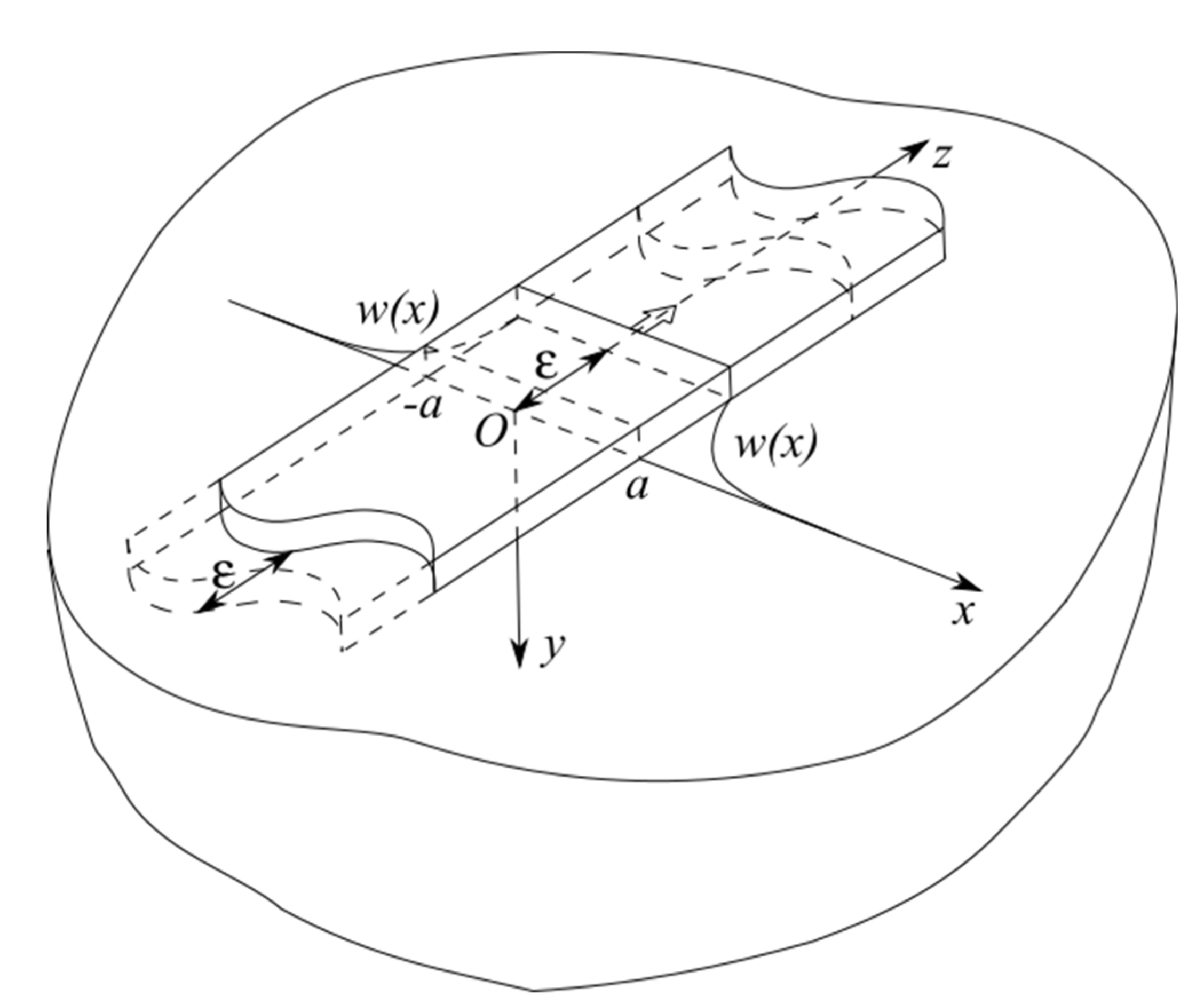
We consider the contact problem of elasticity theory about the shear of the elastic half-space surface ($y=0$) by a strip punch of width $2a$ ($\left|x\right|\le a$, $y=0$) with magnitude $\epsilon$ ($w(x,0)=\epsilon$, $\left|x\right|\le a$), where $w(x,y)$ is the shear displacement in the half-space $0\le y<\infty$ along the axis $z$. The scheme of the contact problem is presented on Figure 1.

The shear modulus of the functionally graded material in the half-space depends on the depth $y$ according to Equation (1). The contact stresses $\mathsf{\phi }(x)=-{\sigma }_{yz}(x,0)$ arising under the punch and other mechanical characteristics of the problem are to be determined. It is assumed that at infinity in half-space the displacements $w(x,y)$ and stresses ${\sigma }_{xz}(x,y)$, ${\sigma }_{yz}(x,y)$ vanish as $\sqrt{x^2+y^2}\to \infty$.

The exponential law of elastic modulus variation is chosen because of its wide occurrence in engineered systems and nature. Composition of bimaterial graded coatings often vary exponentially [38]. When studying the Oxford geological sediments [8], it was found that the shear modulus $\mathsf{\mu }(y)$ changes with depth by the exponential law with parameters ${\mathsf{\mu }}_0$ = 3.33 MPa, $2d$ = 0.0879 m⁻¹.

In the half-space under the pure shear deformation regime the conditions ${\sigma }_{xx}={\sigma }_{xy}={\sigma }_{yx}={\sigma }_{yy}={\sigma }_{zz}=0$ are fulfilled, where ${\sigma }_{xx}$, ${\sigma }_{yy}$ and ${\sigma }_{zz}$ are normal pressure components, and ${\sigma }_{yx}$, ${\sigma }_{xy}$ are tangential pressure components. Then the equations of the theory of elasticity in stresses [39] in the case of anti-plane deformation are as follows

$$\frac{\partial {\sigma }_{zx}}{\partial x}+\frac{\partial {\sigma }_{zy}}{\partial y}=0,$$

(2)

where ${\sigma }_{zx}$ and ${\sigma }_{zy}$, in case of functional inhomogeneity of elastic medium, are expressed through strains by formulae

$${\sigma }_{zx}=\mathsf{\mu }(y)\frac{\partial w}{\partial x}, {\sigma }_{zy}=\mathsf{\mu }(y)\frac{\partial w}{\partial y}.$$

(3)

By substituting Equation (3) into differential Equation (2) and then dividing it by $\mathsf{\mu }(y)\ne 0$, we obtain a differential equation in displacements

$$\frac{{\partial }^{2}w}{\partial y^2}+\frac{{\mathsf{\mu }}^{\prime }(y)}{\mathsf{\mu }(y)}\frac{\partial w}{\partial y}+\frac{{\partial }^{2}w}{\partial x^2}=0.$$

(4)

The differential Equation (4), with a factor $\mathsf{\mu }’(y)/\mathsf{\mu }(y)$ dependent on$y$, in case of $\mathsf{\mu }(y)={\mathsf{\mu }}_0{e}^{2dy}$ is transformed into a differential equation with constant coefficients

$$\frac{{\partial }^{2}w}{\partial y^2}+2d\frac{\partial w}{\partial y}+\frac{{\partial }^{2}w}{\partial x^2}=0.$$

(5)

Mixed boundary conditions of the formulated contact problem about the pure shear of surface of the functionally graded half-space by a strip punch at $y=0$ have the form

$$w(x,0)=\epsilon \hspace{1em}\left|x\right|\le a ,$$

(6)

$${\sigma }_{yz}(x,0)=\left\{\begin{array}{l}-\tilde{\mathsf{\phi }}(x)\hspace{1em}\left|x\right|\le a,\\ 0\hspace{1em}\hspace{1em}\hspace{1em}a<\left|x\right|<\infty \end{array}\right.,$$

(7)

where $\tilde{\mathsf{\phi }}(x)$ are the contact stresses under the punch to be determined.

At infinity $\sqrt{x^2+y^2}\to \infty$ displacement $w$ and its derivatives $\frac{\partial w}{\partial x}$, $\frac{\partial w}{\partial y}$ satisfy

$$\underset{\sqrt{x^2+y^2}\to \infty }{\lim }\left\{w,\frac{\partial w}{\partial x},\frac{\partial w}{\partial y}\right\}=0.$$

(8)

4. Integral Equation of the Problem

To construct the solution to the differential Equation (5) the Fourier integral transform is used:

$$w^F(\alpha ,y)={\displaystyle \underset{-\infty }{\overset{\infty }{\int }}w(x,y)e^{i\alpha x}\mathrm{d}x}, w(x,y)=\frac{1}{2\pi }{\displaystyle \underset{-\infty }{\overset{\infty }{\int }}{w}^F(\alpha ,y)e^{-i\alpha x}\mathrm{d}\alpha },$$

(9)

where the upper index $F$ means the Fourier transform of the function.

By means of the Fourier integral transform shown in Equation (9) and conditions at infinity shown in Equation (8) the differential Equation (5) is reduced to the solution of an ordinary differential equation with constant coefficients relative to the transform $w^F(\alpha ,y)$:

$$\frac{{\mathrm{d}}^2{w}^F}{\mathrm{d}{y}^2}+2d\frac{\mathrm{d}{w}^F}{\mathrm{d}y}-{\alpha }^2{w}^F=0.$$

(10)

The general solution to this equation, which vanishes at infinity ($y\to \infty$), has the form

$$w^F(\alpha ,y)=C(\alpha )e^{{\lambda }_{-}y}, {\lambda }_{-}=-d-\sqrt{d^2+{\alpha }^2}, d>0,$$

(11)

where $C(\alpha )$ is determined from the boundary condition of Equation (7) after application of the Fourier integral transform shown in Equation (9) and has the form

$$C(\alpha )=-\frac{{\tilde{\mathsf{\phi }}}^F(\alpha )}{{\mathsf{\mu }}_0{\lambda }_{-}^{}}.$$

The displacements $w(x,y)$ are determined from Equation (11) by means of the inverse Fourier transform of Equation (9) and have the form

$$w(x,y)=-{\left(2\pi {\mathsf{\mu }}_0\right)}^{-1}{\displaystyle \underset{-\infty }{\overset{\infty }{\int }}{\tilde{\mathsf{\phi }}}^F(\alpha )e^{{\lambda }_{-}y}{\lambda }_{-}^{-1}{e}^{-i\alpha x}\mathrm{d}\alpha },$$

(12)

where ${\tilde{\mathsf{\phi }}}^F(\alpha )$ is the transform of $\tilde{\mathsf{\phi }}(x)$.

Satisfying the mixed boundary conditions of Equations (6) and (7) and using Equation (12) we obtain the integral equation of the problem

$${\displaystyle \underset{-a}{\overset{a}{\int }}\tilde{\mathsf{\phi }}(\mathsf{\xi })k(\mathsf{\xi }-x)\mathrm{d}\mathsf{\xi }}=2\pi {\mathsf{\mu }}_0\epsilon , \left|x\right|\le a,$$

(13)

$$k(t)={\displaystyle \underset{-\infty }{\overset{\infty }{\int }}K(\alpha )e^{i\alpha t}\mathrm{d}\alpha }, K(\alpha )=-{\lambda }_{-}^{-1},$$

(14)

where ${\lambda }_{-}$ is from Equation (11).

It should be noted that at $d=0$ we obtain a classical integral equation for a homogeneous half-space with $\mathsf{\mu }(y)={\mathsf{\mu }}_0=const$.

By substituting $\alpha =d {\alpha }^{\prime }$, $\mathrm{d}\alpha =d \mathrm{d}{\alpha }^{\prime }$ into the internal integral and making internal $\mathsf{\xi }=a {\mathsf{\xi }}^{\prime }$, $\mathrm{d}\mathsf{\xi }=a \mathrm{d}{\mathsf{\xi }}^{\prime }$ and external $x=a x^{\prime }$ variables dimensionless, the integral Equations (13) and (14) are reduced to the integral equation in dimensionless form (primes omitted)

$${\displaystyle \underset{-1}{\overset{1}{\int }}\mathsf{\phi }(\mathsf{\xi })k\left(\frac{\mathsf{\xi }-x}{\lambda }\right)\mathrm{d}\mathsf{\xi }}=2\pi , \left|x\right|\le 1, \lambda =\frac{1}{da},$$

(15)

$$k(t)={\displaystyle \underset{-\infty }{\overset{\infty }{\int }}K(\alpha )e^{i\alpha t}\mathrm{d}\alpha }, K(\alpha )={\left(1+\sqrt{1+{\alpha }^2}\right)}^{-1},$$

(16)

which is an integral equation of the first kind of the Fourier convolution type with a difference kernel with respect to unknown dimensionless contact stresses $\mathsf{\phi }(x)=a{\epsilon }^{-1}{\mathsf{\mu }}_0^{-1}\tilde{\mathsf{\phi }}(x)$. The transform $K(\alpha )$ of the kernel $k(t)$ of Equation (16) in the integral Equation (15) is an even function, multi-valued in the complex plane $\alpha$ with algebraic branch points $\alpha =\pm i$ and expresses the following asymptotic properties:

$$K(\alpha )={\left|\alpha \right|}^{-1}+\mathrm{O}({\alpha }^{-2}) \mathrm{for} \left|\alpha \right|\to \infty ,$$

(17)

$$K(\alpha )=K(0)+\mathrm{O}({\alpha }^2) \mathrm{for} \left|\alpha \right|\to 0,$$

(18)

where $K(0)=0.5$. After calculating the integral in Equation (16), the kernel $k(t)$ looks like

$$k(t)=2e^t\left(K_0(t)-{\displaystyle \underset{t}{\overset{\infty }{\int }}\mathrm{d}\tau {\displaystyle \underset{\tau }{\overset{\infty }{\int }}{K}_0(\mathsf{\xi })\mathrm{d}\mathsf{\xi }}}\right),$$

(19)

where $K_0(t)$ is the McDonald’s function. At small $t$ for $k(t)$ the following behaviour takes place:

$$k(t)=-2\ln \left|t\right|+\mathrm{O}(1) \mathrm{at} t\to 0.$$

(20)

The properties listed for $k(t)$ allow us to conclude [40] that the solution to the integral Equation (15) exists and is unique in the class of functions $\mathsf{\phi }(x)=\omega (x){\left(1-x^2\right)}^{-1/2}$, where $\omega (x)\in C^1[-1,1]$.

For construction of effective analytical solutions of the integral Equations (15) and (16), we use asymptotic methods with respect to the dimensionless parameter $\lambda ={\left(da\right)}^{-1}$.

5. Effective Solution for Small λ

At small values of a dimensionless parameter $\lambda$ the solution to the integral Equations (15) and (16) are constructed as a Neumann series, the zeroth term of which is set by the ratio [40]

$$\mathsf{\phi }(x)={\mathsf{\phi }}_{+}\left((1+x){\mathsf{\lambda }}^{-1}\right)+{\mathsf{\phi }}_{-}\left((1-x){\mathsf{\lambda }}^{-1}\right)-{\mathsf{\phi }}_{\infty }(x{\mathsf{\lambda }}^{-1}).$$

(21)

Functions ${\mathsf{\phi }}_{\pm }(x)$ are determined from the Wiener-Hopf integral equation on a semi-axis [40,41], corresponding to Equation (15)

$${\displaystyle \underset{0}{\overset{\infty }{\int }}{\mathsf{\phi }}_{\pm }(\mathsf{\xi })k(\mathsf{\xi }-x)\mathrm{d}\mathsf{\xi }=\frac{2\pi }{\lambda }}, 0<x<\infty .$$

(22)

The function ${\mathsf{\phi }}_{\infty }(x)$ is determined from the integral Equation of the convolution type on an infinite interval, corresponding to Equation (15)

$${\displaystyle \underset{-\infty }{\overset{\infty }{\int }}{\mathsf{\phi }}_{\infty }(\mathsf{\xi })k(\mathsf{\xi }-x)\mathrm{d}\mathsf{\xi }=\frac{2\pi }{\lambda }},-\infty <x<\infty .$$

(23)

The solution to the integral Equation (23) is constructed using the generalized Fourier integral transform [42] and has the form

$${\mathsf{\phi }}_{\infty }(x)=\frac{1}{\lambda K(0)},-\infty <x<\infty .$$

(24)

The solution to the integral Equation (22) on a semi-axis is based on the Wiener-Hopf method [43]. In the first step of the method, the integral equation is extended to the whole axis. Thus, for ${\mathsf{\phi }}_{+}^{}(x)$ we have

$${\displaystyle \underset{0}{\overset{\infty }{\int }}{\mathsf{\phi }}_{+}(\mathsf{\xi })k(\mathsf{\xi }-x)\mathrm{d}\mathsf{\xi }=\left\{\begin{array}{ll}\frac{2\pi }{\lambda }\hfill & 0<x<\infty ,\hfill \\ \frac{2\pi }{\lambda }{v}_{-}(x)\hfill & -\infty <x<0,\hfill \end{array}\right.}$$

(25)

where $v_{-}(x)={\mathsf{\epsilon }}^{-1}{w}_{-}(x)$ are the dimensionless displacements of the free surface of the half space outside the contact area (to the left of the punch), which are given by the operator

$$v_{-}(x)={\displaystyle \underset{-\infty }{\overset{0}{\int }}{\mathsf{\phi }}_{+}(\mathsf{\xi })k(\mathsf{\xi }-x)\mathrm{d}\mathsf{\xi }},-\infty <x<0,$$

and $w_{-}(x)$ are the dimensional horizontal displacements of the free surface of the half space outside the contact area (to the left of the punch).

In the second step of the Wiener-Hopf method, the Fourier integral transform of Equation (9) is used to solve the integral Equation (25), by means of which the integral Equation (25) is reduced to a functional equation with respect to transforms ${\mathsf{\phi }}_{+}^F(\alpha )$, $v_{-}^F(\alpha )$ of unknown functions ${\mathsf{\phi }}_{+}^{}(x)$, $v_{-}^{}(x)$,

$${\mathsf{\phi }}_{+}^F(\alpha )K(\alpha )=\frac{1}{\lambda }\left(-\frac{1}{i\alpha }\right)+\frac{1}{\lambda }{v}_{-}^F(\alpha ), {\mathsf{\eta }}_{-}<\mathrm{Im}(\alpha )<{\mathsf{\eta }}_{+},$$

(26)

in which the unknown transforms

$${\mathsf{\phi }}_{+}^F(\alpha )={\displaystyle \underset{0}{\overset{\infty }{\int }}{\mathsf{\phi }}_{+}^{}(\mathsf{\xi })e^{i\alpha \mathsf{\xi }}\mathrm{d}\mathsf{\xi }}, v_{-}^F(\alpha )={\displaystyle \underset{-\infty }{\overset{0}{\int }}{v}_{-}^{}(\mathsf{\xi })e^{i\alpha \mathsf{\xi }}\mathrm{d}\mathsf{\xi }}$$

are regular in the upper ($\mathrm{Im}(\alpha )>{\mathsf{\eta }}_{-}$) and lower ($\mathrm{Im}(\alpha )<{\mathsf{\eta }}_{+}$) half-planes of the complex plane $\alpha$, respectively. Assuming that the factorization $K(\alpha )$ is known, i.e.,$K(\alpha )$ is represented as

$$K(\alpha )=K_{+}(\alpha )K_{-}(\alpha ),$$

(27)

where $K_{+}(\alpha )$ is regular in the upper ($\mathrm{Im}(\alpha )>{\mathsf{\eta }}_{-}$), and $K_{-}(\alpha )$ is regular in the lower ($\mathrm{Im}(\alpha )<{\mathsf{\eta }}_{+}$) half-plane, and after substitution of Equation (27) in Equation (26), the left and right parts of the resulting equation are divided on $K_{-}(\alpha )$. Let us introduce the representation

$$f(\alpha )=\frac{1}{i \alpha K_{-}(\alpha )}=f_{+}(\alpha )+f_{-}(\alpha ),$$

(28)

where $f_{+}(\alpha )$ is regular in the upper half-plane ($\mathrm{Im}(\alpha )>{\mathsf{\eta }}_{-}$) and $f_{-}(\alpha )$ in the lower half-plane ($\mathrm{Im}(\alpha )<{\mathsf{\eta }}_{+}$). Then Equation (26) can be written as

$${\mathsf{\phi }}_{+}^F(\alpha )K_{+}(\alpha )+\frac{1}{\lambda }{f}_{+}^{}(\alpha )=-\frac{1}{\lambda }{f}_{-}^{}(\alpha )+\frac{1}{\lambda }\frac{v_{-}^F(\alpha )}{K_{-}(\alpha )}, {\mathsf{\eta }}_{-}<\mathrm{Im}(\alpha )<{\mathsf{\eta }}_{+},$$

(29)

which holds in the strip ${\mathsf{\eta }}_{-}<\mathrm{Im}(\alpha )<{\mathsf{\eta }}_{+}$, the left and right part of which are continuations of some complex variable function $F(\alpha )$ in the upper ($\mathrm{Im}(\alpha )>{\mathsf{\eta }}_{-}$) and lower ($\mathrm{Im}(\alpha )<{\mathsf{\eta }}_{+}$) half-planes, correspondingly. Since the left and right parts vanish at infinity ($\left|\alpha \right|\to \infty$), the function $F(\alpha )=0$ in the complex plane $\alpha =\mathsf{\xi }+i\mathsf{\eta }$. Then two equations follow from Equation (29):

$${\mathsf{\phi }}_{+}^F(\alpha )=-\frac{1}{\lambda }\frac{f_{+}^{}(\alpha )}{K_{+}(\alpha )},$$

(30)

$$v_{-}^F(\alpha )=K_{-}(\alpha )f_{-}^{}(\alpha ),$$

(31)

$$f_{+}^{}(\alpha )=\frac{1}{K_{-}(0) i\alpha }, f_{-}^{}(\alpha )=\frac{K_{-}(0)-K_{-}(\alpha )}{K_{-}(0) i\alpha K_{-}(\alpha )},$$

which are used to determine the unknown transforms. Inverting the Fourier transform in Equations (30) and (31) with the help of Equation (9) we obtain the solution to integral Equation (25):

$${\mathsf{\phi }}_{+}(x)=-\frac{1}{\lambda K_{-}(0)}\frac{1}{2\mathsf{\pi }}{\displaystyle \underset{-\infty +ic}{\overset{\infty +ic}{\int }}\frac{e^{-i\alpha x}}{i\alpha K_{+}(\alpha )}\mathrm{d}\alpha }, x>0,$$

(32)

and determine $v_{-}(x)$ as

$$v_{-}(x)=\frac{1}{2\mathsf{\pi }}{\displaystyle \underset{-\infty +id}{\overset{\infty +id}{\int }}\left(\frac{1}{i\alpha }-\frac{1}{K_{-}(0)}\frac{K_{-}(\alpha )}{i\alpha }\right)e^{-i\alpha x}\mathrm{d}\alpha }, x<0,$$

(33)

where ${\mathsf{\eta }}_{-}<c<d<{\mathsf{\eta }}_{+}$, and ${\mathsf{\eta }}_{\pm }$ is taken as $\pm 1$ based on the properties of $K(\alpha )$ from Equation (16).

The integral representations for ${\mathsf{\phi }}_{-}^{}(x)$ and $v_{+}(x)$ completely coincide with Equations (32) and (33), respectively, where $v_{+}(x)={\epsilon }^{-1}{w}_{+}(x)$, $v_{+}(x)$ and $w_{+}(x)$ are the dimensionless and dimensional (correspondingly) displacements of the free surface of the half-space outside the contact area (to the right of the punch).

In order to calculate integrals in Equations (32) and (33) with $K_{\pm }(\alpha )$, it is necessary to perform the factorization of kernel transform $K(\alpha )$ of Equation (27). The exact factorization $K(\alpha )$ of Equation (16) was previously given in [43] but it is not very effective for obtaining a foreseeable solution. To get the effective solution, we use the $K(\alpha )$ approximation that can be factorized by elementary means.

As the simplest approximations of $K(\alpha )$ satisfying the properties of Equations (17) and (18) and having no zeros and poles in the strip ${\mathsf{\eta }}_{-}<\mathrm{Im}(\alpha )<{\mathsf{\eta }}_{+}$, let us take the following functions:

$$(\mathrm{a}) K(\alpha )=\frac{1}{\sqrt{A^2+{\alpha }^2}}, A=\frac{1}{K(0)},$$

(34)

$$(\mathrm{b}) K(\alpha )=\frac{1}{\sqrt{A^2+{\alpha }^2}}\frac{B^2+{\alpha }^2}{C^2+{\alpha }^2}, \frac{1}{A}\frac{B^2}{C^2}=K(0), \mathrm{and}$$

(35)

$$(\mathrm{c}) K(\alpha )=\frac{\sqrt{A^2+{\alpha }^2}}{D^2+{\alpha }^2}\frac{B^2+{\alpha }^2}{C^2+{\alpha }^2}, \frac{A}{D^2}\frac{B^2}{C^2}=K(0).$$

(36)

The error of such $K(\alpha )$ approximations in the strip $\left|\mathrm{Im}(\alpha )\right|<\inf \left({\mathsf{\eta }}_{-},{\mathsf{\eta }}_{+}\right)$ along the real axis ($\mathrm{Im}(\alpha )=0$) does not exceed (a) 12%, (b) 4%, (c) 2% for the Equations (34)–(36), respectively. The values of the parameters in Equations (34)–(36) are listed in

Table 1. The values of the approximation parameters.

$\mathit{K}(\mathit{\alpha })$	A	B	C	D
(34)	2	–	–	–
(35)	1.5344	6.0332	6.8881	–
(36)	3.5897	3.9419	1.9665	5.3710

.

The factorization of $K(\alpha )$ in the form of Equation (27) using the approximations given by Equations (34)–(36) is achieved by elementary means:

$$(\mathrm{a}) K_{\pm }(\alpha )=\frac{1}{\sqrt{A\mp i\alpha }},$$

(37)

$$(\mathrm{b}) K_{\pm }(\alpha )=\frac{1}{\sqrt{A\mp i\alpha }}\frac{B\mp i\alpha }{C\mp i\alpha },$$

(38)

$$(\mathrm{c}) K_{\pm }(\alpha )=\frac{\sqrt{A\mp i\alpha }}{D\mp i\alpha }\frac{B\mp i\alpha }{C\mp i\alpha },$$

(39)

where $K_{+}(\alpha )$ is regular in the upper half-plane ($\mathrm{Im}(\alpha )>{\mathsf{\eta }}_{-}$), and $K_{-}(\alpha )$ is regular in the lower half-plane ($\mathrm{Im}(\alpha )<{\mathsf{\eta }}_{+}$), and ${\mathsf{\eta }}_{\pm }=\inf \left(A,B,C,D\right)$ for each of the cases (a), (b) and (c). Substituting $K_{\pm }(\alpha )$ from Equations (37)–(39) and calculating the integral in Equation (32), the following solutions of the integral Equation (22) are obtained

$$(\mathrm{a}) {\mathsf{\phi }}_{\pm }(x)=\frac{1}{\lambda K_{-}(0)}\mathsf{\Phi }\left(x,A,0\right), x>0,$$

(40)

$$(\mathrm{b}) {\mathsf{\phi }}_{\pm }(x)=\frac{1}{\lambda K_{-}(0)}\left(\frac{C}{B}\mathsf{\Phi }\left(x,A,0\right)+\frac{B-C}{B}\mathsf{\Phi }\left(x,A,B\right)\right), x>0,$$

(41)

$$\begin{gathered} (\mathrm{c}) {\mathsf{\phi }}_{\pm }(x)=\frac{1}{\lambda K_{-}(0)}\left(\frac{DC}{AB}\mathsf{\Phi }\left(x,A,0\right)+\frac{\left(D-A\right)\left(C-A\right)}{A\left(A-B\right)}\frac{1}{\sqrt{\mathsf{\pi }x}}{e}^{-Ax}+\right. \\ \left.+\frac{\left(D-B\right)\left(C-B\right)}{B\left(B-A\right)}\mathsf{\Phi }\left(x,A,B\right)\right), x>0, \end{gathered}$$

(42)

where $\mathsf{\Phi }\left(x,A,B\right)=\frac{1}{\sqrt{\pi x}}{e}^{-Ax}+\sqrt{A-B}{e}^{-Bx}\mathrm{erf}\left(\sqrt{\left(A-B\right)x}\right)$, and $\mathrm{erf}\left(x\right)$ is the probability integral [44].

Calculating the square in Equation (33), after the substitution of$K_{-}(\alpha )$ from Equations (37)–(39) we obtain displacements outside the punch:

$$(\mathrm{a}) v_{\mp }(x)=\mathrm{erfc}\left(\sqrt{A(-x)}\right), x<0,$$

(43)

$$(\mathrm{b}) v_{\mp }(x)=1-\frac{1}{\sqrt{A}}\mathsf{\Phi }\left(-x,A,0\right)+\frac{\sqrt{A}C}{B(C-A)}\cdot \left(\frac{B-A}{A}\frac{e^{-A(-x)}}{\sqrt{\pi (-x)}}-\frac{B-C}{C}\mathsf{\Phi }\left(-x,A,C\right)\right), x<0,$$

(44)

$$(\mathrm{c}) v_{\mp }(x)=1-\frac{1}{\sqrt{A}}\mathsf{\Phi }\left(-x,A,0\right)-\frac{DC}{\sqrt{A}B(D-C)}\cdot \left(\frac{B-D}{D}\mathsf{\Phi }\left(-x,A,D\right)-\frac{B-C}{C}\mathsf{\Phi }\left(-x,A,C\right)\right), x<0,$$

(45)

where $\mathrm{erfc}\left(x\right)=1-\mathrm{erf}\left(x\right)$ [44], and $\mathsf{\Phi }\left(x,A,B\right)$ is given after Equation (42).

Substituting${\mathsf{\phi }}_{\pm }(x)$ from Equations (34)–(36) and ${\mathsf{\phi }}_{\infty }(x)$ from Equations (24) to (21), we obtain the solution of the integral equation of the problem shown in Equation (15). After returning in Equations (43)–(45) to the initial set of variables, the functions $v_{\mp }\left((1\pm x){\lambda }^{-1}\right)$ give horizontal displacements of the stress-free surface of the half-space outside the contact area at $1\pm x<0$.

The punch shear force $\tilde{T}$, which is an integral characteristic of the problem, is determined by the integration of the obtained solution over the interval $[-a,a]$

$$\tilde{T}={\displaystyle \underset{-a}{\overset{a}{\int }}\tilde{\mathsf{\phi }}\left(x\right)\mathrm{d}x}=a{\displaystyle \underset{-1}{\overset{1}{\int }}\tilde{\mathsf{\phi }}\left(x\right)\mathrm{d}x}=\epsilon {\mathsf{\mu }}_{0}T,$$

(46)

where

$$T={\displaystyle \underset{-1}{\overset{1}{\int }}\mathsf{\phi }\left(x\right)\mathrm{d}x}$$

(47)

is a dimensionless shear force. Taking $\mathsf{\phi }(x)$ in the form of a superposition Equation (21) and integrating over the interval $[-1, 1]$, we obtain the dimensionless shear force $T$ in the form

$$T=T_{+}+T_{-}-T_{\infty }, T_{\pm }={\displaystyle \underset{-1}{\overset{1}{\int }}{\mathsf{\phi }}_{\pm }\left(\frac{1\pm x}{\lambda }\right)\mathrm{d}x}, T_{\infty }={\displaystyle \underset{-1}{\overset{1}{\int }}{\mathsf{\phi }}_{\infty }\left(\frac{x}{\lambda }\right)\mathrm{d}x}.$$

(48)

The use of an asymptotic solution to the integral Equation (15) in multiplicative form [40]

$$\mathsf{\phi }(x)={\mathsf{\phi }}_{+}\left((1+x){\lambda }^{-1}\right) {\mathsf{\phi }}_{-}\left((1-x){\lambda }^{-1}\right) {\mathsf{\phi }}_{\infty }^{-1}(x{\lambda }^{-1}),$$

(49)

where ${\mathsf{\phi }}_{\pm }\left((1\pm x){\lambda }^{-1}\right)$ from Equations (40)–(42), and ${\mathsf{\phi }}_{\infty }^{}(x{\lambda }^{-1})$ from Equation (24), allows for more convenient formulae for $T$ to analyse all considered approximations of $K(\alpha )$ listed in Equations (34)–(36):

$$(\mathrm{a}) T=1+A\gamma ,$$

(50)

$$\left(\mathrm{b}\right) T={\left(\frac{C}{B}\right)}^2\left(1+2\frac{A}{C}\frac{B-C}{B}+A\gamma \right)+{\left(\frac{C-B}{B}\right)}^2\left(1+2\frac{C}{B}\frac{A-B}{C-B}+(A-B)\gamma \right)e^{-\gamma B},$$

(51)

$$\left(\mathrm{c}\right) T=\kappa \left(A\right)+{\kappa }_{*}\left(0\right)\left(z_{-}\left(0\right)+A\gamma \right)+\kappa \left(B\right)\left(z_{+}\left(B\right)+\left(A-B\right) \gamma \right),$$

(52)

where

$$\gamma =2 {\lambda }^{-1}=2ad,$$

$$\kappa \left(t\right)={\left(\frac{\left(D-t\right)\left(C-t\right)}{t\left(A-B\right)}\right)}^2{e}^{-\gamma t}, {\kappa }_{*}\left(t\right)={\left(\frac{\left(D-t\right)\left(C-t\right)}{\left(A-t\right)\left(B-t\right)}\right)}^2{e}^{-\gamma t},$$

$$z_{\pm }\left(t\right)=-1+2\left(\frac{B}{D-t}+\frac{B}{C-t}\pm 1\right)\frac{A-t}{B}.$$

Equations (50)–(52) have the same order of accuracy for small $\lambda$ as in Equation (46).

6. Effective Solution for Large λ

When constructing the solution to the integral equation of the problem listed in Equations (15) and (16) in the case of large values of $\lambda$, it is necessary to take into account the fact that $K(\alpha )$ can be represented by a series

$$K(\alpha )={\displaystyle \sum _{k=0}^N{c}_k{\left|\alpha \right|}^{-k-1}+O\left({\left|\alpha \right|}^{-N-2}\right)} \mathrm{having} 0<m<\left|\alpha \right|<\infty ,$$

(53)

in which $c_k$ at $k=0, 1, 2 ,\dots ,N$ and for $N=4$ have the following values:

$$c_0=1, c_1=-1, c_2=\frac{1}{2}, c_3=0, c_4=-\frac{1}{8}.$$

With the help of series representation by Equation (53) and the asymptotic property shown in Equation (17), it is not difficult to obtain the decomposition of $k(t)$ in the form of the following series [45]

$$\frac{1}{2}k(t)=-\ln \left|t\right|+a_{20}\left|t\right|+a_{11}{t}^2\ln \left|t\right|+a_{21}{\left|t\right|}^3+a_{31}{t}^2+O\left(t^4\ln \left|t\right|\right) \mathrm{at} t\to 0,$$

(54)

where

$$a_{20}=-\frac{\pi }{2}{c}_1, a_{11}=\frac{1}{2}{c}_2, a_{21}=\frac{1}{12}\pi c_3, \mathrm{and}{a}_{31}=-\frac{3}{4}{c}_2+\frac{1}{2}{\displaystyle \underset{0}{\overset{\infty }{\int }}\left[{\alpha }^2-{\alpha }^{3}K(\alpha )+c_1\alpha +c_2(1-e^{-\alpha })\right] {\alpha }^{-1}d\alpha }.$$

(55)

After substitution of Equation (54) into Equation (15) and the differentiation by an external variable $x$, a singular integral equation is obtained with respect to $\mathsf{\phi }(x)$. Inverting the singular integral equation, an equivalent integral equation of the second kind is formed [45]. The solution to the latter is constructed by the successive approximations method in the form of a double functional series

$$\mathsf{\phi }(x)=\frac{T}{a\sqrt{1-x^2}}{\displaystyle \sum _{m=0}^{\infty } {\displaystyle \sum _{n=0}^{\infty }{\omega }_{mn}(x){\lambda }^{-m}{\ln }^n\lambda }}, n\le \left[\frac{m}{2}\right],$$

(56)

with the following expressions for functions ${\omega }_{mn}(x)$:

$$\begin{gathered} {\omega }_{00}(x)={\pi }^{-1}, {\omega }_{10}(x)=4{\pi }^{-3}{a}_{20}{S}_1(x), {\omega }_{11}(x)=0, {\omega }_{01}(x)=0, \\ {\omega }_{20}(x)={\pi }^{-1}\left(a_{131}\left(1-2x^2\right)+32{\pi }^{-4}{a}_{20}^2\left(S_2(x)-0.1508\right)\right), \\ {\omega }_{21}(x)=-{\pi }^{-1}{a}_{11}\left(1-2x^2\right), {\omega }_{31}(x)=-2{\pi }^{-3}{a}_{11}{a}_{20}{S}_4(x), \mathrm{and} \\ {\omega }_{30}(x)={\pi }^{-3}\left(\frac{8}{3}{a}_{21}+{\displaystyle \sum _{k=0}^4{b}_{1k}(x)}{S}_{1+k}(x)\right), \end{gathered}$$

(57)

where

$$\begin{gathered} b_{12}=\frac{8}{9}{a}_{11}{a}_{20}, b_{10}(x)=6a_{21}\left(1+2x^2\right)-19.3024{\pi }^{-4}{a}_{20}^3, b_{11}=0, \\ {b}_{13}=9a_{21}+2a_{131}{a}_{20}, a_{131}=a_{11}\left(\frac{3}{2}-\ln 2\right)+a_{31}, b_{14}(x)=64{\pi }^{-4}{a}_{20}^3, \\ {S}_1(x)=\left(1-2x^2\right)+2\sqrt{1-x^2}{\displaystyle \sum _{k=1}^{\infty }{c}_{2k+1}(x)}, c_n(x)=n^{-2}\sin (n\arccos x), \\ {S}_2(x)=\left(0.4356+0.1321x^2\right)\left(1-x^2\right)+0.2494 x l(x), \\ {S}_3(x)=-\left(1-2x^2\right)+144\sqrt{1-x^2}{\displaystyle \sum _{k=1}^{\infty }{\left(2k-1\right)}^{-2}{\left(2k+3\right)}^{-2}{c}_{2k+1}(x)}, \\ {S}_4(x)=\frac{1}{3}+\left(1-2x^2\right)+x l(x), l(x)=\left(1-x^2\right)\ln \frac{1-x}{1+x}, \\ {S}_5(x)=r_1(x)+x l(x) r_2(x)-0.04156 l^2(x)+0.3026 S_1(x), \mathrm{and} \\ {r}_1(x)=0.3547-0.8463 x^2+0.3442 x^4, r_2(x)=0.1180+0.03305 x^2. \end{gathered}$$

The dimensionless shear force (47) then takes the form

$$\begin{array}{l}T=\pi \left((\ln (2\lambda )(1-a_{11}{\lambda }^{-2}+0.1801a_{11}{a}_{20}{\lambda }^{-3})+a_{31}\right.+0.8106a_{20}{\lambda }^{-1}+\left(a_{31}+a_{11}-0.03287a_{20}{}^2\right) {\lambda }^{-2}+\\ {\left.+\left(1.442a_{21}-0.2702a_{11}{a}_{20}-0.1807a_{31}{a}_{20}-0.02450a_{20}{}^3\right) {\lambda }^{-3}+O\left({\lambda }^{-4}\right)\right)}^{-1}\end{array}$$

(58)

7. Analysis and Application of the Obtained Solutions

The obtained asymptotic solutions by the parameter $\lambda ={\left(da\right)}^{-1}$ of the exponentially functionally graded material shear problem cover the entire range of the parameter $\lambda \in \left(0, \infty \right)$.

Table 2. Relative contact stresses $a{T}^{-1}\mathsf{\phi }(0)$ for $a=1$ m and different $\lambda$.

$a{T}^{-1}\mathsf{\phi }(0)$	λ = 1.0	λ = 1.5	λ = 2.0
(40), (24), (50)	0.4068	0.3828	0.3668
(41), (24), (51)	0.3988	0.3803	0.3690
(42), (24), (52)	0.3965	0.3798	0.3701
(56), (57), (58)	0.4299	0.3909	0.3749

shows the numerical values of the relative contact stresses $a{T}^{-1}\mathsf{\phi }(0)$ calculated by Equations (21), (24), (40)–(42), and (50)–(52) in the case of small $\lambda$ ($\lambda \le 1$), and by Equations (56)–(58) in the case of large $\lambda$ ($\lambda \ge 2$), for $\lambda \in 1.0, 1.5, 2.0$ and $a=1$ m.

The analysis of values of the relative contact stresses shows that the solutions obtained for small and large values of $\lambda$ coincide on the interval $\lambda \in (1 , 2)$.

8. Determination of Shear Modulus Parameters

Previously, it was noted that researchers are increasingly focused on the development of methods for determining the parameters of elastic moduli of functionally graded materials [22,23,24,25,26,27], based on numerical solutions to contact problems on indentation. The analytical solutions of the problem obtained in the previous paragraphs allow us to analyse the correlation between mechanical parameters of the problem.

Table 3. Relative contact stresses $a{T}^{-1}\mathsf{\phi }(0)$ for $a=1$ and different values of shear modulus parameter $d$.

$\lambda$	$d$ (m−1)	$a{T}^{-1}\mathsf{\phi }(0)$	$\frac{T^{-1}\mathsf{\phi }(0)}{T_0{}^{-1}{\mathsf{\phi }}_0(0)}$	$h$ (m)
0.1	10	0.4878	1.53	0.0005
0.2	5	0.4762	1.50	0.0010
1.0	1.0	0.4068	1.28	0.0053
5	0.2	0.3450	1.08	0.0263
10	0.1	0.3329	1.05	0.0527
103	10−3	0.3185	1.00	5.27

shows the values of the relative stresses $a{T}^{-1}\mathsf{\phi }(0)$ in the centre of the punch, where $x=0$ at $a=1$ m for the different values of the parameter $d$. At small $d$, for example at $d=0.001$ ($\lambda =1000$), the value of the relative stresses $a{T}^{-1}\mathsf{\phi }(0)$ coincides with the value of the relative contact stress $a{T}_0{}^{-1}{\mathsf{\phi }}_0(0)$ at $x=0$ in the classical solution to the homogeneous half-space shear problem [45]

$$a{T}_0{}^{-1}{\mathsf{\phi }}_0(x)={\left(\pi \sqrt{1-x^2}\right)}^{-1},$$

that for $x=0$ is $a{T}_0{}^{-1}{\mathsf{\phi }}_0(0)={\pi }^{-1}=0.3183$. At $d=10$ ($\lambda =0.1$) the value $a{T}^{-1}\mathsf{\phi }(0)=0.4878$, i.e., $1.53$ times the value $a{T}^{-1}\mathsf{\phi }(0)$ at $d=0.001$ ($\lambda =1000$), which also coincides with the classical solution. It follows that the parameter $d$ of the shear modulus $\mathsf{\mu }(y)$ as in Equation (1) affects the contact stresses. The meaning of the parameter h in Table 3 is explained in Section 9.

The data in Table 3 can be used to solve the problem of determining the shear modulus parameter $d$ by the values of the relative contact stresses $a{T}^{-1}\mathsf{\phi }(0)$ in the centre of the contact area in the following way.

Firstly, the parameter $d$ ($0<d<\infty$) of the functionally graded half-space shear modulus is determined from the solution to the transcendental equation with respect to $d$ (at $a=1$ m)

$${\tilde{T}}^{-1}\tilde{\mathsf{\phi }}(0)=T^{-1}\mathsf{\phi }(0)=\left\{\begin{array}{}\mathrm{(59)}& {\displaystyle \sum _{m=0}^{\infty } {\displaystyle \sum _{n=0}^{\infty }{(-1)}^n{\omega }_{mn}(0)d^m{\ln }^n\left(d\right)}} ,\hspace{1em}\hspace{1em}0<d<1 ,\mathrm{(60)}& {\mathsf{\phi }}_{+}(d)+{\mathsf{\phi }}_{-}(d)-{\mathsf{\phi }}_{\infty }(0) ,\hspace{1em}\hspace{1em}1<d<\infty , \end{array}\right.$$

where ${\omega }_{mn}(x)$ are from Equation (57), ${\mathsf{\phi }}_{\pm }(x)$ are from Equations (40)–(42), and ${\mathsf{\phi }}_{\infty }(x)$ is from Equation (24). In Equation (59) $T$ is taken from Equation (58), and in Equation (60) $T$ is taken from Equation (24). $\tilde{T}$ and $\tilde{\mathsf{\phi }}(0)$ are the force and value of contact stresses in the middle of the punch, determined experimentally or by some other means.

Secondly, to determine the shear ${\mathsf{\mu }}_0$ modulus parameter, which coincides with the value of the shear modulus on the half-space surface (at $y=0$), the static condition of Equation (46) is used:

$${\mathsf{\mu }}_0=\frac{\tilde{T}}{\epsilon T},$$

(61)

where $\tilde{T}$ is a shear force determined from experiment. The value $T$ of Equation (47) is determined for $0<d<1$ and $1<d<\infty$ from Equations (59) and (60), respectively.

Table 4. Relative stresses $a{T}^{-1}\mathsf{\phi }(x)$ at different values of the coordinate x.

$\lambda$	$d$ (m−1)	$a{T}^{-1}\mathsf{\phi }(0.00)$	$a{T}^{-1}\mathsf{\phi }(0.25)$	$a{T}^{-1}\mathsf{\phi }(0.50)$	$a{T}^{-1}\mathsf{\phi }(0.75)$
0.1	10	0.4854	0.4854	0.4854	0.4854
0.2	5	0.4715	0.4715	0.4716	0.4747
1	1	0.3965	0.4016	0.4217	0.4823
5	0.2	0.3451	0.3535	0.3849	0.4794
10	0.1	0.3330	0.3423	0.3771	0.4803
103	10−3	0.3185	0.3289	0.3677	0.4812

shows the values of the relative stresses $a{T}^{-1}\mathsf{\phi }(x)$ at points $x=0.00, 0.25, 0.50, 0.75$ for the same values of parameters $\lambda$ and $d$ as in Table 3 (at $a=1$m).

The abovementioned example of determining the parameter $d$ of the depth-varying shear modulus $\mathsf{\mu }(y)$ as defined in Equation (1) by values of contact stresses $a{T}^{-1}\mathsf{\phi }(x)$ is difficult to implement in practice due to the fact that contact stresses are not directly measured (or almost cannot be measured) and at best are determined indirectly or approximated. In the latter case, the approximate value of contact stresses $\tilde{\mathsf{\phi }}(0)$ is often taken as the ratio of an experimentally determined shear force $\tilde{T}$ to the contact length $2a$, i.e., $\tilde{\mathsf{\phi }}(0)=0.5 \tilde{T}{a}^{-1}$. The indirect and approximated methods for determining contact stresses lead to additional errors in determining the shear modulus parameters. In this regard, we also propose another method for determination of the parameter $d$ of shear modulus $\mathsf{\mu }(y)$ using an experimentally and theoretically determined value of displacement $w(x)$ of the free material surface outside the contact area.

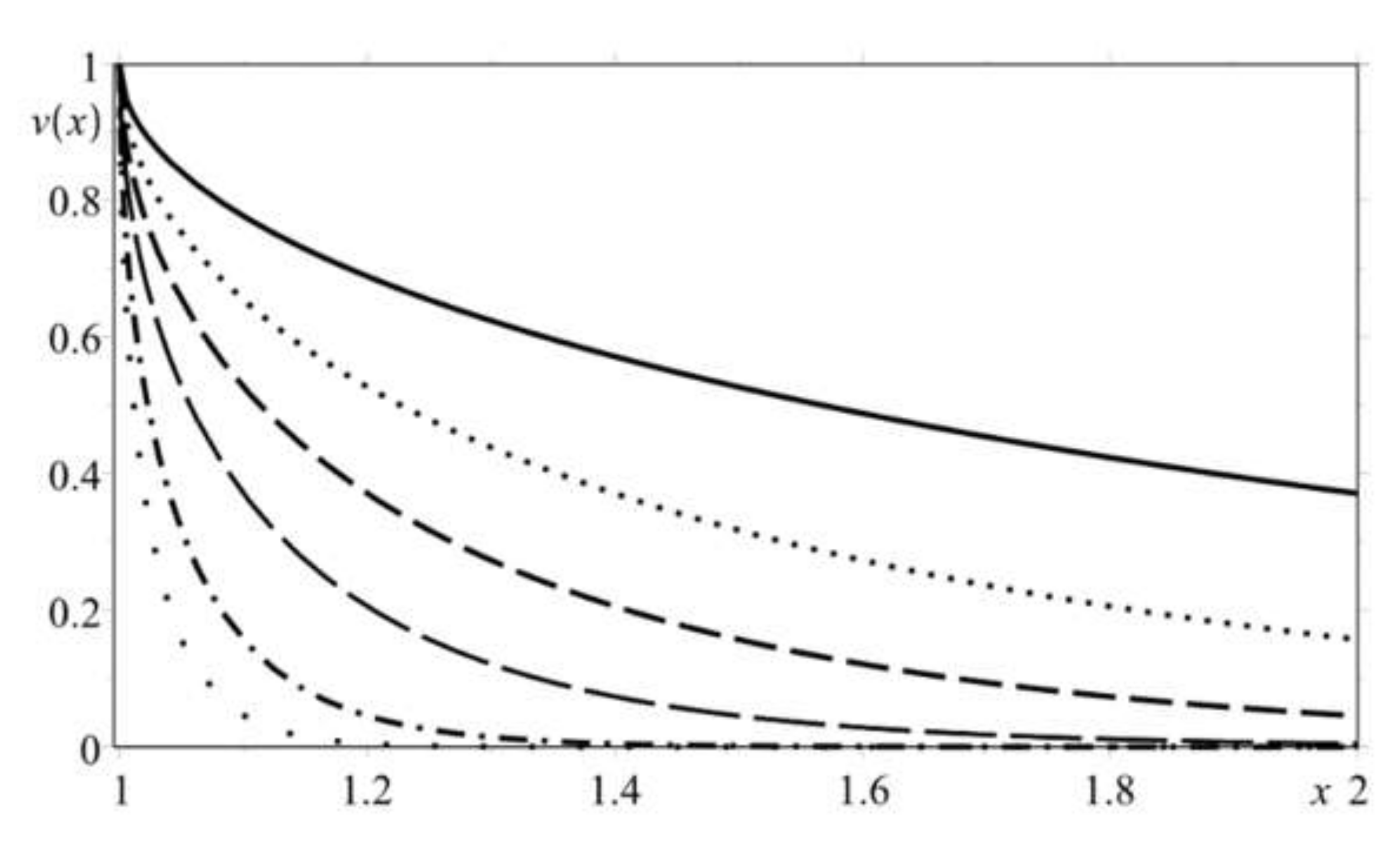
Figure 2 shows plots of dimensionless free surface displacement $v(x)$ to the right of the punch for $d=5, 2, 1, 0.5, 0.2, 0.1$ (at $a=1$).

Table 5. Dimensionless displacements $v(x)$ of the free surface.

$\lambda$	$d$ (m−1)	$v\left(1.01\right)$	$v\left(1.10\right)$	$v\left(1.20\right)$	$v\left(1.30\right)$	$v\left(1.40\right)$	$v\left(1.50\right)$
0.1	10	0.5271	0.0455	0.0047	0.0005	0.0001	0.0000
0.2	5	0.6547	0.1573	0.0455	0.0143	0.0047	0.0016
0.5	2	0.7773	0.3711	0.2059	0.1213	0.0736	0.0455
1	1	0.8415	0.5271	0.3711	0.2733	0.2059	0.1573
2	0.5	0.8875	0.6547	0.5271	0.4386	0.3711	0.3173
5	0.2	0.9287	0.7773	0.6892	0.6242	0.5716	0.5271

shows the values of the dimensionless displacements $v(x)$ ($v(x)={\epsilon }^{-1}w(x)$) outside the contact area for $1<\left|x\right|<\infty$ at $x=1.01, 1.1, 1.2, 1.3, 1.4, 1.5$, calculated for the values $\lambda$ and $d$ in Table 5 (at $a=1$). Displacements $w(x)$ at large $\lambda$ and $1<\left|x\right|<\infty$ are calculated by the formula

$$w(x)=\frac{\epsilon }{\pi }{\displaystyle \underset{-1}{\overset{1}{\int }}\mathsf{\phi }(\mathsf{\xi })k\left(\frac{\mathsf{\xi }-x}{\lambda }\right)\mathrm{d}\mathsf{\xi }}, 1<\left|x\right|<\infty ,$$

(62)

where $\mathsf{\phi }(x)$ is defined by the Equation (56), and $k\left(t\right)$ by Equation (16). At small $\lambda$ the displacements of the free surface $w(x)$ are calculated using the equation

$$w(x)=\epsilon v_{+}\left(\frac{1+x}{\lambda }\right)H(-1-x)+\epsilon v_{-}\left(\frac{1-x}{\lambda }\right)H(-1+x), 1<\left|x\right|<\infty ,$$

(63)

where $v_{\mp }(x)$ are defined by Equations (43)–(45); $H(x)$ is the Heaviside function.

The parameter $d$ ($0<d<\infty$) of the shear modulus $\mathsf{\mu }(y)$ from Equation (1) is determined from the solution to the following transcendental equation for $\left|x\right|\in (1,\infty )$ (at $a=1$):

$$w(x)=\left\{\begin{array}{}\mathrm{(64)}& \frac{\epsilon }{\pi }{\displaystyle \underset{-1}{\overset{1}{\int }}\mathsf{\phi }(\mathsf{\xi })k\left(d\left(\mathsf{\xi }-x\right)\right)\mathrm{d}\mathsf{\xi }} ,\hspace{1em}\hspace{1em}0<d<1 ,\mathrm{(65)}& \epsilon \left(v_{+}\left(d\left(1+x\right)\right)H(-1-x)+v_{-}\left(d\left(1-x\right)\right)H(-1+x)\right) ,\hspace{1em}\hspace{1em}1<d<\infty ,\end{array}\right.$$

The second parameter of the shear modulus ${\mathsf{\mu }}_0$ is determined, as in the previous case, from the static condition by Equation (61) through an experimentally determined punch shear force $\tilde{T}$.

Here we should also pay attention to the possibility of the parameter $d$ estimation through the slope of the displacements curve $w(x)$ outside the contact area (at $1<\left|x\right|<\infty$), which is numerically equal to the value of the derivative $w^{\prime }(x)$ for $1<\left|x\right|<\infty$ and which can be determined by experimental means. To determine $w^{\prime }(x)$, it is sufficient to differentiate the Equations (64) and (65), that is

$$w^{\prime }(x)=\left\{\begin{array}{}\mathrm{(66)}& \frac{\epsilon }{\pi }\left(2{\displaystyle \underset{-1}{\overset{1}{\int }}\frac{\mathsf{\phi }(\mathsf{\xi })}{\mathsf{\xi }-x}\mathrm{d}\mathsf{\xi }}-2d{\displaystyle \underset{-1}{\overset{1}{\int }}\mathsf{\phi }(\mathsf{\xi })k_{*}\left(d\left(\mathsf{\xi }-x\right)\right)\mathrm{d}\mathsf{\xi }}\right) ,\hspace{1em}\hspace{1em}0<d<1 ,\mathrm{(67)}& \epsilon d \left({v^{\prime }}_{+}\left(d\left(1+x\right)\right)H(-1-x)+{v^{\prime }}_{-}\left(d\left(1-x\right)\right)H(-1+x)\right) ,\hspace{1em}\hspace{1em}1<d<\infty ,\end{array}\right.$$

in which $\mathsf{\phi }(x)$ is from Equation (56), and the function $k_{*}\left(t\right)$ is given by the equation

$$k_{*}(t)={\displaystyle \underset{-\infty }{\overset{\infty }{\int }}{K}_{*}(\alpha )\sin (d(\mathsf{\xi }-x)\alpha )\mathrm{d}\alpha }, K^{*}(\alpha )=\mathrm{sgn}(\alpha ){\left(1+\left|\alpha \right|+\sqrt{1+{\alpha }^2}\right)}^{-1},$$

(68)

and $v_{\mp }(x)$ is defined in Equations (43)–(45). As before, the second parameter ${\mathsf{\mu }}_0$ of the shear modulus $\mathsf{\mu }(y)$ from Equation (1) is determined by the Equation (61).

For practical implementation of this method, one needs to measure displacements at several points of the free surface, for example, by using laser triangulation measurement [46] or interferometry [47].

Other additional conditions can be proposed from which the parameters of the exponential shear modulus as in Equation (1) of the functionally graded material can be determined.

Thus, the analytical solutions of the contact problem obtained here allowed us to effectively determine the parameters $d$ and ${\mathsf{\mu }}_0$ of the shear modulus $\mathsf{\mu }(y)$ of Equation (1) of a functionally graded half space.

9. “Approximate Homogeneous” Area

The fifth column of Table 3 indicates the depth coordinate $h$ in the functionally graded half-space for which the values of the shear modulus $\mathsf{\mu }(y)$ on the segment $\left[0,h\right]$ and the values of the shear modulus ${\mathsf{\mu }}_0$ on the half-space surface differ by no more than 1%. This means that using the shear modulus parameter$d$ in a half-space, with an error of 1%, one can create areas of “approximate-homogeneous” state with the same error. The same effect on the creation of regions of “approximate-homogeneous” state in a functionally graded half-space was achieved in [13] by using the parameter $h$ of hyperbolic shear modulus $\mathsf{\mu }(z)=\mathsf{\mu }h{(h-z)}^{-1}$.

When solving the problem about a shear of a homogeneous half-space by a strip punch it is impossible to establish an unambiguous connection between the displacements$w(x,y)$ in the half-space {$\left|x\right|<\infty$,$0<y<\infty$} and contact stresses ${\mathsf{\phi }}_0(x)$ on {$\left|x\right|<1$,$y=0$ }, because the displacements $w(x,y)$ in the half-space in this case are calculated by the equations

$$w(x,y)=\frac{\epsilon }{\pi }{\displaystyle \underset{-1}{\overset{1}{\int }}{\mathsf{\phi }}_0(\mathsf{\xi })k\left(\frac{\mathsf{\xi }-x}{\lambda },y\right)} \mathrm{d}\mathsf{\xi }, \lambda =\frac{1}{a}, \left|x\right|<\infty , y>0,$$

(69)

$$k(t,y)={\displaystyle \underset{0}{\overset{\infty }{\int }}|\alpha {|}^{-1}{e}^{-y}\cos \alpha t \mathrm{d}\alpha },$$

(70)

where the integral in Equation (70) is divergent for any $t$ and $y$. At the same time, the correctness of Equations (69) and (70) is also confirmed by the fact that they can be derived from Equation (12) applicable to the problem about the shear of a functionally graded half-space, which was considered here, if we set $d=0$.

It should be noted here that the Equations (69) and (70) point to another defect in the solution to the problem on shear of a homogeneous half-space. During the formulation of the homogeneous half-space shear problem, the boundary conditions on infinity ($\sqrt{x^2+y^2}\to \infty$) are accepted, which consist of vanishing of displacements $w(x,y)$ and stresses ${\sigma }_{xz}(x,y)$,${\sigma }_{yz}(x,y)$ (i.e., partial derivatives of displacements $\frac{\partial w}{\partial x}$,$\frac{\partial w}{\partial y}$). These conditions are of the same kind as Equation (8) specified in the formulation of the functionally graded half-space shear problem. Having obtained the solution to the problem on the shear of a homogeneous half-space in the form of Equations (69) and (70) it is clear that for this solution the condition shown in Equation (8) is not satisfied for $0<y<\infty$ because the integral in Equation (70) diverges.

From the obtained solution to the problem about a functionally graded half-space shear with the shear modulus governed by Equation (1) it follows that the relationship between $w(x,y)$ and $\mathsf{\phi }(x)$ is defined unambiguously by the operator

$$w(x,y)=\frac{\epsilon }{\pi }{\displaystyle \underset{-1}{\overset{1}{\int }}\mathsf{\phi }(\mathsf{\xi })\mathsf{\theta }\left(\frac{\mathsf{\xi }-x}{\lambda },yd\right)} \mathrm{d}\mathsf{\xi }, \lambda =\frac{1}{ad}, \left|x\right|<\infty , y>0,$$

(71)

$$\theta (u,v)={\displaystyle \underset{0}{\overset{\infty }{\int }}{\zeta }^{-1}(\alpha )\exp (-\zeta (\alpha )v)\cos u\alpha \mathrm{d}\alpha }, \zeta (\alpha )=1+\sqrt{1+{\alpha }^2},$$

(72)

where the integral in (72) converges at $d>0$. It should be noted hence that the Equation (71) can be used as an approximate solution to the homogeneous half-space shear problem. To achieve this goal, one needs to select the shear modulus $\mathsf{\mu }(y)$ parameter$d$ in such a way that the half-space will be “approximate homogeneous” to a certain depth $h$ (see Table 3) with a predetermined error.

Stresses ${\sigma }_{yz}(x,y)$ in the functionally graded half-space are determined unambiguously from the contact stresses $\mathsf{\phi }(x)$ using the following formula:

$${\sigma }_{yz}(x,y)=-\frac{\epsilon d\mathsf{\mu }(y)}{\pi }{\displaystyle \underset{-1}{\overset{1}{\int }}\mathsf{\phi }(\mathsf{\xi })\kappa \left(\frac{\mathsf{\xi }-x}{\lambda },yd\right)} \mathrm{d}\mathsf{\xi }, \left|x\right|<\infty , y>0, \mathrm{and}$$

(73)

$$\kappa (u,v)={\displaystyle \underset{0}{\overset{\infty }{\int }}\exp (-\zeta (\alpha )v)\cos u\alpha \mathrm{d}\alpha }.$$

(74)

The obtained solutions for $w(x,y)$ and ${\sigma }_{\mathrm{yz}}(x,y)$ represented by Equations (71)–(74) allow analysis of their behaviour in the half-space $\left|x\right|<\infty$, $y>0$ and indicate their dependence on the shear modulus $\mathsf{\mu }(y)$ and the depth $y$. Representing $\zeta (\alpha )$ as $\zeta (\alpha )=2+{\alpha }^2{\zeta }^{-1}(\alpha )$ in Equations (71)–(74) we obtain that the shear stress ${\sigma }_{yz}(x,y)$ and displacement $w(x,y)$ in the functionally graded half-space decrease with depth $y$ proportional to $\frac{1}{\sqrt{y}}$ and $\frac{1}{\sqrt{y\mathsf{\mu }(y)}}$, respectively. This confirms that the obtained solution satisfies the condition at infinity in Equation (8) in the functionally graded half-space shear problem formulation.

In conclusion, it should be noted that the shear modulus $\mathsf{\mu }(y)$ in the “approximate homogeneous” region of the half-space $0\le y\le h$ is determined with the error of determining the “approximate homogeneity” region by Equation (61) taking into account that $d<<1$ and $\mathsf{\mu }(y)={\mathsf{\mu }}_0=const$ for $0\le y\le h$.

As an option, the shear modulus of a homogeneous half-space can be determined through Young’s modulus $E$ and Poisson’s coefficient $\nu$ by the method proposed in [48]. To do that one just needs to use the formula ${\mathsf{\mu }}_0=0.5 E {(1+\nu )}^{-1}$.

10. Conclusions

We proposed a scheme for determination of the parameters of the shear modulus exponentially varying by depth in the half-space. The scheme is based on a solution of the contact problem on shear of a functionally graded half-space by a strip punch. The obtained solution was used to analyse the effect of the parameters of the depth-wise exponential shear modulus of the elastic half-space on the main contact parameters: shear stresses, shear force acting on the punch, displacements of the surface of the half-space outside the contact area and other parameters. From this solution, we derived formulas or equations for determining the parameters of the exponential shear modulus of the functionally graded half-space from experimental values of the contact parameters.

At the same time, the obtained formulas can be used to select the parameters of the exponential shear modulus of the functionally graded half-space:

• to determine the boundaries of the “approximately homogeneous” region of the functionally graded half-space with a predetermined error;
• to establish an unambiguous relationship between the contact stresses and the displacements in the “approximately homogeneous” region of the functionally graded half-space. This cannot be performed in solution to the contact problem on shear of the homogeneous half-space. Thus, the methodology developed in this paper expands the range of solvable problems.