Spectrally Sparse Tensor Reconstruction in Optical Coherence Tomography Using Nuclear Norm Penalisation

Abstract

Reconstruction of 3D objects in various tomographic measurements is an important problem which can be naturally addressed within the mathematical framework of 3D tensors. In Optical Coherence Tomography, the reconstruction problem can be recast as a tensor completion problem. Following the seminal work of Candès et al., the approach followed in the present work is based on the assumption that the rank of the object to be reconstructed is naturally small, and we leverage this property by using a nuclear norm-type penalisation. In this paper, a detailed study of nuclear norm penalised reconstruction using the tubal Singular Value Decomposition of Kilmer et al. is proposed. In particular, we introduce a new, efficiently computable definition of the nuclear norm in the Kilmer et al. framework. We then present a theoretical analysis, which extends previous results by Koltchinskii Lounici and Tsybakov. Finally, this nuclear norm penalised reconstruction method is applied to real data reconstruction experiments in Optical Coherence Tomography (OCT). In particular, our numerical experiments illustrate the importance of penalisation for OCT reconstruction.

1. Introduction

1.1. Motivations and Contributions

3D Image reconstruction from subsamples is a difficult problem at the intersection of the fields of inverse problem, computational statistics and numerical analysis. Following the Compressed Sensing paradigm [1], the problem can be tackled using sparsity priors in the case where sparsity can be proved present in the image to be recovered. Compressed sensing has evolved from the recovery of a sparse vector [2], to the recovery of spectrally sparse matrices [3]. The problem we are considering in the present paper was motivated by Optical Coherence Tomography (OCT), where a 3D volume is to be recovered from a small set of measurements along a ray across the volume, making the problem a kind of tensor completion problem.

The possibility of efficiently addressing the reconstruction problem in Compressed Sensing, Matrix Completion and their avatars greatly depend on formulating it as a problem which can be relaxed as a convex optimisation problem. For example, the sparsity of a vector is measured by the number of non-zero components in that vector. This quantity is a non-convex function of the vector but a surrogate can be easily found in the form the ${\ell }_1$-norm. Spectral sparsity of a matrix is measured by the number of nonzero singular values and, similarly, a convex surrogate is the ${\ell }_1$-norm of the vector of singular values, also called the nuclear norm.

The main problem with tensor recovery is that the spectrum is not a well defined quantity and several approaches have been proposed for defining it [4,5]. Different nuclear norms have also been proposed in the literature, based on the various definitions for the spectrum [6,7,8]. A very interesting approach was proposed in References [9,10]. This approach is interesting in several ways:

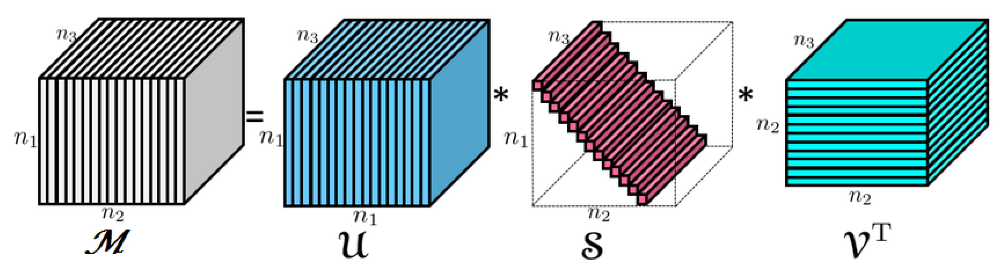
• the 3D tensors are considered as matrix of 1D vectors (tubes) and the approach uses a tensor product similar to the classical matrix product, after replacing multiplication of entries by, for example, convolution of the tubes,
• the SVD is fast to compute,
• a specific and natural nuclear norm can be easily defined.

Motivated by the 3D reconstruction problem, our goal in the present paper is to study the natural nuclear norm penalised estimator for tensor completion problem. Our approach extends the method proposed in [11] to the framework developed by [10]. The main contribution of the paper is

• to present the most natural definition of the nuclear norm in the framework of Reference [10],
• to compute the subdifferential of this nuclear norm,
• to present a precise mathematical study of the nuclear norm penalised least-squares reconstruction method,
• to illustrate the efficiency of the approach on the OCT reconstruction problem with real data.

1.2. Background on Tensor Completion

1.2.1. Matrix Completion

After the many successes of Compressed Sensing in inverse problems, Matrix and tensor completion problems have recently taken the stage and become the focus of an extensive research activity. Completion problems have applications in collaborative filtering [12], Machine Learning [13,14], sensor networks [15], subspace clustering [16], signal processing [8], and so forth. The problem is intractable if the matrix to recover does not have any particular structure. An important discovery in References [17,18] is that when the matrix to be recovered has a low rank, then it can be recovered based on a few observations only [18] and using nuclear norm penalised estimation is a reasonably easy problem to solve.

The use of the nuclear norm as a convex surrogate for the rank was first proposed in Reference [19] and further analysed in a series of breakthrough papers [3,11,17,20,21,22].

1.2.2. Tensor Completion

The matrix completion problem was recently generalised to the problem of tensor completion. A very nice overview of tensors and algorithms is given in Reference [23]. Tensors play a fundamental role in statistics [24] and more recently in Machine Learning [13]. It can be used for multidimensional time series [25], analysis of seismic data [6], Hidden Markov Models [13], Gaussian Mixture based clustering [26], Phylogenetics [27], and much more. Tensor completion is however a more difficult problem from many points of view. First, the rank is NP-hard to compute in full generality [5]. Second, many different Singular Value Decompositions are available. The Tucker decomposition [5] extends the useful sum of rank one decomposition to tensors but it is NP-hard to compute in general. An interesting algorithm was proposed in References [28,29]; see also the very interesting Reference [30]. Another SVD was proposed in Reference [31] with the main advantage that the generalized singular vectors form an orthogonal family. The usual diagonal matrix is replaced with a so called “core” tensor with nice orthogonality properties and very simple structure in the case of symmetric [32] or orthogonally decomposable tensors [33].

Another very interesting approach, called the t-SVD was proposed recently in [10] for 3D tensors with applications to face recognition [34] and image deblurring, computerized tomography [35] and data completion [36]. In the t-SVD framework, one dimension is assumed to be of a different nature from the others, such as, for example, time. In this setting, the decomposition resembles the SVD closely by using a diagonal tensor instead of a diagonal matrix as for the standard 2D SVD. The t-SVD was also proved to be amenable to online learning [37]. One other interesting advantage of the t-SVD is that the nuclear norm is well defined and its subdifferential is easy to compute.

The t-SVD proposed in Reference [10] is a very attractive representation of tensors in many settings such as image analysis, multivariate time series, and so forth. Obviously, it is not so attractive for the study of symmetric moment or cumulant tensors as studied in Reference [13], but for large image sequences and times series, this approach seems to be extremely relevant.

1.3. Sparsity

One of the main discoveries of the past decade is that sparsity may help in certain contexts where data are difficult or expensive to acquire [1]. When the object $A_0$ to recover is a vector, the fact that it may be sparse in a certain dictionary will dramatically improve recovery, as demonstrated by the recent breakthroughs in high dimensional statistics on the analysis of estimators obtained via convex optimization, such as the LASSO [38,39,40], the Adaptive LASSO [41] or the Elastic Net [42]. When $A_0$ is a matrix, the property of having a low rank may be crucial for the recovery as proved in References [11,43]. Extensions to the tensor case are studied in References [7,44,45]. Tensor completion using the t-SVD framework has been analyzed in Reference [36]. In particular, our results complement and improve on the results in Reference [36]. Reference [46] deserves special mention for using more advanced techniques based on real algebraic geometry and sums of squares decompositions.

The usual estimator in a sparse recovery problem is a nuclear norm penalized least squares such as the one studied here and defined by (27). Several other types of nuclear norms have been used for tensor estimation and completion. In particular, several nuclear norms can be naturally defined such as in for example, References [7,47,48]. It is interesting to notice that, sparsity promoting penalization of the least squares estimator crucially relies on the structure of the subdifferential of the norm involved. See for instance References [11,49] or Reference [50]. In Reference [7] a subset of the subdifferential is studied and then used in order to establish the efficiency of the penalized least squares approach. Another interesting approach is the one in [48] where an outer approximation of the subdifferential is given. In the matrix setting, the work in References [51,52] are famous for providing a neat characterization of the subdifferential of matrix norms or more generally functions of the matrix enjoying enough symmetries. In the 3D or higher dimensional setting, however, the case is much less understood. The relationship between the tensor norms and the norms of the flattening are intricate although some good bounds relating one to the other can be obtained, as, for example, in Reference [53].

The extension of previous results on low rank matrix reconstruction to the tensor setting is nontrivial but is shown to be relatively easy to obtain once the appropriate background is given. In particular, our theoretical analysis will generalise the analysis in Reference [11]. In order to do this, we provide a complete characterisation of the subdifferential of the nuclear norm. Our results will be illustrated by computational experiments for solving a problem in Optical Coherence Tomography (OCT).

1.4. Plan of the Paper

Section 2 presents the necessary mathematical background about tensors and sparse recovery. Section 3 introduces the measurement model and the present our nuclear-norm penalised estimator. In Section 4 we prove our main theoretical result. In Section 5, our approach is finally illustrated in the context of Optical Coherence Tomography, and some computational results based on real data are presented.

2. Background on Tensors, t-SVD

In this section, we present what is meant by the notion of tensor and the various generalisations of the common objects in linear algebra to the tensor setting. In particular, we will introduce the Singular Value Decomposition proposed in Reference [10] and some associated Schatten norms.

2.1. Basic Notations for Third-Order Tensor

In this section, we recall the framework introduced by Kilmer and Martin [9,10] for a very special class of tensors which is particularly adapted to our setting.

2.1.1. Slices and Transposition

For a third-order tensor A, its $\left(i,j,k\right)$th entry is denoted by A${}_{ijk}$.

Definition 1.

The kth-frontal slice of A is defined as

$$\begin{array}{cc}\hfill A^{\left(k\right)}& =A\left(:,:,k\right).\hfill \end{array}$$

The $jth$-transversal slice of A is defined as

$$\begin{array}{cc}\hfill {\overrightarrow{A}}^{\left(j\right)}& =A\left(:,j,:\right).\hfill \end{array}$$

A tubal scalar (t-scalar) is an element of ${\mathbb{R}}^{1\times 1\times n_3}$ and a tubal vector (t-vector) is an element of ${\mathbb{R}}^{n_1\times 1\times n_3}$.

Definition 2

(Tensor transpose). The conjugate transpose of a tensor $A\in {\mathbb{R}}^{n_1\times n_2\times n_3}$ tensor $A^t$ obtained by conjugate transposing each of the frontal slice and then reversing the order of transposed frontal slices starting from the slide number 2 to the slice number $n_3$ and then appending the conjugate transposed frontal slice $A^{{(1)}^{\top }}$.

Definition 3

(The “dot” product). The dot product $A·B$ between two tensors $A\in {\mathbb{R}}^{n_1\times n_2\times n_3}$ and $B\in {\mathbb{R}}^{n_2\times n_4\times n_3}$ is the tensor $C\in {\mathbb{R}}^{n_1\times n_4\times n_3}$ whose slice $C^{(n)}$ is the matrix product of the slice $A^{(n)}$ with the slice $B^{(n)}$:

$$\begin{array}{cc}\hfill C^{(k)}& :={(A·B)}^{(k)}:=A^{(k)}{B}^{(k)},k=1,\dots ,n_3.\hfill \end{array}$$

(1)

We will also need the canonical inner product.

Definition 4

(Inner product of tensors). If $\mathit{A}$ and $\mathit{B}$ are third-order tensors of same size $n_1\times n_2\times n_3$, then the inner product between A and B is defined as the following (notice the normalization constant of FFT),

$$\begin{array}{c}\hfill 〈A,B〉=\sum _{i=1}^{n_1}\sum _{j=1}^{n_2}\sum _{k=1}^{n_3}{A}_{ijk}{B}_{ijk}.\end{array}$$

(2)

2.1.2. Convolution and Fourier Transform

Definition 5

(t-product for circular convolution). The t-product $A\ast B$ of $A\in {\mathbb{R}}^{n_1\times n_2\times n_3}$ and $B\in {\mathbb{R}}^{n_2\times n_4\times n_3}$ is an $n_1\times n_4\times n_3$ tensor whose $\left(i,j\right)$-th tube is given by

$$\begin{array}{c}\hfill C\left(i,j,:\right)=\sum _{k=1}^{n_2}A\left(i,k,:\right)\ast B\left(k,j,:\right),\end{array}$$

(3)

where * denotes the circular convolution between two cubes of same size.

Definition 6

(Identity tensor). The identity tensor $J\in {\mathbb{R}}^{n_1\times n_1\times n_3}$ is defined to be a tensor whose first frontal slice $J^1$ is the $n_1\times n_1$ identity matrix and all other frontal slices $J^i,i=2,\dots ,n_3$ are zero.

Definition 7

(Orthogonal tensor). A tensor $Q\in {\mathbb{R}}^{n\times n\times n_3}$ is orthogonal if it satisfies

$$\begin{array}{c}\hfill Q^{\top }\ast Q=Q\ast Q^{\top }=J.\end{array}$$

(4)

$\widehat{A}$ is a tensor which is obtained by taking the Fast Fourier Transform (FFT) along the third dimension and we will use the following convention for Fast Transform along the 3rd dimension

$$\begin{array}{cc}\hfill \widehat{A}& =\mathrm{fft}\left(A,\left[\right],3\right).\hfill \end{array}$$

The one-dimensional FFT along the 3th-dimension is given

$$\begin{array}{c}\hfill \widehat{A}(j_1,j_2,k_3)=\sum _{j_3=1}^{n_3}A(j_1,j_2,j_3)exp(-2\frac{i\pi j_3{k}_3}{n_3}),\forall j_1,j_2,1⩽j_1⩽n_1,1⩽j_2⩽n_2.\end{array}$$

Naturally, one can compute A from $\widehat{A}$ via ifft$\left(\widehat{A},\left[\right],3\right)$ using the inverse FFT, and is defined:

$$\begin{array}{c}\hfill A(j_1,j_2,k_3)=\sum _{j_3=1}^{n_3}\widehat{A}(j_1,j_2,j_3)exp(2\frac{i\pi j_3{k}_3}{n_3}),\forall j_1,j_2,1⩽j_1⩽n_1,1⩽j_2⩽n_2.\end{array}$$

Definition 8

(Inverse of a tensor). The inverse of a tensor A$\in {\mathbb{R}}^{n\times n\times n_3}$ is written as $A^{-1}$ satisfying

$$\begin{array}{c}\hfill A^{-1}\ast A=A\ast A^{-1}=J.\end{array}$$

(5)

where J is the identity tensor of size $n\times n\times n_3$.

Remark 1.

It is proved in Reference [10] that for any tensor $A\in {\mathbb{R}}^{n_1\times n_2\times n_3}$ and $B\in {\mathbb{R}}^{n_2\times n_4\times n_3}$, we have

$$\begin{array}{c}\hfill A\ast B=C\iff \widehat{A}·\widehat{B}=\widehat{C}.\end{array}$$

2.2. The t-SVD

We finally arrive at the definition of the t-SVD.

Definition 9

(f-diagonal tensor). Tensor A is called f-diagonal if each frontal slice $A^{\left(i\right)}$ is a diagonal matrix.

Definition 10

(Tensor Singular Value Decomposition: t-SVD). For M $\in {\mathbb{R}}^{n_1\times n_2\times n_3}$, the t-SVD of M is given by

$$\begin{array}{c}\hfill M=U\ast S\ast V^{\top },\end{array}$$

(6)

where U and V are orthogonal tensor of size $n_1\times n_1\times n_3$ and $n_2\times n_2\times n_3$ respectively. S is a rectangular f-diagonal tensor or size $n_1\times n_2\times n_3$, and the entries in S are called the singular values of M. This SVD can be obtained using the Fourier transform as follows:

$$\begin{array}{cc}\hfill {\widehat{M}}^{(i)}& ={\widehat{U}}^{(i)}·{\widehat{S}}^{(i)}·{\left({\widehat{V}}^{(i)}\right)}^{\top }.\hfill \end{array}$$

(7)

This t-SVD is illustrated in Figure 1 below. Notice that the diagonal elements of S, i.e., $S(i,i,:)$ are tubal scalars as introduced in Definition 1. They will also be called tubal eigenvalues.

Definition 11.

The spectrum $\sigma (A)$ of the tensor A is the tubal vector given by

$$\begin{array}{cc}\hfill \sigma {(A)}_i& =S(i,i,:)\hfill \end{array}$$

(8)

for $i=1,\dots ,min\{n_1,n_2\}$.

2.3. Some Natural Tensor Norms

Using the previous definitions, it is easy to define some generalisations of the usual matrix norms.

Definition 12

(Tensor Frobenius norm). The induced Frobenius norm from the inner product defined above is given by,

$$\begin{array}{c}\hfill {\parallel A\parallel }_F={\langle A,A\rangle }^{1/2}=\frac{1}{\sqrt{n_3}}{\parallel \widehat{A}\parallel }_F=\sqrt{\sum _{i=1}^{n_1}\sum _{j=1}^{n_2}\sum _{k=1}^{n_3}\underset{ijk}{\overset{2}{A}}}.\end{array}$$

(9)

Definition 13

(Tensor spectral norm). The tensor spectral norm ${\parallel A\parallel }_{\infty }$ is defined as follows:

$$\begin{array}{c}\hfill {\parallel A\parallel }_{\infty }=\underset{i}{max}{\parallel \sigma {(A)}_i\parallel }_2\end{array}$$

(10)

where ${\parallel ·\parallel }_2$ is the $l_2$-norm.

Proposition 1.

Let M be $n_1\times n_2\times n_3$ tensor. Therefore

$$\begin{array}{c}\hfill {\parallel M\parallel }_{\infty }={\parallel \mathcal{F}(M)\parallel }_{\infty },\end{array}$$

where $\mathcal{F}$ corresponds to the Fast Fourier Transform.

Definition 14

(Tubal nuclear norm). The tensor nuclear norm of a tensor A denoted as ${\parallel A\parallel }_{⊛}$ is the sum of singular values of all the frontal slices of A. Moreover,

$$\begin{array}{cc}\hfill {\parallel A\parallel }_{⊛}& =\sum _{i=1}^{min\{n_1,n_2\}}\sqrt{\sum _{j=1}^{n_3}S{(i,i,j)}^2}\hfill \\ \hfill & =\sum _{i=1}^{min\{n_1,n_2\}}{\parallel \sigma {(A)}_i\parallel }_2.\hfill \end{array}$$

(11)

Note that by Parseval’s inequality

$$\begin{array}{cc}\hfill \sqrt{\sum _{j=1}^{n_3}S{(i,i,j)}^2}& =\frac{1}{\sqrt{n_3}}\sqrt{\sum _{j=1}^{n_3}\widehat{S}{(i,i,j)}^2}.\hfill \end{array}$$

(12)

Therefore, it is equivalent to define the tubal-nuclear norm via in the Fourier domain. Recall moreover that the $\widehat{S}(i,i,j)$ are all non-negative due to the fact that ${\widehat{U}}^{(k)}{\widehat{S}}^{(k)}{\widehat{V}}^{{(k)}^t}$ is the SVD of the $kth$ slice of A.

Proposition 2

(Trace duality property). Let A, B be $n_1\times n_2\times n_3$ tensor. Therefore

$$\begin{array}{c}\hfill \left|\langle A,B\rangle \right|⩽{\parallel A\parallel }_{⊛}{\parallel B\parallel }_{\infty }\end{array}$$

Proof. 

By Cauchy-Schwartz, we have

$$\begin{array}{ccc}\hfill |\langle A,B\rangle |& =\hfill & |\langle \mathcal{F}(A),\mathcal{F}(B)\rangle |\hfill \\ & =\hfill & |\langle \mathcal{F}(U)\mathcal{F}(S)\mathcal{F}(V^{\top }),\mathcal{F}(B)\rangle |\hfill \\ & =\hfill & \left|\sum _{i=1}^{n_3}\mathrm{tr}\left({\widehat{S}}^{(i)}{\widehat{V}}^{{(i)}^{\top }}\mathcal{F}{(B)}^{{(i)}^{\top }}{\widehat{U}}^{(i)}\right)\right|\hfill \\ & =\hfill & \left|\sum _{i=1}^{n_3}\sum _{j=1}^{min\{n_1,n_2\}}{\widehat{S}}_{jj}^{(i)}{\left({\widehat{V}}^{{(i)}^{\top }}\mathcal{F}{(B)}^{{(i)}^{\top }}{\widehat{U}}^{(i)}\right)}_{jj}\right|\hfill \\ & ⩽\hfill & \sum _{j=1}^{min\{n_1,n_2\}}{\left(\parallel {\widehat{S}}_{jj}{\parallel }_2\right)}^{1/2}{\left(\parallel {({\widehat{V}}^{\top }\mathcal{F}{(B)}^t\widehat{U})}_{jj}{\parallel }_2\right)}^{1/2}\hfill \\ & ⩽\hfill & \sum _{j=1}^{min\{n_1,n_2\}}{\left(\parallel {\widehat{S}}_{jj}{\parallel }_2\right)}^{1/2}{\left({\parallel \mathcal{F}(B)}_{jj}{\parallel }_2\right)}^{1/2},\hfill \end{array}$$

taking the maximum of ${\parallel \mathcal{F}(B)}_{jj}{\parallel }_2$ and the sum the slices of ${\left(\parallel {\widehat{S}}_{jj}{\parallel }_2\right)}^{1/2}$, and apply (12) and inverse of FFT, we obtain the result. □

Proposition 3.

Given tensor $A\in {\mathbb{R}}^{n_1\times n_2\times n_3}$. We have

$$\begin{array}{c}\hfill {\parallel A\parallel }_{⊛}⩽\sqrt{\mathrm{rank}(A)}{\parallel A\parallel }_F.\end{array}$$

Proof. 

Again by Cauchy-Schwartz, we have

$$\begin{array}{ccc}\hfill {\parallel A\parallel }_{⊛}& =\hfill & \sum _{j=1}^{min\{n_1,n_2\}}{\parallel S(j,j,:)\parallel }_2\hfill \\ & =\hfill & \sum _{j=1}^{\mathrm{rank}(\mathrm{A})}{\parallel S(j,j,:)\parallel }_2\hfill \\ & ⩽\hfill & \sqrt{\mathrm{rank}(A)}{\left(\sum _{j=1}^{min\{n_1,n_2\}}{\parallel S(j,j,;)\parallel }_2^2\right)}^{1/2}\hfill \\ & ⩽\hfill & \sqrt{\mathrm{rank}(A)}{\parallel A\parallel }_F.\hfill \end{array}$$

 □

Lemma 1.

We have

$$\begin{array}{c}\hfill \parallel P_{S_1^{\perp }}{\widehat{A}}^{\lambda }{P}_{S_2^{\perp }}{\parallel }_{⊛}=\underset{{\parallel W\parallel }_{\infty }⩽1}{max}\langle W,P_{S_1^{\perp }}{\widehat{A}}^{\lambda }{P}_{S_2^{\perp }}\rangle \end{array}$$

Proof. 

$$\begin{array}{ccc}\hfill \langle W,P_{S_1^{\perp }}{\widehat{A}}^{\lambda }{P}_{S_2^{\perp }}\rangle & =\hfill & \langle \mathcal{F}(W),\mathcal{F}(P_{S_1^{\perp }}{\widehat{A}}^{\lambda }{P}_{S_2^{\perp }})\rangle denoteB=\mathcal{F}(P_{S_1^{\perp }}{\widehat{A}}^{\lambda }{P}_{S_2^{\perp }})\mathrm{and}\mathrm{take}\mathrm{this}\mathrm{t}-\mathrm{svd}\hfill \\ & =\hfill & \sum _{i=1}^{n_3}\mathrm{tr}\left({\widehat{V}}^{{(i)}^{\top }}\mathcal{F}{(W)}^{{(i)}^{\top }}{\widehat{U}}^{(i)}{\widehat{S}}^{(i)}\right)\hfill \\ & =\hfill & \sum _{i=1}^{n_3}\sum _{j=1}^{min\{n_1,n_2\}}{\left({\widehat{V}}^{{(i)}^{\top }}\mathcal{F}{(W)}^{{(i)}^{\top }}{\widehat{U}}^{(i)}\right)}_{jj}{\widehat{S}}_{jj}^{(i)}\hfill \end{array}$$

If we take $\mathcal{F}(W)$ such as ${\left({\widehat{V}}^{\top }\mathcal{F}{(W)}^{\top }\widehat{U}\right)}_{jj}$ is colinear with ${\widehat{S}}_{jj}$, i.e, ∀, $j=1$, …, $min\{n_1,n_2\}$

$$\begin{array}{c}\hfill {\left({\widehat{V}}^{\top }\mathcal{F}{(W)}^{\top }\widehat{U}\right)}_{jj}={\alpha }_j{\widehat{S}}_{jj}\iff {\left(\widehat{V}{\widehat{S}}_W{\widehat{U}}^{\top }\right)}_{jj}={\alpha }_j{\widehat{S}}_{jj}\mathrm{with}{\alpha }_j⩽1.\end{array}$$

This means to solve the equation system to determine the ${\alpha }_j$. Thus,

$$\begin{array}{c}\hfill |{\alpha }_j\parallel {\widehat{S}}_{jj}{\parallel }_2|=1\Rightarrow |{\alpha }_j|=\frac{1}{\parallel {\widehat{S}}_{jj}{\parallel }_2}.\end{array}$$

With this result, the remaining of proof follows directly from the proof of Proposition 2. □

2.4. Rank, Range and Kernel

The rank, the range and the kernel are extremely important notions for matrices. They will play a role in our analysis of the penalised least squares tensor recovery procedure as well.

As noticed in Reference [10], a tubal scalar may have all its entrees different from zero but still be non-invertible. According to the definition, a tubal scalar $a\in {\mathbb{R}}^{1\times 1\times n_3}$ is invertible if there exists a tubal scalar b such that $a\ast b=b\ast a=e$. Equivalently, the Fourier transform $\widehat{a}$ of a has no coefficient equal to zero. We can define the tubal rank ${\rho }_i$ of $S_{i,i,:}$ as the number of non-zero components of $\widehat{S}(i,i,:)$. Then, the easiest way to define the rank of a tensor is by means of the notion of multirank as follows.

Definition 15.

The multirank of a tensor is the vector $({\rho }_1,\dots ,{\rho }_r)$ where r is the number of nonzero tubal vectors $S(i,i,:)$, $i=1,\dots ,min\{n_1,n_2\}$.

We now define the range of a tensor.

Definition 16.

Let j denote the number of invertible tubal eigenvalues and let k denote the number of nonzero noninvertible tubal eigenvalues. The range $\mathcal{R}(M)$ of a tensor $M\in {\mathbb{R}}^{n_1\times n_2\times n_3}$ is defined as

$$\begin{array}{cc}\hfill \mathcal{R}(M)& =\left\{{\overrightarrow{U}}^{(1)}\ast c_1+\cdots +{\overrightarrow{U}}^{(j+k)}\ast c_{j+k}\mid c_l\in \mathcal{R}ange(s_l\ast ·),l\in \{j+1,\cdots ,j+k\}\right\}.\hfill \end{array}$$

(13)

Definition 17.

Let j denote the number of invertible tubal eigenvalues. The kernel $\mathcal{K}(M)$ of a tensor $M\in {\mathbb{R}}^{n_1\times n_2\times n_3}$ is defined as

$$\begin{array}{cc}\hfill \mathcal{K}(M)& =\left\{{\overrightarrow{V}}^{(j+1)}\ast c_1+\cdots +{\overrightarrow{V}}^{(n_2)}\ast c_{n_2}\mid s_l\ast c_l=0,l\in \{j+1,\cdots ,j+n_2\}\right\}.\hfill \end{array}$$

(14)

3. Measurement Model and the Estimator

3.1. The Observation Model

In the model considered hereafter, the observed data are $Y_1$, …, $Y_n$ given by the following model

$$\begin{array}{c}\hfill Y_i=\langle X_i,A_0\rangle +{\xi }_i,i=1,\dots ,n,\end{array}$$

where the notation $\langle ·,·\rangle$ stands for the canonical scalar product of tensors. This can be seen as a tensor regression problem $X_i$, $i=1,\dots ,n$ are some tensors in ${\mathbb{R}}^{n_1\times n_2\times n_3}$ and ${\xi }_i$, $i=1,\dots ,n$ are some independent zero mean random variables. Assume that the frontal faces $X^{(i)}$ are i.i.d uniformly distributed on the set

$$\begin{array}{c}\hfill \mathcal{X}=\{e_j(n_1)e_k^{\top }(n_2),1⩽j⩽n_1,1⩽k⩽n_2\},\end{array}$$

(15)

where $e_k(n)$ are the canonical basis vectors in ${\mathbb{R}}^n$.

Our goal is to recover the tensor $A_0$ based on the data $Y_i$, $i=1,\dots ,n$ only for n as small as possible.

Definition 18.

For any tensors $A,B\in {\mathbb{R}}^{n_1\times n_2\times n_3}$, we define the scalar product

$$\begin{array}{cc}\hfill \langle A,B\rangle & =\sum _{i_1=1,\dots ,n_1}\sum _{i_2=1,\dots ,n_2}\sum _{i_3=1,\dots ,n_3}{A}_{i_1,i_2,i_3}{B}_{i_1,i_2,i_3},\hfill \end{array}$$

and the bilinear form

$$\begin{array}{c}\hfill {\langle A,B\rangle }_{L_2(\mathsf{\Pi })}=\frac{1}{n}\sum _{i=1}^n\mathbb{E}\left[\langle A,X_i\rangle \langle B,X_i\rangle \right]\end{array}$$

Here $\mathsf{\Pi }=\frac{1}{n}{\sum }_{i=1}^n{\mathsf{\Pi }}_i$, where ${\mathsf{\Pi }}_i$ denotes the distribution of $X_i$. The corresponding semi-norm ${\parallel A\parallel }_{L_2(\mathsf{\Pi })}^2$ is given by

$$\begin{array}{c}\hfill {\parallel A\parallel }_{L_2(\mathsf{\Pi })}^2=\frac{1}{n}\sum _{i=1}^n\mathbb{E}\left[{\langle A,X_i\rangle }^2\right]\end{array}$$

and will denote by M the tensor given by

$$\begin{array}{c}\hfill M=\frac{1}{n}\sum _{i=1}^n\left(Y_i{X}_i-\mathbb{E}\left[Y_i{X}_i\right]\right).\end{array}$$

3.2. The Estimator

The approach proposed in Reference [11] for low rank matrix estimation which will be extended to tensor estimation in the present paper consists in minimising

$$\begin{array}{cc}\hfill {\widehat{A}}_{\lambda }& \in {\mathrm{argmin}}_{A\in \mathbb{A}}{L}_n(A),\hfill \end{array}$$

(16)

where

$$\begin{array}{cc}\hfill L_n(A)& ={\parallel A\parallel }_{L_2(\mathsf{\Pi })}^2-〈\frac{2}{n}\sum _{i=1}^n{Y}_i{X}_i,A〉+\lambda {\parallel A\parallel }_{⊛},\hfill \end{array}$$

(17)

where ${\parallel ·\parallel }_{⊛}$ is a tubal tensor nuclear norm that we will introduce in Definition 14.

Recall that nuclear norm penalisation is widely used in sparse estimation when the matrix to be recovered is low rank [1]. Following the success of the application of sparsity to low rank matrix recovery, several extensions of the matrix nuclear norm were proposed in the literature [7,8,47], etc. Another type of nuclear norm was proposed in Reference [36] based on the tubal framework of Kilmer [10]. Our estimator is another nuclear norm penalisation based estimator. As it will be explained in Section 2 below, the nuclear norm used in the present paper has some advantages over other norms in the context of tubal low rank tensors and the resulting estimator is most relevant in many applications where we want to recover a tensor which is the sum of a small number of rank-one tensors.

4. Main Results

In this section, we provide our main results. First, in Section 4.2, we give a complete characterisation of the subdifferential of the nuclear norm (Definition 14). Then, we propose a statistical study of the nuclear-norm penalised estimator ${\widehat{A}}_{\lambda }$ in Section 4.3.

4.1. Preliminary Remarks

4.1.1. Orthogonal Invariance

It is easy to see that the t-nuclear norm is orthogonally invariant. Indeed, consider two orthogonal tensors $O_1\in {\mathbb{R}}^{n_1\times n_1\times n_3}$, $O_2\in {\mathbb{R}}^{n_2\times n_2\times n_3}$, $k=1,\dots ,n_3$. Since the product of two orthogonal tensors is itself orthogonal, we have

$$\begin{array}{cc}\hfill \sigma (A)& =\sigma (O_1\ast A\ast O_2^{\top }).\hfill \end{array}$$

(18)

4.1.2. Support of a Tensor

Given that the t-svd of a tensor is

$$\begin{array}{cc}\hfill A& =U\ast S\ast V^{\top }\hfill \end{array}$$

(19)

$$\begin{array}{cc}\hfill & =\sum _{k=1}^{min\{n_1,n_2\}}{\overrightarrow{U}}^{(k)}\ast {\overrightarrow{s}}_{kk}\ast {\overrightarrow{V}}^{{(k)}^{\top }},\hfill \end{array}$$

(20)

with $({\overrightarrow{U}}^{(1)},\dots ,{\overrightarrow{U}}^{(min\{n_1,n_2\})})$ is a family of orthonormal matrix in ${\mathbb{R}}^{n_1\times n_1}$, and $({\overrightarrow{V}}^{(1)},\dots ,{\overrightarrow{V}}^{(min\{n_1,n_2\})})$ a family of orthonormal matrix in ${\mathbb{R}}^{n_2\times n_2}$ and ${\overrightarrow{s}}_{kk}=S(k,k,:)$ are the spectrum of A.

The support of A is the couple of linear vector spaces $(S_1,S_2)$ of tubal tensors, where

• $S_1$ is the linear span of $({\overrightarrow{U}}^{(1)},\dots ,{\overrightarrow{U}}^{(min\{n_1,n_2\})})$ and
• $S_2$ is the linear span of $({\overrightarrow{V}}^{(1)},\dots ,{\overrightarrow{V}}^{(min\{n_1,n_2\})})$.

We also let $S_j^{\perp },j=1,2$ to be the orthogonal complements of $S_j$ and by $P_{S_j},j=1,2$, the projector on linear vector subspace S of tubal tensors.

4.2. The Subdifferential of the t-nuclear Norm

Our first result is a characterisation of the subdifferential of ${\parallel ·\parallel }_{⊛}$. Recall first the particular case of the matrix nuclear norm ${\parallel ·\parallel }_{\ast }$. By Corollary 2.5 in [52], we have

$$\begin{array}{c}\hfill {\partial \parallel ·\parallel }_{\ast }=\{U{V}^t+W|\parallel W\parallel ⩽1,U^{t}W=0,VW=0\}.\end{array}$$

This result is established in [52] using the Von-Neumann inequality and in particular the equality case of this inequality.

4.2.1. Von-Neumann’s Inequality for Tubal Tensors

Theorem 1.

Let A, B be $n_1\times n_2\times n_3$ tensor. Therefore

$$\begin{array}{c}\hfill \langle A,B\rangle ⩽\langle S^A,S^B\rangle \end{array}$$

(21)

where $S^A$ is a rectangular f-diagonal tensor, contains all the singular values of A.

Equality holds in (21) if and only if A, B have the same singular tensors.

Proof. 

Let $\mathcal{F}$ denote the Fast Fourier Transform. We have

$$\begin{array}{ccc}\hfill \langle A,B\rangle & =\hfill & \langle \mathcal{F}\left(A\right),\mathcal{F}\left(B\right)\rangle \hfill \\ & =\hfill & 〈\mathcal{F}\left(U^A\ast S^A\ast \left(V^{A^{\top }}\right)\right),\mathcal{F}\left(U^B\ast S^B\ast \left(V^{B^{\top }}\right)\right)〉\hfill \\ & =\hfill & 〈\mathcal{F}\left(U^A\right)·\mathcal{F}\left(S^A\right)·F\left(V^{A^{\top }}\right),\mathcal{F}\left(U^B\right)·\mathcal{F}\left(S^B\right)·\mathcal{F}\left(V^{B^{\top }}\right)〉\hfill \\ & =\hfill & \sum _{k=1}^{n_3}\langle \mathcal{F}{\left(U^A\right)}^{\left(k\right)}·\mathcal{F}{\left(S^A\right)}^{\left(k\right)}·{\left(\mathcal{F}\left(V^{A^{\top }}\right)\right)}^{\left(k\right)},\hfill \\ & & \mathcal{F}{\left(U^B\right)}^{\left(k\right)}·\mathcal{F}{\left(S^B\right)}^{\left(k\right)}·{\left(\mathcal{F}\left(V^{B^{\top }}\right)\right)}^{\left(k\right)}\rangle .\hfill \end{array}$$

Thus, using the Von Neumann inequality for matrices, we get

$$\begin{array}{cc}⩽& \sum _{k=1}^{n_3}\langle \mathcal{F}{\left(S^A\right)}^{\left(k\right)},\mathcal{F}{\left(S^B\right)}^{\left(k\right)}\rangle \hfill \\ ⩽& \langle \mathcal{F}\left(S^A\right),\mathcal{F}\left(S^B\right)\rangle \hfill \\ =& \langle S^A,S^B\rangle ,\hfill \end{array}$$

where the last equality stems from the isometry property of Fast Fourier Transform. □

Notice that the Von-Neumann inequality was extended in [54] to general tensors and exploited in [55] for the computation of the subdifferential of some tensor norms. In comparison, the case of the t-nuclear norm only need an appropriate use of the matrix Von Neumann inequality.

4.2.2. Lewis’s Characterization of the Subdifferential

Theorem 2.

Let $f:{\mathbb{R}}^{min\{n_1,n_2\}}\mapsto \mathbb{R}$ be a function convex, so:

$$\begin{array}{c}\hfill {\left(f\circ \sigma \right)}^{\ast }=f^{\ast }\circ \sigma .\end{array}$$

The proof is exactly the same as in [52], Theorem 2.4.

Theorem 3.

Let us suppose that the function $f:{\mathbb{R}}^{min\{n_1,n_2\}}⟶\mathbb{R}$ is convex. Then, the tensor

$$\begin{array}{c}\hfill Y\in \partial \left(f\circ \sigma \right)\left(X\right)\mathit{if}\mathit{and}\mathit{only}\mathit{if}\sigma \left(Y\right)\in \partial f\left(\sigma \left(X\right)\right).\end{array}$$

(22)

The proof is the same as in [52], Corollary 2.5 where the matrix Von Neumann inequality (and more precisely, the exact characterization of the equality case) is replaced with Von Neumann inequality for tubal tensors given by Theorem 4.1.

Theorem 4.

Let r denote the number of ${\overrightarrow{S}}_X^{(k)}$ which are non-zero. The subdifferential of the t-nuclear norm is given by

$$\begin{array}{cc}\hfill {\partial \parallel X\parallel }_{⊛}& =\{U\ast D(\overrightarrow{\mu })\ast V^t+W|{\overrightarrow{\mu }}_k={\overrightarrow{S}}_X^{(k)}/{\parallel {\overrightarrow{S}}_X^{(k)}\parallel }_2,k=1,\dots ,r,\hfill \\ \hfill & \parallel {\overrightarrow{\mu }}_k{\parallel }_2=1,r<k⩽min\{n_1,n_2\}\}.\hfill \end{array}$$

(23)

Proof. 

We only need to rewrite (22) using the well-known formula for the subdifferential of the Euclidean norm. We provide the details for the sake of completeness.

Let ${\overrightarrow{S}}_X$ be a t-vector in ${\mathbb{R}}^{n_1\times 1\times n_3}$.

$$\begin{array}{ccc}\hfill \partial f(\sigma (X))& =\hfill & \partial \left(\sum _{k=1}^{min\{n_1,n_2\}}{\parallel {\overrightarrow{S}}_X^{(k)}\parallel }_2\right)\hfill \\ & =\hfill & \partial \parallel {\overrightarrow{S}}_X^{(1)}{\parallel }_2\times \dots \times {\parallel {\overrightarrow{S}}_X^{(min\{n_1,n_2\})}\parallel }_2\hfill \end{array}$$

(24)

where in second equality we use the result of [56], Chapter 16,l Section 1, Proposition 16.8.

As is well known, the subgradient of the $l_2$-norm is

$${\partial \parallel w\parallel }_2=\left\{\begin{array}{ccc}\left\{\frac{w}{{\parallel w\parallel }_2}\right\}& if& w\ne 0\\ \{z,\parallel z{\parallel }_2⩽1\}& if& w=0\end{array}\right.$$

and plugg this formula into (24). Therefore

$$\begin{array}{ccc}\hfill \partial (f\circ \sigma )(X)& =\{U\ast D(\overrightarrow{\mu })\ast V^{\top }|\overrightarrow{\mu }\in \partial f(\sigma (X)),U\in {\mathbb{R}}^{n_1\times n_1\times n_3},V\in {\mathbb{R}}^{n_2\times n_2\times n_3},\hfill & \hfill X=U\ast S\ast V^{\top }\}.\end{array}$$

(25)

Let T be the set of indices j which tubal scalar $\sigma {(X)}_j\ne 0$. Thus,

$$\begin{array}{c}\hfill U\ast D(\overrightarrow{\mu })\ast V^{\top }=U_T\ast D({\overrightarrow{\mu }}_T)\ast V_T^{\top }+U_{T^c}\ast D({\overrightarrow{\mu }}_{T^c})\ast V_{T^c}^{\top }\end{array}$$

Moreover,

$$\begin{array}{c}\hfill {\overrightarrow{\mu }}_T=\left[\begin{array}{c}\frac{{\overrightarrow{S}}_X^{(1)}}{\parallel {\overrightarrow{S}}_X^{(1)}{\parallel }_2}\\ ⋮\\ \frac{{\overrightarrow{S}}_X^{(min\{n_1,n_2\})}}{\parallel {\overrightarrow{S}}_X^{(min\{n_1,n_2\})}{\parallel }_2}\end{array}\right].\end{array}$$

(26)

Therefore, $U\ast D(\overrightarrow{\mu })\ast V^{\top }$ is of the form

$$\begin{array}{c}\hfill U_T\ast D({\overrightarrow{\mu }}_T)\ast V_T^{\top }+W\end{array}$$

with $W=U_{T^c}\ast D({\overrightarrow{\mu }}_{T^c})\ast V_{T^c}^{\top }$ and

$$\begin{array}{c}\hfill {\overrightarrow{\mu }}_{T^c}\in {\{z,\parallel z\parallel }_2{⩽1\}}^{\times |T^c|}.\end{array}$$

So we have,

$$\begin{array}{cc}\hfill {\parallel W\parallel }_{\infty }⩽1,U_T^{\top }\ast W& =0\mathrm{and}W\ast V_T=0.\hfill \end{array}$$

 □

4.3. Error Bound

Our error bound on tubal-tensor recovery using the approach of Koltchinskii, Lounici and Tsybakov [11] is given in the following theorem.

Theorem 5.

Let $\mathbb{A}\subseteq {\mathbb{R}}^{n_1\times n_2\times n_3}$ be a convex set of tensors. Let ${\widehat{A}}^{\lambda }$ be defined by

$$\begin{array}{cc}\hfill {\widehat{A}}^{\lambda }& =\underset{A\in \mathbb{A}}{arg\; min}{\parallel A\parallel }_{L_2(\mathsf{\Pi })}^2-2〈\frac{1}{n}\sum _{i=1}^n{Y}_i{X}_i,A〉+\lambda {\parallel A\parallel }_{⊛},\hfill \end{array}$$

(27)

where we recall that ${\parallel ·\parallel }_{⊛}$ denotes the tensor nuclear norm (see Definition 14). Assume that there exists a constant $\rho >0$ such that, for all tensor $A\in \mathbb{A}-\mathbb{A}:=\{A_1-A_2:A_1,A_2\in \mathbb{A}\}$,

$$\begin{array}{c}\hfill {\parallel A\parallel }_{L_2(\mathsf{\Pi })}^2\ge {\rho }^{-2}{\parallel A\parallel }_F^2.\end{array}$$

(28)

Let $\lambda \ge {2\parallel M\parallel }_{\infty }$, then

$$\begin{array}{c}\hfill \parallel {\widehat{A}}^{\lambda }-A_0{\parallel }_{L_2(\mathsf{\Pi })}^2⩽\underset{A\in \mathbb{A}}{inf}\left[\parallel A-A_0{\parallel }_{L_2(\mathsf{\Pi })}^2+{\left(\frac{1+\sqrt{2}}{2}\right)}^2{\rho }^2{\lambda }^2\mathrm{rank}(A)\right].\end{array}$$

Proof. 

We follow the proof of Reference [11]. We provide all the details for the sake of the completeness.

$$\begin{array}{c}\hfill {\widehat{A}}^{\lambda }\in \underset{A\in \mathbb{A}}{arg\; min}{L}_n({\widehat{A}}^{\lambda })={\parallel A\parallel }_{L_2(\mathsf{\Pi })}^2-2〈\frac{1}{n}\sum _{i=1}^n{Y}_i{X}_i,A〉+\lambda {\parallel A\parallel }_{⊛}.\end{array}$$

(29)

Let us compute the directional derivative of $L_n$ at ${\widehat{A}}^{\lambda }$.

$$\begin{array}{c}\hfill D{L}_n({\widehat{A}}^{\lambda };h)=\underset{t\to 0}{lim}\frac{L_n({\widehat{A}}^{\lambda }+th)-L_n({\widehat{A}}^{\lambda })}{t}.\end{array}$$

The optimality condition of ${\widehat{A}}^{\lambda }$ implies $D{L}_n({\widehat{A}}^{\lambda };A-{\widehat{A}}^{\lambda })\ge 0,\forall A\in \mathbb{A}$. Thus

$$\begin{array}{ccc}\hfill L_n({\widehat{A}}^{\lambda }+th)& =\hfill & \parallel {\widehat{A}}^{\lambda }{+th\parallel }_{L_2(\mathsf{\Pi })}^2-2〈\frac{1}{n}\sum _{i=1}^n{Y}_i{X}_i,{\widehat{A}}^{\lambda }+th〉+\lambda {\parallel {\widehat{A}}^{\lambda }+th\parallel }_{⊛}\hfill \\ & =\hfill & {\parallel A\parallel }_{L_2(\mathsf{\Pi })}^2+2t{\langle {\widehat{A}}^{\lambda },h\rangle }_{L_2(\mathsf{\Pi })}+t^2{\parallel h\parallel }_{L_2(\mathsf{\Pi })}^2-2〈\frac{1}{n}\sum _{i=1}^n{Y}_i{X}_i,{\widehat{A}}^{\lambda }〉\hfill \\ & & -2t〈\frac{1}{n}\sum _{i=1}^n{Y}_i{X}_i,h〉+\lambda {\parallel {\widehat{A}}^{\lambda }+th\parallel }_{⊛}\hfill \end{array}$$

$$\begin{array}{cc}\hfill \underset{t\to 0}{lim}\frac{L_n(A+th)-L_n(A)}{t}& =2{\langle {\widehat{A}}^{\lambda },h\rangle }_{L_2(\mathsf{\Pi })}-2〈\frac{1}{n}\sum _{i=1}^n{Y}_i{X}_i,h〉\hfill \\ \hfill & +\lambda \left(\parallel {\widehat{A}}^{\lambda }{+th\parallel }_{⊛}-{\parallel {\widehat{A}}^{\lambda }\parallel }_{⊛}\right)\ge 0\hfill \end{array}$$

for all $h\in T_{\mathbb{A}}({\widehat{A}}^{\lambda })$ (the tangent cone to $\mathbb{A}$ at ${\widehat{A}}^{\lambda }$). Taking $h=A-{\widehat{A}}^{\lambda }$, we have,

$$\begin{array}{c}\hfill 2{\langle {\widehat{A}}^{\lambda },A-{\widehat{A}}^{\lambda }\rangle }_{L_2(\mathsf{\Pi })}-2〈\frac{1}{n}\sum _{i=1}^n{Y}_i{X}_i,A-{\widehat{A}}^{\lambda }〉+\lambda \underset{t\to 0}{lim}\left(\frac{\parallel {\widehat{A}}^{\lambda }{+th\parallel }_{⊛}-{\parallel {\widehat{A}}^{\lambda }\parallel }_{⊛}}{t}\right)\ge 0.\end{array}$$

(30)

On the other hand,

$$\begin{array}{ccc}\hfill \underset{t\to 0}{lim}\left(\frac{\parallel {\widehat{A}}^{\lambda }{+th\parallel }_{⊛}-{\parallel {\widehat{A}}^{\lambda }\parallel }_{⊛}}{t}\right)& =\hfill & \underset{G\in \partial \parallel ·\parallel ({\widehat{A}}^{\lambda })}{max}\langle G,A-{\widehat{A}}^{\lambda }\rangle \hfill \\ & =\hfill & \langle {\widehat{G}}^{\lambda },A-{\widehat{A}}^{\lambda }\rangle \hfill \end{array}$$

(31)

by compacity of $G\in {\partial \parallel ·\parallel }_{⊛}({\widehat{A}}^{\lambda })$; see [57]. Combining (31) with (26), we obtain

$$\begin{array}{cc}\hfill 2{\langle {\widehat{A}}^{\lambda },{\widehat{A}}^{\lambda }-A\rangle }_{L_2(\mathsf{\Pi })}-2〈\frac{1}{n}\sum _{i=1}^n{Y}_i{X}_i,{\widehat{A}}^{\lambda }-A〉+\lambda \langle \widehat{G},{\widehat{A}}^{\lambda }-A\rangle & \le 0.\hfill \end{array}$$

(32)

Consider an arbitrary tensor $A\in \mathbb{A}$ of tubal rank r with spectral representation

$$\begin{array}{cc}\hfill A& =U\ast S\ast V^t=\sum _{j=1}^r{\overrightarrow{U}}^{(j)}\ast {\overrightarrow{s}}_{jj}\ast {\overrightarrow{V}}^{{(j)}^t}\hfill \end{array}$$

(33)

where ${\overrightarrow{s}}_{jj}=S\left(j,j,:\right)$, and with support $\left(S_1,S_2\right)$. Using that

$$\begin{array}{cc}\hfill 〈\frac{1}{n}\sum _{i=1}^n\mathbb{E}\left[Y_i{X}_i\right],{\widehat{A}}^{\lambda }-A〉& ={\langle A_0,{\widehat{A}}^{\lambda }-A\rangle }_{L_2(\mathsf{\Pi })}\hfill \end{array}$$

(34)

it thus follows from (32) that

$$\begin{array}{c}\hfill 2{\langle {\widehat{A}}^{\lambda }-A_0,{\widehat{A}}^{\lambda }-A\rangle }_{L_2(\mathsf{\Pi })}+\lambda \langle {\widehat{G}}^{\lambda }-G,{\widehat{A}}^{\lambda }-A\rangle ⩽-\lambda \langle G,{\widehat{A}}^{\lambda }-A\rangle +2\langle M,{\widehat{A}}^{\lambda }-A\rangle \end{array}$$

(35)

with

$$\begin{array}{c}\hfill M=\frac{1}{n}\sum _{i=1}^n\left(Y_i{X}_i-\mathbb{E}\left[Y_i{X}_i\right]\right).\end{array}$$

By the monotonicity of subdifferentials of convex functions, we have $\langle \widehat{G}-G,{\widehat{A}}^{\lambda }-A\rangle \ge 0$ (cf. [58], Chapter 4, Section 3, Proposition 9). Therefore

$$\begin{array}{c}\hfill 2{\langle {\widehat{A}}^{\lambda }-A_0,{\widehat{A}}^{\lambda }-A\rangle }_{L_2(\mathsf{\Pi })}⩽-\lambda \langle G,{\widehat{A}}^{\lambda }-A\rangle +2\langle M,{\widehat{A}}^{\lambda }-A\rangle .\end{array}$$

(36)

Furthermore, by (23), the following representations holds

$$\begin{array}{c}\hfill G=\sum _{j=1}^r{\overrightarrow{U}}^{(j)}\ast {\overrightarrow{\mu }}_j\ast {\overrightarrow{V}}^{{(j)}^{\top }}+P_{S_1^{\perp }}W{P}_{S_2^{\perp }}\end{array}$$

where W is an arbitrary tensor with ${\parallel W\parallel }_{\infty }⩽1$ and

$$\begin{array}{ccc}\hfill \langle P_{S_1^{\perp }}W{P}_{S_2^{\perp }},{\widehat{A}}^{\lambda }-A\rangle & =\hfill & \langle P_{S_1^{\perp }}W{P}_{S_2^{\perp }},{\widehat{A}}^{\lambda }\rangle \hfill \\ & =\hfill & \langle W,P_{S_1^{\perp }}{\widehat{A}}^{\lambda }{P}_{S_2^{\perp }}\rangle \hfill \end{array}$$

and using Lemma 3, we can choose W such that

$$\begin{array}{c}\hfill \langle P_{S_1^{\perp }}W{P}_{S_2^{\perp }},{\widehat{A}}^{\lambda }-A\rangle ={\parallel P_{S_1^{\perp }}{\widehat{A}}^{\lambda }{P}_{S_2^{\perp }}\parallel }_{⊛},\end{array}$$

where in the first equality we used that A has support $\left(S_1,S_2\right).$ For this particular choice of W, (36) implies that

$$\begin{array}{cc}\hfill 2{\langle {\widehat{A}}^{\lambda }-A_0,{\widehat{A}}^{\lambda }-A\rangle }_{L_2(\mathsf{\Pi })}+\lambda {\parallel P_{S_1^{\perp }}{\widehat{A}}^{\lambda }{P}_{S_2^{\perp }}\parallel }_{⊛}& ⩽-\lambda 〈\sum _{j=1}^r{\overrightarrow{U}}^{(j)}\ast {\overrightarrow{\mu }}_j\ast {\overrightarrow{V}}^{{(j)}^{\top }},{\widehat{A}}^{\lambda }-A〉\hfill \\ \hfill & +2\langle M,{\widehat{A}}^{\lambda }-A\rangle \hfill \end{array}$$

(37)

Using the identity

$$\begin{array}{c}\hfill 2{\langle {\widehat{A}}^{\lambda }-A_0,{\widehat{A}}^{\lambda }-A\rangle }_{L_2(\mathsf{\Pi })}=\parallel {\widehat{A}}^{\lambda }-A_0{\parallel }_{L_2(\mathsf{\Pi })}^2+\parallel {\widehat{A}}^{\lambda }{-A\parallel }_{L_2(\mathsf{\Pi })}^2-{\parallel A-A_0\parallel }_{L_2(\mathsf{\Pi })}^2\end{array}$$

and the fact that

$$\begin{array}{c}\hfill \parallel \sum _{j=1}^r{\overrightarrow{U}}^{(j)}\ast {\overrightarrow{\mu }}_j\ast {\overrightarrow{V}}^{{(j)}^{\top }}{\parallel }_{\infty }={\parallel D(\overrightarrow{\mu })\parallel }_{\infty }\end{array}$$

$$\begin{array}{c}\hfill 〈\sum _{j=1}^r{\overrightarrow{U}}^{(j)}\ast {\overrightarrow{\mu }}_j\ast {\overrightarrow{V}}^{{(j)}^{\top }},{\widehat{A}}^{\lambda }-A〉=〈\sum _{j=1}^r{\overrightarrow{U}}^{(j)}\ast {\overrightarrow{\mu }}_j\ast {\overrightarrow{V}}^{{(j)}^{\top }},P_{S_1}\left({\widehat{A}}^{\lambda }-A\right)P_{S_2}〉\end{array}$$

we deduce from (37) that

$$\begin{array}{c}\hfill \parallel {\widehat{A}}^{\lambda }-A_0{\parallel }_{L_2(\mathsf{\Pi })}^2+\parallel {\widehat{A}}^{\lambda }{-A\parallel }_{L_2(\mathsf{\Pi })}^2+\lambda {\parallel P_{S_1^{\perp }}{\widehat{A}}^{\lambda }{P}_{S_2^{\perp }}\parallel }_{⊛}⩽\parallel A-A_0{\parallel }_{L_2(\mathsf{\Pi })}^2\\ \hfill \\ \hfill +\lambda \parallel D(\overrightarrow{\mu }){\parallel }_{\infty }{\parallel P_{S_1}({\widehat{A}}^{\lambda }-A)P_{S_2}\parallel }_{⊛}+2\langle M,{\widehat{A}}^{\lambda }-A\rangle .\end{array}$$

(38)

Now, to find an upper bound on $2\langle M,{\widehat{A}}^{\lambda }-A\rangle$, we use the following decomposition:

$$\begin{array}{ccc}\hfill \langle \mathrm{M},{\widehat{A}}^{\lambda }-A\rangle & =\hfill & \langle {\mathcal{P}}_A(\mathrm{M}),{\widehat{A}}^{\lambda }-A\rangle +\langle P_{S_1^{\perp }}\mathrm{M}{P}_{S_2^{\perp }},{\widehat{A}}^{\lambda }-A\rangle \hfill \\ & =\hfill & \langle {\mathcal{P}}_A(\mathrm{M}),{\mathcal{P}}_A({\widehat{A}}^{\lambda }-A)\rangle +\langle P_{S_1^{\perp }}\mathrm{M}{P}_{S_2^{\perp }},{\widehat{A}}^{\lambda }\rangle \hfill \end{array}$$

where ${\mathcal{P}}_A(M)=M-P_{S_1^{\perp }}M{P}_{S_2^{\perp }}$. This implies, due to the trace duality,

$$\begin{array}{ccc}\hfill 2|\langle \mathrm{M},{\widehat{A}}^{\lambda }-A\rangle |& =\hfill & 2|\langle {\mathcal{P}}_A(M),{\mathcal{P}}_A({\widehat{A}}^{\lambda }-A)\rangle +\langle P_{S_1^{\perp }}\mathrm{M}{P}_{S_2^{\perp }},{\widehat{A}}^{\lambda }\rangle |\hfill \\ \hfill & ⩽\hfill & 2|\langle {\mathcal{P}}_A(M),{\mathcal{P}}_A({\widehat{A}}^{\lambda }-A)\rangle |+2|\langle P_{S_1^{\perp }}\mathrm{M}{P}_{S_2^{\perp }},{\widehat{A}}^{\lambda }\rangle |\hfill \\ \hfill & ⩽\hfill & 2\parallel {\mathcal{P}}_A{(M)\parallel }_F\parallel {\mathcal{P}}_A({\widehat{A}}^{\lambda }-A){\parallel }_F+2\parallel P_{S_1^{\perp }}\mathrm{M}{P}_{S_2^{\perp }}{\parallel }_{\infty }{\parallel P_{S_1^{\perp }}{\widehat{A}}^{\lambda }{P}_{S_2^{\perp }}\parallel }_{⊛}\hfill \\ & ⩽\hfill & \mathsf{\Lambda }\parallel {\widehat{A}}^{\lambda }{-A\parallel }_F+\mathsf{\Gamma }{\parallel P_{S_1^{\perp }}{\widehat{A}}^{\lambda }{P}_{S_2^{\perp }}\parallel }_{⊛}\hfill \end{array}$$

(39)

where

$$\begin{array}{c}\hfill \mathsf{\Lambda }=2\parallel {\mathcal{P}}_A{(M)\parallel }_F,\mathrm{and}\mathsf{\Gamma }=2{\parallel P_{S_1^{\perp }}\mathrm{M}{P}_{S_2^{\perp }}\parallel }_{\infty }\end{array}$$

Using that

$$\begin{array}{c}\hfill {\mathcal{P}}_A(\mathrm{M})=P_{S_1^{\perp }}\mathrm{M}{P}_{S_2}+P_{S_1}\mathrm{M}\mathrm{and}\mathrm{rank}(P_{S_j})⩽\mathrm{rank}(A),j=1,2\end{array}$$

we have with $\mathsf{\Delta }={\parallel M\parallel }_{\infty }$

$$\begin{array}{c}\hfill \mathsf{\Lambda }⩽2\sqrt{\mathrm{rank}({\mathcal{P}}_A)(\mathrm{M})}{\parallel \mathrm{M}\parallel }_{\infty }⩽2\sqrt{2\mathrm{rank}(A)}\mathsf{\Delta }⩽\sqrt{2\mathrm{rank}(A)}\lambda \end{array}$$

Thus,

$$\begin{array}{cc}\hfill 2|\langle \mathrm{M},{\widehat{A}}^{\lambda }-A\rangle |& ⩽\sqrt{2\mathrm{rank}(A)}\lambda \parallel {\widehat{A}}^{\lambda }{-A\parallel }_F+2\mathsf{\Delta }{\parallel P_{S_1^{\perp }}{\widehat{A}}^{\lambda }{P}_{S_2^{\perp }}\parallel }_{⊛}\hfill \end{array}$$

(40)

Due to Proposition 3, we have

$$\begin{array}{ccc}\hfill \parallel P_{S_1}({\widehat{A}}^{\lambda }-A)P_{S_2}{\parallel }_{⊛}& ⩽\sqrt{\mathrm{rank}({\widehat{A}}^{\lambda }-A)}{\parallel P_{S_1}({\widehat{A}}^{\lambda }-A)P_{S_2}\parallel }_F\hfill & \hfill ⩽\sqrt{\mathrm{rank}({\widehat{A}}^{\lambda }-A)}{\parallel {\widehat{A}}^{\lambda }-A\parallel }_F\end{array}$$

(41)

and using the assumption (28), it follows from (38) and (40) that

$$\begin{array}{c}\hfill \parallel {\widehat{A}}^{\lambda }-A_0{\parallel }_{L_2(\mathsf{\Pi })}^2+\parallel {\widehat{A}}^{\lambda }{-A\parallel }_{L_2(\mathsf{\Pi })}^2+(\lambda -2\mathsf{\Delta })\parallel P_{S_1^{\perp }}{\widehat{A}}^{\lambda }{P}_{S_2^{\perp }}{\parallel }_{⊛}⩽{\parallel A-A_0\parallel }_{L_2(\mathsf{\Pi })}^2+\\ \hfill +\left(\parallel D(\overrightarrow{\mu }){\parallel }_{\infty }+\sqrt{2}\right)\rho \lambda \sqrt{\mathrm{rank}(A)}{\parallel {\widehat{A}}^{\lambda }-A\parallel }_{L_2(\mathsf{\Pi })}\end{array}$$

(42)

Using

$$\begin{array}{cc}\hfill & \left(\parallel D(\overrightarrow{\mu }){\parallel }_{\infty }+\sqrt{2}\right)\rho \lambda \sqrt{\mathrm{rank}(A)}\parallel {\widehat{A}}^{\lambda }{-A\parallel }_{L_2(\mathsf{\Pi })}-{\parallel {\widehat{A}}^{\lambda }-A\parallel }_{L_2(\mathsf{\Pi })}^2\hfill \\ \hfill & ⩽\frac{1}{4}{\left(\parallel D(\overrightarrow{\mu }){\parallel }_{\infty }+\sqrt{2}\right)}^2{\rho }^2{\lambda }^2\mathrm{rank}(A),\hfill \end{array}$$

we deduce from (42) that

$$\begin{array}{cc}\hfill \parallel {\widehat{A}}^{\lambda }-A_0{\parallel }_{L_2(\mathsf{\Pi })}^2+(\lambda -2\mathsf{\Delta }){\parallel P_{S_1^{\perp }}{\widehat{A}}^{\lambda }{P}_{S_2^{\perp }}\parallel }_{⊛}& ⩽\parallel A-A_0{\parallel }_{L_2(\mathsf{\Pi })}^2\hfill \\ & \hfill \\ \hfill & +\frac{1}{4}{\left(\parallel D(\overrightarrow{\mu }){\parallel }_{\infty }+\sqrt{2}\right)}^2{\rho }^2{\lambda }^2\mathrm{rank}(A)\hfill \end{array}$$

 □

In Appendix A, it is proved that we can set

$$\begin{array}{cc}\hfill \rho & =\sqrt{m{n}_1{n}_2{n}_3^{3/2}}\hfill \end{array}$$

(43)

and

$$\begin{array}{cc}\hfill \lambda & =2n_3{\parallel \mathcal{F}(A_0)\parallel }_{S_{\infty }}max\left\{\sqrt{\frac{t+log(m)}{n{n}_1{n}_2}};\left(1+\frac{1}{\sqrt{n_1{n}_2}}\right)\frac{t+log(m)}{n}\right\}.\hfill \end{array}$$

(44)

5. Numerical Experiments

The proposed methods were numerically validated using 3D OCT images. OCT is widely studied as a medical imaging system in many clinical applications and fundamental research. In numerous clinical purposes, OCT is considered as a very interesting technique for in situ tissue characterization known as “optical biopsy” (in opposition to the conventional physical biopsy). OCT is operating under the principle of low coherence interferometry providing micro-meter spatial resolution at several MHz A-scan (1D optical core in z direction) acquisition rate. In these experiments, we found that depth was a different coordinate from the two other coordinates and the tubal SVD approach appeared particularly relevant. One way of circumventing the problem in the case where the three coordinates have the same properties is to perform the reconstruction three times using the proposed method and take the average of the results.

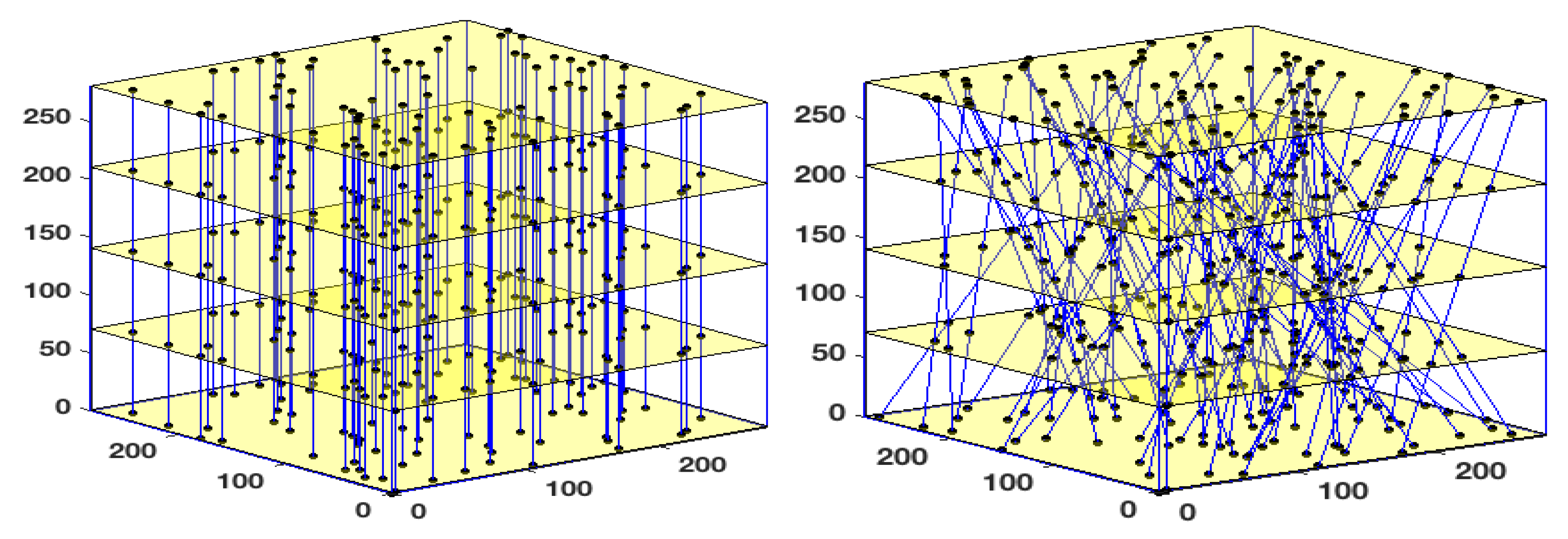
5.1. Benefits of Subsampling for OCT

The OCT imaging device, as the case of the most medical imaging systems, obeys two key requirements for successful application of compressed sensing methods: (1) medical imaging is naturally compressible by sparse coding in an appropriate transform domain (e.g., wavelet, shearlet transforms, etc.) and (2) OCT scanning system (e.g., Spectral-Domain OCT, the most used) naturally acquire encoded samples, rather than direct pixel samples (e.g., in spatial-frequency encoding). Therefore, the images resulting from Spectral-Domain OCT are sparse in native representation, hence yielding themselves well to various implementations of the ideas from Compressed Sensing theory.

Certainly, OCT enables high-speed A-scan and B-scan acquisitions (Figure 2B) but presents a serious issue when it comes to acquiring a C-scan volume. Therefore, especially in case of biological sample/tissue examination, using OCT volumes poses the problem of frame-rate acquisition (generating artifacts) as well as the data transfer i.e., several hundred Mo for each volume (Figure 2B).

Indeed, OCT volume data can be considered as a $n_1\times n_2\times n_3$ tensor of voxels. Thereby, the mathematical methods and materials related to tensors study are well suited for 3D OCT data.

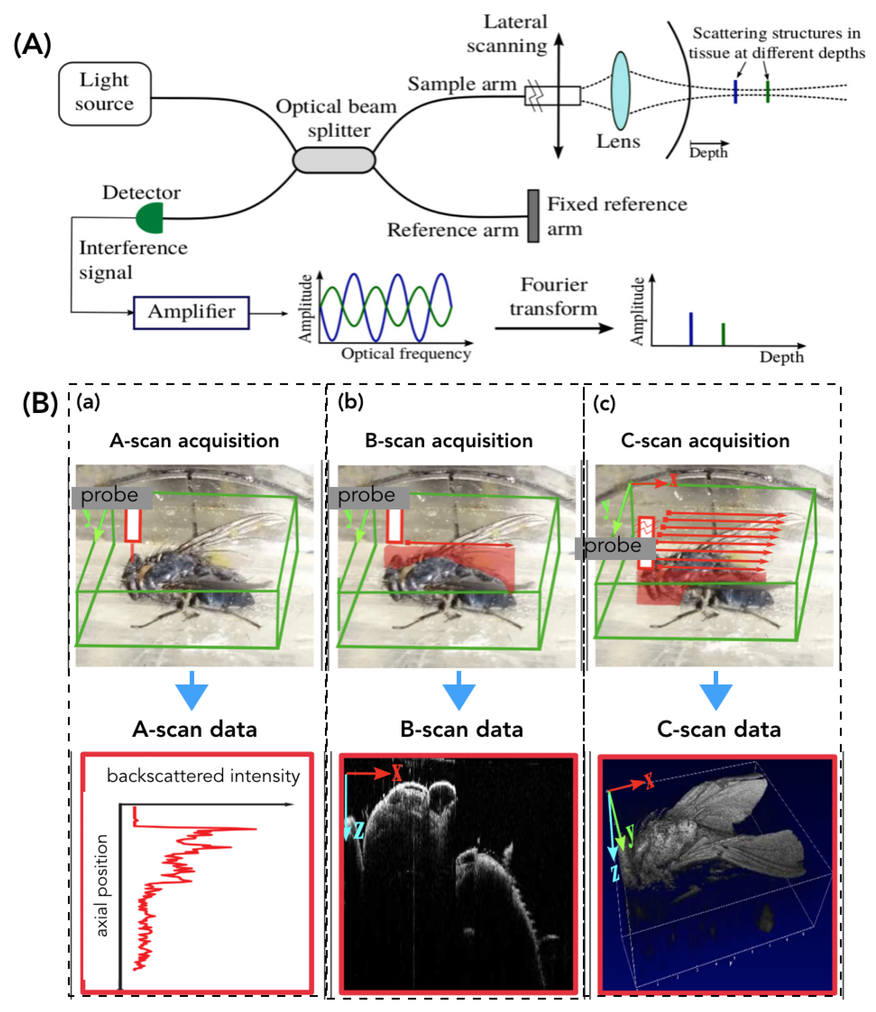
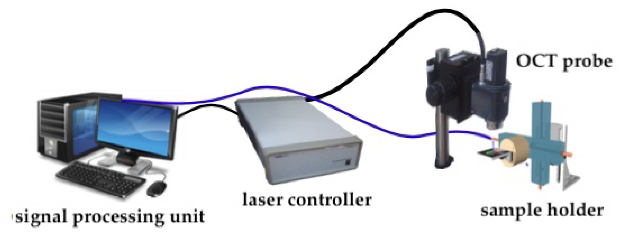
5.2. Experimental Set-Up

An OCT imaging system (Telesto-II 1325 nm spectral domain OCT) from Thorlabs (Figure 3), is used to validate the proposed distortion models. Axial (resp. lateral) resolution is 5.5 $\mathsf{\mu }$m (resp. 7 $\mathsf{\mu }$m) and up to 3.5 mm depth. The Telesto-II allows a maximum field-of-view of 10 × 10 × 3.5 mm${}^3$ with a maximum A-Scan (optical core) acquisition rate of 76 kHz.

5.3. Validation Scenario

The method proposed in this paper was implemented in a MatLab framework without taking into account the code optimization aspects as well as the time-computation. In order to validate experimentally the approach presented here, we acquired different OCT volumes (C-Scan images) of realistic biological samples: for example, a part of a grape (Figure 4 (left)) and a part of a fish eye retina (Figure 4 (right)). The size of the OCT volume used in these numerical validations, for both samples, is $A_{n\times m\times l}=281\times 281\times 281$ voxels.

To access the performance of the proposed algorithm, we constructed several undersampled 3D volume using 30%, 50%, 70%, and 90% of the original OCT volume. To do this, we created two types of 3D masks. The first consists of a pseudo-random binary masks $M_v$ using a density random sampling in which the data are selected in a vertical manner (Figure 5 (left)). For the second type of mask, instead of a vertical subsampling of the data, we designed oblique masks $M_o$ as shown in Figure 5 (right)) which are more appropriate in the case of certain imaging systems such as Magnetic Resonance Imaging (MRI), Computerized Tomography scan (CT-scan), and in certain instances, OCT imaging systems as well.

5.4. Obtained Results

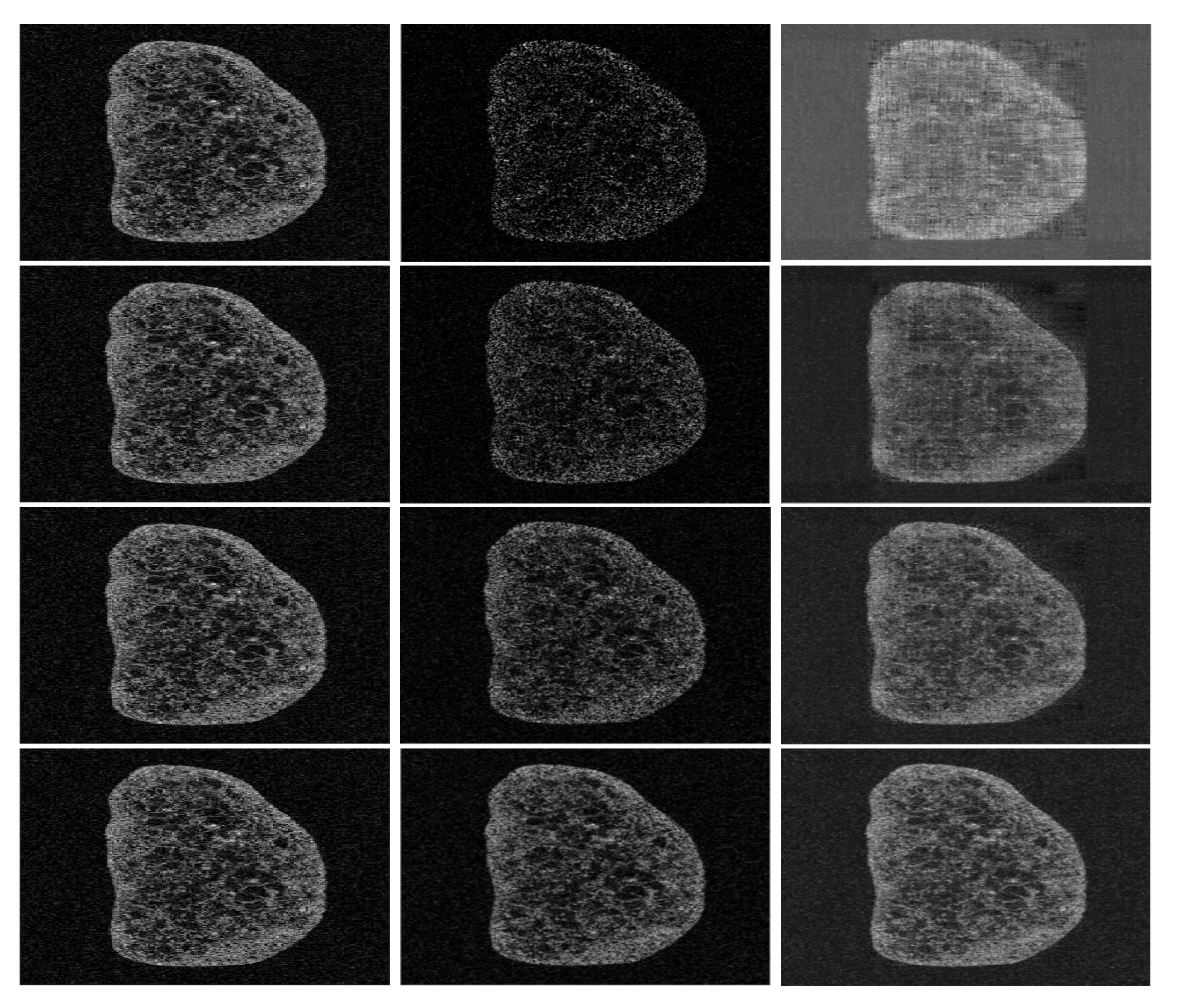
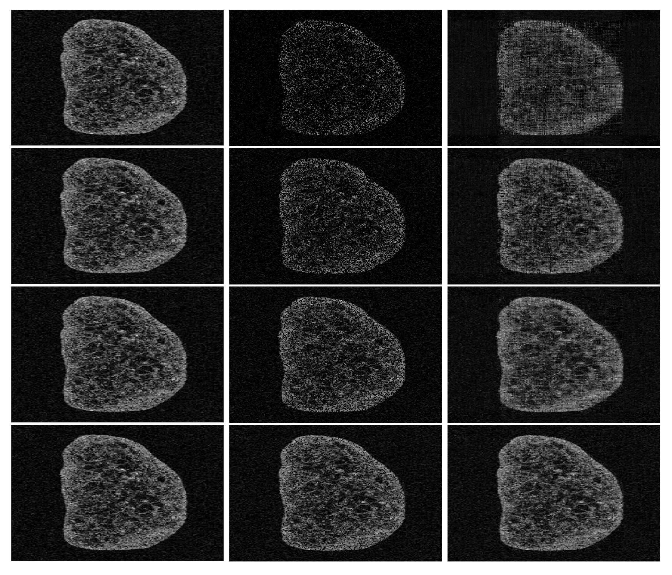
The validation scenarios were carried out as follows—the studied method was applied to each OCT volume (i.e., grape or fish eye) using various subsampling rates (i.e., 30%, 50%, 70%, and 90%). Also, in each case, the vertical $M_v$ or the oblique $M_o$ 3D binary masks were used. The results obtained with our nuclear norm penalised reconstruction approach are discussed below.

5.4.1. Grape Sample

Figure 6 and Figure 7 depict the different reconstructed OCT volumes using the oblique and the vertical binary masks. Instead of illustrating the fully reconstructed OCT volume, we choose to show 2D images (the 100th $xy$ slice of the reconstructed volumes) for a better visualization, with the naked eye, of the quality of the obtained results. It can be highlighted that the sharpness of the boundary is well preserved; however, it loses some features in the zones where the image has low intensity. This is a common effect of most of the compressed sensing and inpainting methods. In order to improve the quality of the recovered data, conventional filters based post-processing could be also be used in order to enhance contrast.

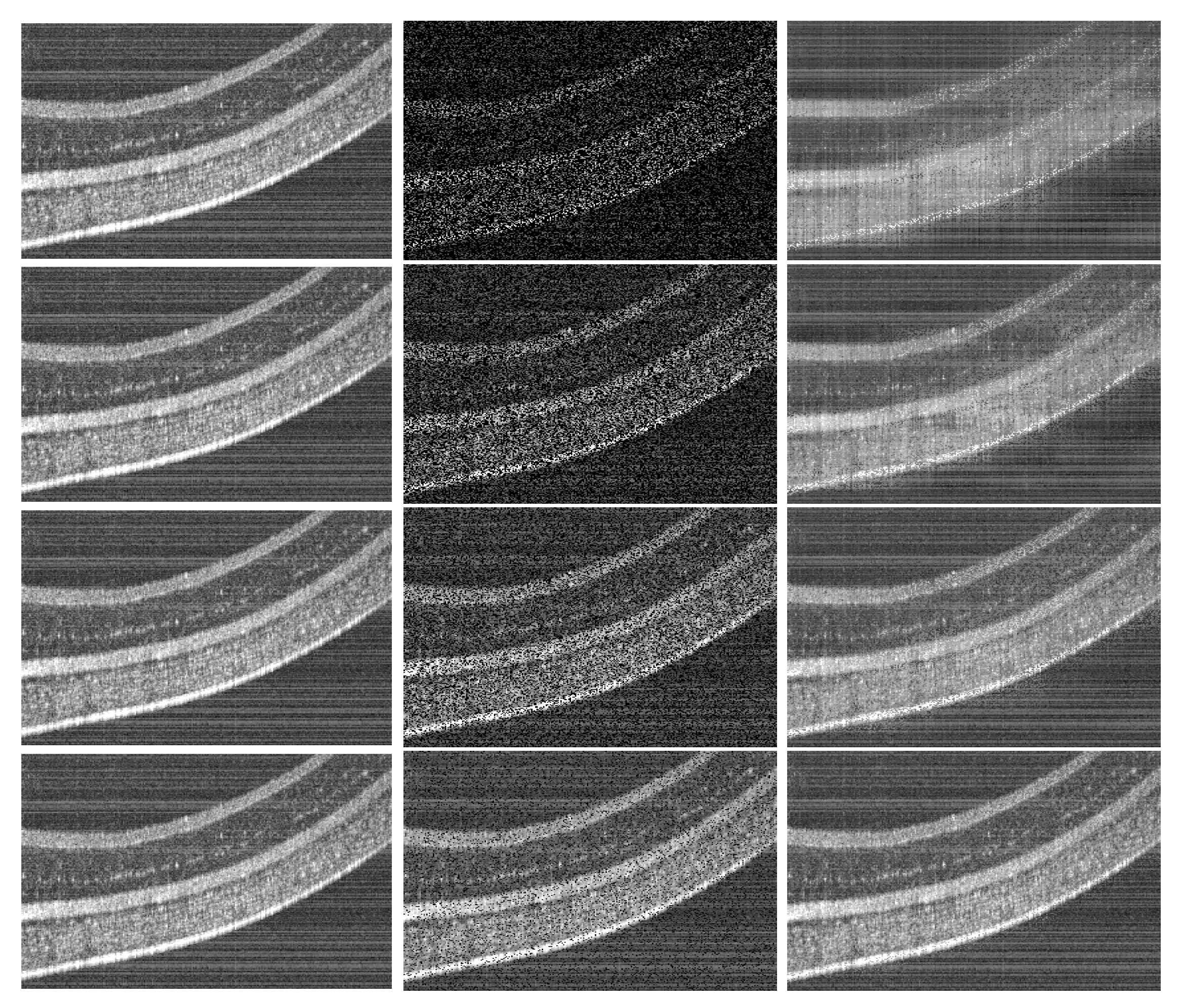
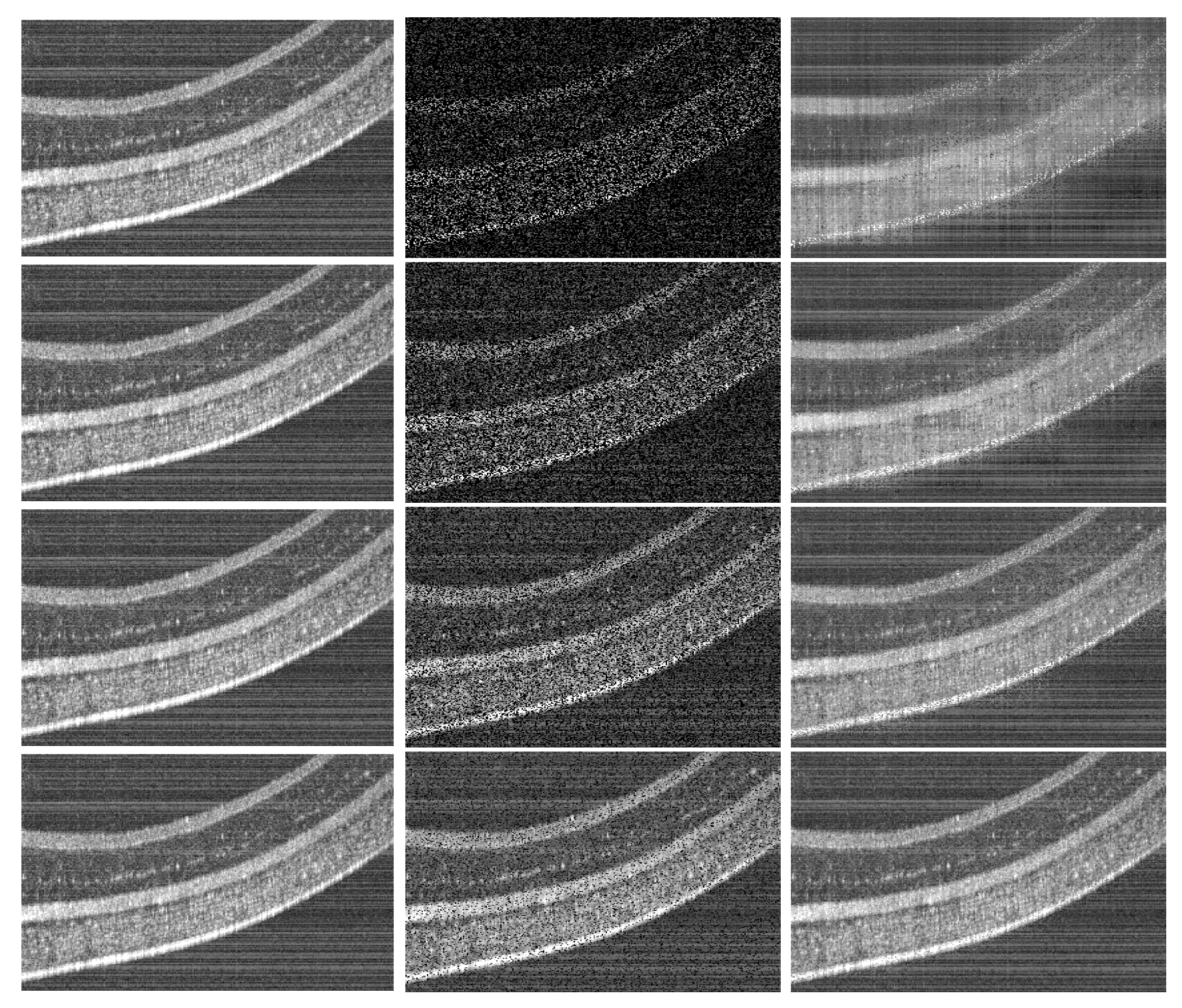
5.4.2. Fish Eye Sample

we also performed validation experiments using an optical biopsy of a fish eye (see the images sequence depicted in Figure 8 and Figure 9).

5.5. The Singular Value Thresholding Algorithm

In this section, we describe the algorithm used for the computation of our estimator, namely a tubal tensor version of the fixed point algorithm of Reference [59]. This algorithm is a very simple and scalable iterative scheme which converges to the solution of (17). Each iteration consists of two successive steps:

• a singular value thresholding step where all tubal singular values with norm below the level $2\lambda$ are set to zero and the remaining larger singular values are being removed an offset $2\lambda$.
• a relaxed gradient step.

In mathematical terms, the algorithms works as follows:

$$\begin{array}{c}\hfill \left\{\begin{array}{c}{Z}^{(l)}=shrink\left(A^{(l-1)},\delta \lambda \right)\hfill \\ A^{(l)}=A^{(l-1)}+\delta {\mathcal{P}}_{\mathsf{\Omega }}\left({\sum }_{i=1}^n{Y}_i{X}_i-Z^{(l)}\right.\hfill \end{array}\right)\end{array}$$

In the setting of our algorithm, the Shrinkage operator operates as follows:

• compute the circular Fourier transform $\mathcal{F}(A^{(l-1)})$ of the tubal components of $A^{(l-1)}$,
• compute the SVD of all the slices of $\mathcal{F}(A^{(l-1)})$ and forms the tubal singular values,
• sets to zero the tubal singular values whose ${\ell }_2$-norm lies below the level $2\delta \lambda$ and shrink the other by $2\delta \lambda$,
• recompose the spectrally thresholded matrix and take the inverse Fourier transform of the tubal components.

On the other hand, ${\mathcal{P}}_{\mathsf{\Omega }}$ is the operator that assigns to the entries indexed by $\mathsf{\Omega }$ the observed values and leaves the other values unchanged.

The convergence analysis of [59] directly applies to our setting.

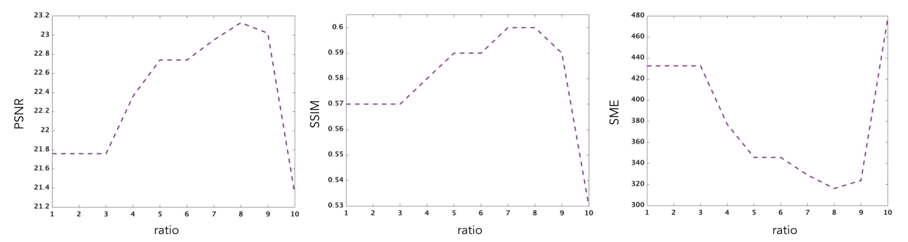
5.6. Analysis of the Numerical Results

In order to quantitatively assess the obtained results using different numerical validation scenarios and OCT images, we implemented two images similarity scores extensively employed in the image processing community. In particular, we use

• the Peak Signal Noise Ratio (PSNR) computed as follows

  $$PSNR=10{log}_{10}\left(\frac{d^2}{MSE}\right)$$

  (45)

  where d is the maximal pixel value in the initial OCT image and the $MSE$ (mean-squared error) is obtained by

  $$MSE=\sum _{i=1}^n\sum _{j=1}^m{\left(I_o(i,j)-I_r(i,j)\right)}^2$$

  (46)

  with $I_o$ and $I_r$ represent an initial 2D OCT slice (selected from the OCT volume) and the recovered one, respectively.
• The second image similarity score consists of the Structural Similarity Index (SIMM) which allows measuring the degree of similarity between two images. It is based on the computation of three values namely the luminance l, the contrast c and the structural aspect s. It is given by

  $$SSIM=(s\left(I_r,I_o)\right)(l\left(I_r,I_o\right)\left(c\left(I_r,I_o\right)\right)$$

  (47)

  where,

  $$l=\frac{2{\mu }_{I_r}{\mu }_{I_o}+C_1}{{\mu }_{I_r}^2+{\mu }_{I_o}^2+C_1},$$

  (48)

  $$c=\frac{2{\sigma }_{I_r}{\sigma }_{I_o}+C_2}{{\sigma }_{I_r}^2+{\sigma }_{I_o}^2+C_2},$$

  (49)

  $$s=\frac{2{\sigma }_{I_r,I_o}+C_3}{{\sigma }_{I_r}{\sigma }_{I_o}+C_3},$$

  (50)

  with ${\mu }_{I_r}$, ${\mu }_{I_o}$, ${\sigma }_{I_r}$, ${\sigma }_{I_o}$, and ${\mu }_{I_r,I_o}$ are the local means, standard deviations, and cross-covariance for images $I_r$, $I_o$. The variables $C_1$, $C_2$, $C_3$ are used to stabilize the division with weak denominator.

5.6.1. Illustrating the Rôle of the Nuclear Norm Penalisation

In order to understand the rôle of the nuclear norm penalisation in the reconstruction, we have performed several experiments with different values of the hyper-parameter $\lambda$ which are reported in Figure 10. This figure shows the performance of the estimator as a function of the ratio between the largest singular value and the smallest selected singular value. This ratio is an implicit function of $\lambda$, which is more intuitive than $\lambda$ for interpreting the results. The smaller the ratio, the smaller the number of singular values incorporated in the estimation.

The corresponding values are reported in

Table 1. SME, PSNR, SSIM for various values of the ratio.

Ratio	1	2	3	4	5	6	7	8	9	10
SME	432.65	432.65	432.65	377.12	345.76	345.75	329.06	316.23	323.87	477.43
PSNR	21.76	21.76	21.76	22.36	22.74	22.74	22.95	23.13	23.02	21.34
SSIM	0.57	0.57	0.57	0.58	0.59	0.59	0.60	0.60	0.59	0.53

.

The results of these experiments show that different weights for the nuclear norm penalisation imply different erros. In these experiments, one sees that the SME is optimised at a ration equal to 8 and the PSNR is maximised at 8 as well. The SSIM is maximum for values of the ratio equal to 7 and 8. Estimation which does not account for the intrinsic complexity of the object to recover will clearly fail to reconstruct the 3D images properly.

5.6.2. Performance Results

Table 2. [sample: grape]: Numerical values of the different image similarities (between initial image and reconstructed one): MSE, PSNR and SSIM.

Sample: Part of a Grape
under-sampling rates	30%	50%	70%	90%
vertical masks
MSE PSNR SSIM	536.68 20.83 0.39	316.23 23.13 0.59	185.83 25.43 0.77	62.34 30.18 0.92
oblic masks
MSE PSNR SSIM	725.20 19.52 0.34	431.91 21.77 0.55	171.52 25.78 0.78	54.85 30.73 0.93

and

Table 3. [sample: fish eye retina]: Numerical values of the different image similarities (between initial image and recontructed one): MSE, PSNR and SSIM.

Sample: Fish Eye Retina
under-sampling rates	30%	50%	70%	90%
vertical masks
MSE PSNR SSIM	829.96 18.94 000.51	570.81 20.56 0.65	333.13 22.50 0.78	109.65 27.73 0.91
oblic masks
MSE PSNR SSIM	828.56 18.94 0.51	575.90 20.52 0.65	344.12 22.76 0.77	99.13 28.16 0.92

summarise the numerical values of MSE, PSNR, SSIM computed for each test, that is, using different undersampling rates and masks, for our two different test samples (grape or fish eye retina). The parameter $\lambda$ was chosen using the simple and efficient method proposed in [60]. As expected the error decreases as a function of the percentage of observed pixels. The results also show that the estimator is not very sensitive to the orientation of the mask. There seems to be a phase transition after the 70% level, above which the reconstruction accuracy is suddenly improved in terms of PSNR and SSIM, but the method still works satisfactorily at smaller sampling rates.

6. Conclusions and Perspectives

In this paper, we studied tensor completion problems based on the framework proposed by Kilmer et al. [10]. We provided some theoretical analysis of the nuclear norm penalised estimator. These theoretical results are validated numerically using realistic OCT data (volumes) of biological samples. These encouraging results with real datasets demonstrate the relevance of the low rank assumption for practical applications. Further research will be undertaken in devising fast algorithms and incorporating other penalties such as, e.g., based on sparsity of the shearlet transform [61].

References

1. Candès, E.J. Mathematics of sparsity (and a few other things). In Proceedings of the International Congress of Mathematicians, Seoul, Korea, 13–21 August 2014. [Google Scholar]
2. Candès, E.J.; Romberg, J.; Tao, T. Robust uncertainty principles: Exact signal reconstruction from highly incomplete frequency information. IEEE Trans. Inf. Theory 2006, 52, 489–509. [Google Scholar] [CrossRef] [Green Version]
3. Recht, B.; Fazel, M.; Parrilo, P.A. Guaranteed minimum-rank solutions of linear matrix equations via nuclear norm minimization. SIAM Rev. 2010, 52, 471–501. [Google Scholar] [CrossRef] [Green Version]
4. Hackbusch, W. Tensor Spaces and Numerical Tensor Calculus; Springer Science & Business Media: Berlin, Germany, 2012; Volume 42. [Google Scholar]
5. Landsberg, J.M. Tensors: Geometry and Applications; American Mathematical Society: Providence, RI, USA, 2012; Volume 128. [Google Scholar]
6. Sacchi, M.D.; Gao, J.; Stanton, A.; Cheng, J. Tensor Factorization and its Application to Multidimensional Seismic Data Recovery. In SEG Technical Program Expanded Abstracts; Society of Exploration Geophysicists: Houston, TX, USA, 2015. [Google Scholar]
7. Yuan, M.; Zhang, C.H. On tensor completion via nuclear norm minimization. Found. Comput. Math. 2016, 16, 1031–1068. [Google Scholar] [CrossRef] [Green Version]
8. Signoretto, M.; Van de Plas, R.; De Moor, B.; Suykens, J.A. Tensor versus matrix completion: A comparison with application to spectral data. Signal Process. Lett. IEEE 2011, 18, 403–406. [Google Scholar] [CrossRef]
9. Kilmer, M.E.; Martin, C.D. Factorization strategies for third-order tensors. Linear Algebra Its Appl. 2011, 435, 641–658. [Google Scholar] [CrossRef] [Green Version]
10. Kilmer, M.E.; Braman, K.; Hao, N.; Hoover, R.C. Third-order tensors as operators on matrices: A theoretical and computational framework with applications in imaging. SIAM J. Matrix Anal. Appl. 2013, 34, 148–172. [Google Scholar] [CrossRef] [Green Version]
11. Koltchinskii, V.; Lounici, K.; Tsybakov, A.B. Nuclear-norm penalization and optimal rates for noisy low-rank matrix completion. Ann. Stat. 2011, 39, 2302–2329. [Google Scholar] [CrossRef]
12. Candes, E.J.; Plan, Y. Matrix completion with noise. Proc. IEEE 2010, 98, 925–936. [Google Scholar] [CrossRef] [Green Version]
13. Anandkumar, A.; Ge, R.; Hsu, D.; Kakade, S.M.; Telgarsky, M. Tensor decompositions for learning latent variable models. J. Mach. Learn. Res. 2014, 15, 2773–2832. [Google Scholar]
14. Signoretto, M.; Dinh, Q.T.; De Lathauwer, L.; Suykens, J.A. Learning with tensors: A framework based on convex optimization and spectral regularization. Mach. Learn. 2014, 94, 303–351. [Google Scholar] [CrossRef] [Green Version]
15. So, A.M.C.; Ye, Y. Theory of semidefinite programming for sensor network localization. Math. Program. 2007, 109, 367–384. [Google Scholar] [CrossRef]
16. Eriksson, B.; Balzano, L.; Nowak, R. High-rank matrix completion and subspace clustering with missing data. arXiv 2011, arXiv:1112.5629. [Google Scholar]
17. Candès, E.J.; Recht, B. Exact matrix completion via convex optimization. Found. Comput. Math. 2009, 9, 717–772. [Google Scholar] [CrossRef] [Green Version]
18. Singer, A.; Cucuringu, M. Uniqueness of low-rank matrix completion by rigidity theory. SIAM J. Matrix Anal. Appl. 2010, 31, 1621–1641. [Google Scholar] [CrossRef] [Green Version]
19. Fazel, M. Matrix Rank Minimization with Applications. Ph.D. Thesis, Stanford University, Stanford, CA, USA, 2002. [Google Scholar]
20. Gross, D. Recovering low-rank matrices from few coefficients in any basis. Inf. Theory IEEE Trans. 2011, 57, 1548–1566. [Google Scholar] [CrossRef] [Green Version]
21. Recht, B. A simpler approach to matrix completion. J. Mach. Learn. Res. 2011, 12, 3413–3430. [Google Scholar]
22. Candès, E.J.; Tao, T. The power of convex relaxation: Near-optimal matrix completion. Inf. Theory IEEE Trans. 2010, 56, 2053–2080. [Google Scholar] [CrossRef] [Green Version]
23. Kolda, T.G.; Bader, B.W. Tensor decompositions and applications. SIAM Rev. 2009, 51, 455–500. [Google Scholar] [CrossRef]
24. McCullagh, P. Tensor Methods in Statistics; Chapman and Hall: London, UK, 1987; Volume 161. [Google Scholar]
25. Rogers, M.; Li, L.; Russell, S.J. Multilinear Dynamical Systems for Tensor Time Series. Adv. Neural Inf. Process. Syst. 2013, 26, 2634–2642. [Google Scholar]
26. Ge, R.; Huang, Q.; Kakade, S.M. Learning mixtures of gaussians in high dimensions. arXiv 2015, arXiv:1503.00424. [Google Scholar]
27. Mossel, E.; Roch, S. Learning nonsingular phylogenies and hidden Markov models. In Proceedings of the Thirty-Seventh Annual ACM Symposium on Theory of Computing, Baltimore, MD, USA, 22–24 May 2005; pp. 366–375. [Google Scholar]
28. Jennrich, R. A generalization of the multidimensional scaling model of Carroll and Chang. UCLA Work. Pap. Phon. 1972, 22, 45–47. [Google Scholar]
29. Kroonenberg, P.M.; De Leeuw, J. Principal component analysis of three-mode data by means of alternating least squares algorithms. Psychometrika 1980, 45, 69–97. [Google Scholar] [CrossRef]
30. Bhaskara, A.; Charikar, M.; Moitra, A.; Vijayaraghavan, A. Smoothed analysis of tensor decompositions. In Proceedings of the 46th Annual ACM Symposium on Theory of Computing, New York, NY, USA, 1–3 June 2014; pp. 594–603. [Google Scholar]
31. De Lathauwer, L.; De Moor, B.; Vandewalle, J. A multilinear singular value decomposition. SIAM J. Matrix Anal. Appl. 2000, 21, 1253–1278. [Google Scholar] [CrossRef] [Green Version]
32. Kolda, T.G. Symmetric Orthogonal Tensor Decomposition is Trivial. arXiv 2015, arXiv:1503.01375. [Google Scholar]
33. Robeva, E.; Seigal, A. Singular Vectors of Orthogonally Decomposable Tensors. arXiv 2016, arXiv:1603.09004. [Google Scholar] [CrossRef] [Green Version]
34. Hao, N.; Kilmer, M.E.; Braman, K.; Hoover, R.C. Facial recognition using tensor-tensor decompositions. SIAM J. Imaging Sci. 2013, 6, 437–463. [Google Scholar] [CrossRef]
35. Semerci, O.; Hao, N.; Kilmer, M.E.; Miller, E.L. Tensor-based formulation and nuclear norm regularization for multienergy computed tomography. Image Process. IEEE Trans. 2014, 23, 1678–1693. [Google Scholar] [CrossRef] [Green Version]
36. Zhang, Z.; Aeron, S. Exact tensor completion using t-svd. IEEE Trans. Signal Process. 2017, 65, 1511–1526. [Google Scholar] [CrossRef]
37. Pothier, J.; Girson, J.; Aeron, S. An algorithm for online tensor prediction. arXiv 2015, arXiv:1507.07974. [Google Scholar]
38. Tibshirani, R. Regression shrinkage and selection via the lasso. J. R. Stat. Soc. Ser. Methodol. 1996, 58, 267–288. [Google Scholar] [CrossRef]
39. Bickel, P.J.; Ritov, Y.; Tsybakov, A.B. Simultaneous analysis of Lasso and Dantzig selector. Ann. Stat. 2009, 37, 1705–1732. [Google Scholar] [CrossRef]
40. Candès, E.J.; Plan, Y. Near-ideal model selection by l1 minimization. Ann. Stat. 2009, 37, 2145–2177. [Google Scholar] [CrossRef]
41. Zou, H. The adaptive lasso and its oracle properties. J. Am. Stat. Assoc. 2006, 101, 1418–1429. [Google Scholar] [CrossRef] [Green Version]
42. Zou, H.; Hastie, T. Regularization and variable selection via the elastic net. J. R. Stat. Soc. Ser. Stat. Methodol. 2005, 67, 301–320. [Google Scholar] [CrossRef] [Green Version]
43. Gaïffas, S.; Lecué, G. Weighted algorithms for compressed sensing and matrix completion. arXiv 2011, arXiv:1107.1638. [Google Scholar]
44. Xu, Y. On Higher-order Singular Value Decomposition from Incomplete Data. arXiv 2014, arXiv:1411.4324. [Google Scholar]
45. Raskutti, G.; Yuan, M. Convex Regularization for High-Dimensional Tensor Regression. arXiv 2015, arXiv:1512.01215. [Google Scholar] [CrossRef] [Green Version]
46. Barak, B.; Moitra, A. Noisy Tensor Completion via the Sum-of-Squares Hierarchy. arXiv 2015, arXiv:1501.06521. [Google Scholar]
47. Gandy, S.; Recht, B.; Yamada, I. Tensor completion and low-n-rank tensor recovery via convex optimization. Inverse Probl. 2011, 27, 025010. [Google Scholar] [CrossRef] [Green Version]
48. Mu, C.; Huang, B.; Wright, J.; Goldfarb, D. Square Deal: Lower Bounds and Improved Convex Relaxations for Tensor Recovery. In Proceedings of the International Conference on Machine Learning, Beijing, China, 21–26 June 2014. [Google Scholar]
49. Amelunxen, D.; Lotz, M.; McCoy, M.B.; Tropp, J.A. Living on the edge: Phase transitions in convex programs with random data. Inf. Inference 2014, 3, 224–294. [Google Scholar] [CrossRef]
50. Lecué, G.; Mendelson, S. Regularization and the small-ball method I: Sparse recovery. arXiv 2016, arXiv:1601.05584. [Google Scholar] [CrossRef] [Green Version]
51. Watson, G.A. Characterization of the subdifferential of some matrix norms. Linear Algebra Its Appl. 1992, 170, 33–45. [Google Scholar] [CrossRef] [Green Version]
52. Lewis, A.S. The convex analysis of unitarily invariant matrix functions. J. Convex Anal. 1995, 2, 173–183. [Google Scholar]
53. Hu, S. Relations of the nuclear norm of a tensor and its matrix flattenings. Linear Algebra Its Appl. 2015, 478, 188–199. [Google Scholar] [CrossRef]
54. Chrétien, S.; Wei, T. Von Neumann’s inequality for tensors. arXiv 2015, arXiv:1502.01616. [Google Scholar]
55. Chrétien, S.; Wei, T. On the subdifferential of symmetric convex functions of the spectrum for symmetric and orthogonally decomposable tensors. Linear Algebra Its Appl. 2018, 542, 84–100. [Google Scholar] [CrossRef] [Green Version]
56. Heinze, H.; Bauschke, P.L. Convex Analysis and Monotone Operator Theory in Hilbert Spaces; Canada Mathematical Society: Ottawa, ON, Canada, 2011. [Google Scholar]
57. Borwein, J.; Lewis, A.S. Convex Analysis and Nonlinear Optimization: Theory and Examples; Springer Science & Business Media: Berlin, Germany, 2010. [Google Scholar]
58. Jean-Pierre Aubin, I.E. Applied Nonlinear Analysis; Dover Publications: Mineola, NY, USA, 2006; Volume 518. [Google Scholar]
59. Ma, S.; Goldfarb, D.; Chen, L. Fixed point and Bregman iterative methods for matrix rank minimization. Math. Program. 2011, 128, 321–353. [Google Scholar] [CrossRef]
60. Chrétien, S.; Lohvithee, M.; Sun, W.; Soleimani, M. Efficient hyper-parameter selection in Total Variation- penalised XCT reconstruction using Freund and Shapire’s Hedge approach. Mathematics 2020, 8, 493. [Google Scholar] [CrossRef] [Green Version]
61. Guo, W.; Qin, J.; Yin, W. A new detail-preserving regularization scheme. SIAM J. Imaging Sci. 2014, 7, 1309–1334. [Google Scholar] [CrossRef]
62. Tropp, J.A. User-Frindly tail bounds for sums of random matrices. arXiv 2010, arXiv:1004.4389v7. [Google Scholar]
Figure 1. The t-SVD of a tensor.
Mathematics 08 00628 g001
Figure 2. Illustration of the Fourier-Domain Optical Coherence Tomography (OCT) operating. (A) the optical principle and (B) the different available acquisition modes: A-scan (1D optical core), B-Scan (2D image), and C-scan (volume).
Mathematics 08 00628 g002
Figure 3. Global view of the OCT acquisition setup.
Mathematics 08 00628 g003
Figure 4. Examples of the OCT volumes of biological samples used to validate the proposed method. (first row) the initial OCT volumes and (second row), B-scan images (100th vertical slice) taken from the initial volumes.
Mathematics 08 00628 g004
Figure 5. Illustration of the implemented 3D masks used to subsampled the data and creating the 3D masks. (Left) a 3D mask allowing a vertical and random selection of the data, and (right) a 3D mask allowing an oblique selection of the subsampled data.
Mathematics 08 00628 g005
Figure 6. [sample: grape, mask: vertical]—Reconstructed OCT images (only a 2D slice is shown in this example). Each row corresponds to an under-sampling rate: 30% (1st row), 50% (2nd row), 70% (3th row), and 90% (4th row). The first column represents the initial OCT image, the second column the under-sampled data used for the reconstruction, and the third column, the recovered OCT images.
Mathematics 08 00628 g006
Figure 7. [sample: grape, mask: oblic]—Reconstructed OCT images (only a 2D slice is shown in this example). Each row corresponds to an under-sampling rate: 30% (1st row), 50% (2nd row), 70% (3th row), and 90% (4th row). The first column represents the initial OCT image, the second column the under-sampled data used for the reconstruction, and the third column, the recovered OCT images.
Mathematics 08 00628 g007
Figure 8. [sample: fish eye retina, mask: vertical]—Reconstructed OCT images (only a 2D slice is shown in this example). Each row corresponds to an under-sampling rate: 30% (1st row), 50% (2nd row), 70% (3th row), and 90% (4th row). The first column represents the initial OCT image, the second column the under-sampled data used for the reconstruction, and the third column, the recovered OCT images.
Mathematics 08 00628 g008
Figure 9. [sample: fish eye retina, mask: oblic]—Reconstructed OCT images (only a 2D slice is shown in this example). Each line corresponds to an under-sampling rate: 30% (1st line), 50% (2nd line), 70% (3th line), and 90% (4th line). The first column represents the initial OCT image, the second column the under-sampled data used for the reconstruction, and the third column, the recovered OCT images.
Mathematics 08 00628 g009
Figure 10. Evolution of the PSNR, SSIM and SME performance criteria as a function of the ratio between the largest singular value and the smallest singular value selected by the penalised estimator.
Mathematics 08 00628 g010