Gas–Liquid Two-Phase Flow Investigation of Side Channel Pump: An Application of MUSIG Model

Abstract

This paper introduces a novel application of a multiphase flow model called the Multi-Size-Group model (MUSIG) to solve 3D complex flow equations in a side channel pump, in order to analyze the flow dynamics of the gas phase distribution and migration under different inlet gas volume fractions (IGVFs). Under different IGVF, the suction side is more likely to concentrate bubbles, especially near the inner radius of the impeller, while there is very little or no gas at the outer radius of the impeller. The diameter of bubbles in the impeller are similar and small for most regions even at IGVF = 6% due to the strong shear turbulence flow which eliminates large bubbles. Additionally, this method also can capture the coalescence and breakage evolution of bubbles. Once a mixture of fluid goes into the impeller from the inlet pipe, the large bubbles immediately break, which accounts for the reason why nearly all side channel pumps have the capacity to deliver gas–liquid two-phase flow. The results in this study provide a foundation and theoretical value for the optimal design of side channel pumps under gas–liquid two-phase conditions to increase their application.

1. Introduction

As a kind of regenerative pump, side channel pumps seem appropriate and economical for industrial application due to their unique operational characteristic advantages, such as high head generation, multiphase flow, self-priming capabilities, and transportation of hot and volatile fluids. They are widely used in manufacturing processes due to their ability to deliver liquid–gas two-phase flow with air fraction up to 50%, compared to the 25% of some centrifugal pumps [1]. Thus, these pumps have great potential in the biomedical, petrochemical, chemical, and food processing fields. However, the flow inside a side channel pump attains a screw-like pathway after several movements between the radial impeller and the side channel as shown in Figure 1 [2]. There are many vortexes in different directions in the flow of side channel pumps. When gas is added, the internal flow in side channel pump becomes more unsteady [3]. Thus, it is a challenge to research two-phase flow characteristics due to the extremely complex inner flows exhibited.

The concept of side channel pumps was first proposed in 1920, with the first model pump utilized for community water supply [4]. With modification of geometrical parameters, side channel pumps evolved to transporting both viscous liquids and gases. Further studies were performed on the effects of different geometrical parameters (shape, length, and width of blade and side channel) on the hydraulic performance of side channel pumps through numerical simulations and experiments [5,6,7,8,9,10]. However, these studies considered only pure water as the fluid material, neglecting the excellent two-phase transport ability of the pumps. Recently, experimental studies have investigated the performance of a side channel pump using three types of blades with different suction angles under gas–liquid two-phase flow operating conditions [3]. In addition, the acoustic and vibrational effects of the two-phase liquid–gas flow characteristics were compared with the results from a single-phase flow in side channel pumps. This confirmed that an additional gas out hole can promote phase separation, which leads to a better two-phase flow handling of the pump [11]. However, these studies only compared the hydraulic performances between pure water and liquid–gas two-phase flow, neglecting the study of the internal flow characteristics.

Early studies of the multiphase flow of vane pumps were mainly conducted via experiments [12,13]. Visualization experiments were conducted on an electric submersible pump (ESP) through high-speed photography, and the gas–liquid flow was divided into bubble flow, agglomerated bubble flow, gas pocket flow, and segregated flow. It was found that the hydraulic performance of the pump is mainly related to the orientations of bubble flow [14]. The double fluid model was first used in pumps, and the results of experiment and numerical calculation were similar; this suggests the double fluid model has the capacity to predict the performance of a two-phase (non-condensable) flow pump [15]. Moreover, one-dimensional and two-fluid models which consider fluid viscosity and air compressibility were applied to two-phase flow pumps. The models assumed both phases have the same streamlines and the slip velocity between the two phases takes place only in the direction of the streamlines [16]. Through comparison with experiments, it was found that the method was suitable for low specific speed (n_s = 23.55) radial flow centrifugal pumps. The geometrical shape, change of medium density, and gas–liquid separation was taken into consideration, as well as compression and condensation of the gas phase, and an improved model was eventually proposed to predict the performance of a pump in the gas–liquid phase [17]. The Euler–Euler fluid model is the commonest mathematical algorithm used to numerically simulate the flow of hydraulic pumps, which can possibly reveal the internal flow patterns [18,19,20]. In addition, a systematic study of the internal energy conversion of a centrifugal pump has been conducted, and the research results provide a basis for improving the performance of single- and multi-phase centrifugal pumps, which is of great value for engineering applications [21]. However, due to the extreme complexity of the internal flow characteristics of side channel pumps, the common gas–liquid two-phase models, including the double Euler heterogeneous flow model, cannot predict the multi-vortex, multi-bubble, and multi-directional flow, especially when the gas phase is introduced. Thus, there is a need to introduce a novel and advanced mathematical model to solve the 3D complex two-phase flows in side channel pumps.

This paper therefore introduces for the first time a model for the gas–liquid two-phase simulation calculation of low specific speed (n_s < 12) pumps. The Multi-Size-Group (MUSIG) model considers discrete phase bubbles of different diameters, neglecting the assumption of traditional uniform discrete phases (which assumes all bubbles are of the same diameter and shape). The concept of a homogeneous MUSIG model was proposed in 1995 and implemented into CFX 5.7 [22]. A large number of in-depth studies of bubble coalescence and breakup in vertical pipes verified the reliability of the MUSIG model [23,24,25,26,27]. Further investigations were focused on the theoretical models and mechanisms of the MUSIG model [28,29,30]. Presently, the MUSIG model is commonly used in the field of chemical heterogeneous reactions and flow boilers [31,32,33]. However, the application of the MUSIG model in two-phase transport flow in hydraulic pumps has not been explored.

To study the internal flow characteristics of multi-stage side channel pumps under gas–liquid two-phase flow, the single-stage side channel pump with radial impeller was selected as the physical model in this work. Firstly, numerical simulations were used to analyze the internal flow characteristics in the side channel pump under a mixture of gas and liquid transport via the MUSIG model in order to acquire the flow dynamics of the gas phase distribution and migration under different inlet gas volume fractions (IGVFs). Furthermore, the coalescence and breakage evolution of bubbles in the single-stage pump was studied in detail. The results supplied in this study provide a new standpoint to investigate the flow dynamics of gas–liquid two-phase flow patterns in other vaned pumps.

2. Numerical Model and Simulation

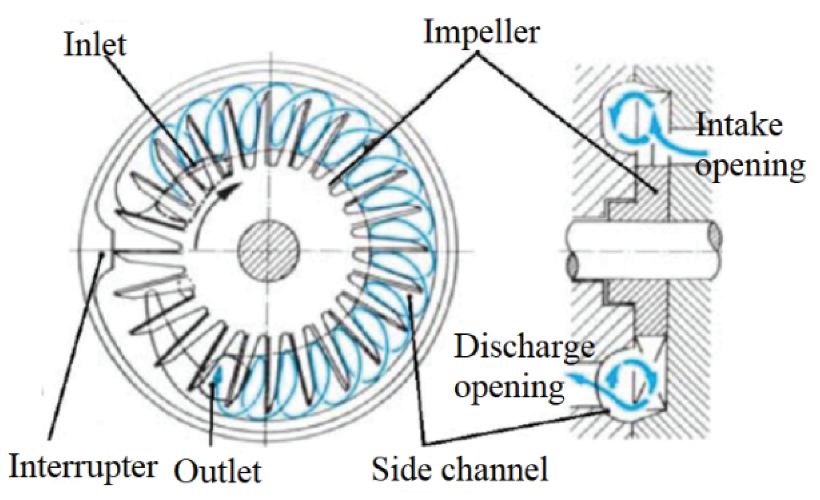
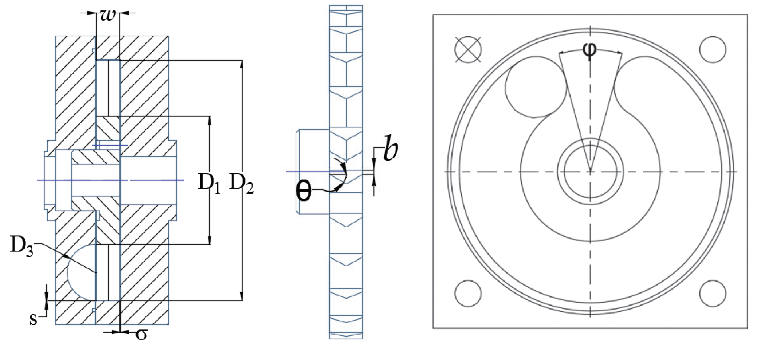
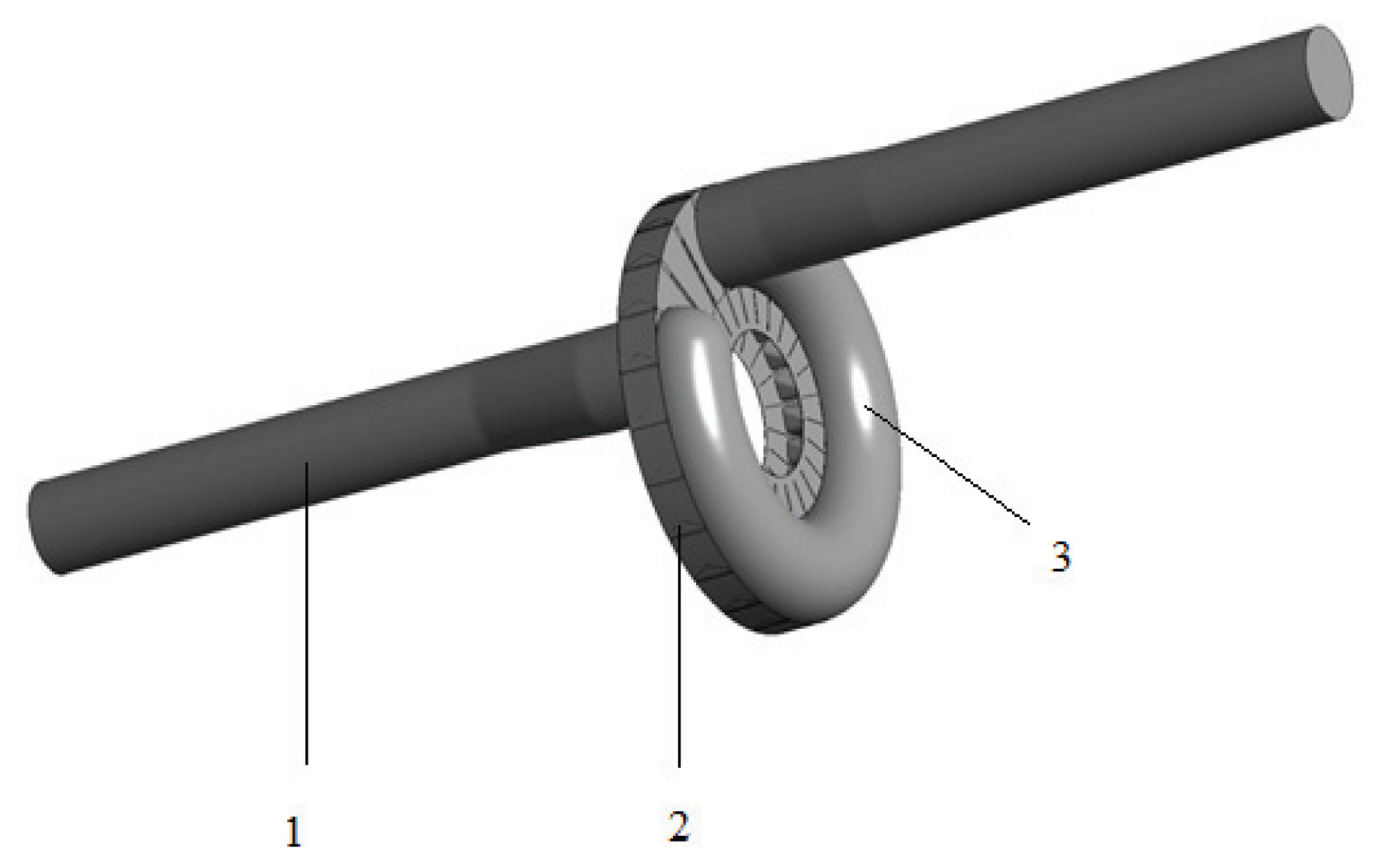
2.1. Pump Model

The side channel pump comprises two main components, namely, the impeller and side channel. Figure 2 shows the 2D structure of the investigated impeller and side channel. The detailed design parameters and global pump geometry can be found in the literature [34]. In addition, the specific speed (n_s = nQ^0.5/H^0.75) of the studied pump model is 11.2, the design flow rate and rotating speed are 10 m³/h and 1500 r/min, respectively, while the designed head is 13.5 m. The impeller consists of 24 blades with suction angle 30° and the wrapping angle of the side channel is 30°. The 3D computational flow domains of the investigated side channel model were generated using NX modeling software and divided into three (inlet, impeller, and side channel with outlet) as depicted in Figure 3. The radial and axial gaps were merged to the impeller flow domain, and the side channel and outlet pipe were also merged. This was done to reduce the number of interfaces and improve the accuracy of the simulation.

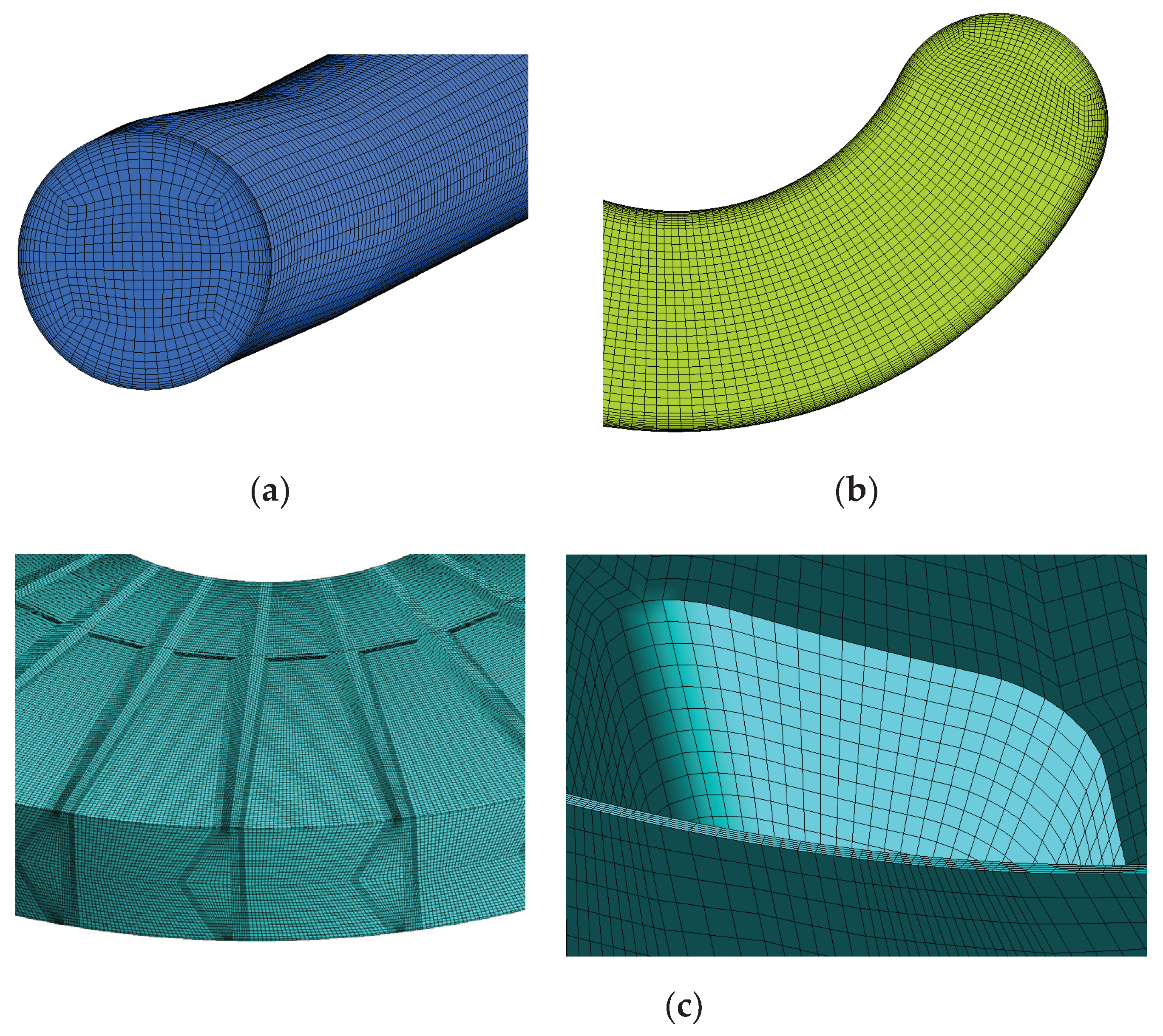
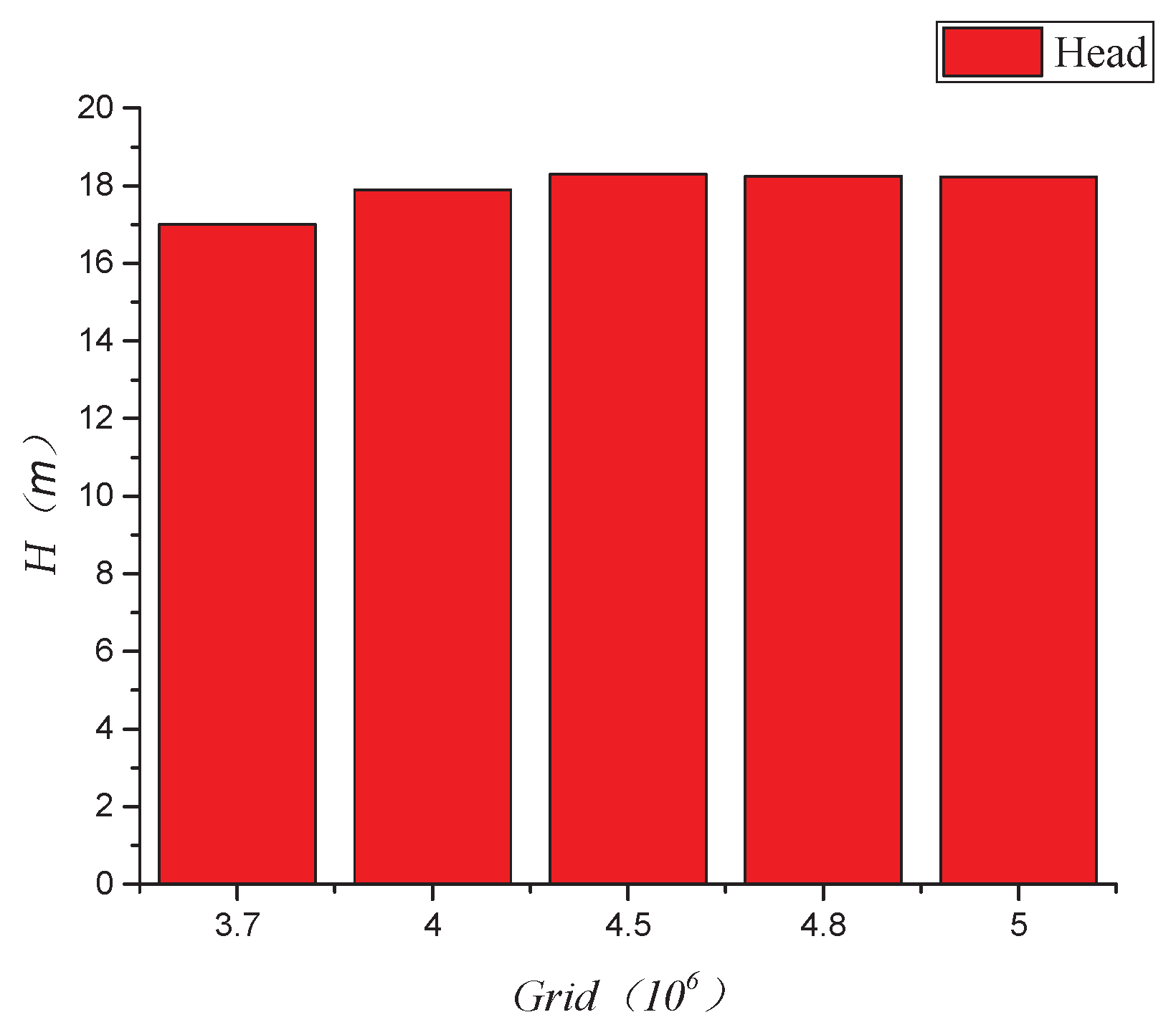
2.2. Boundary Setting and Mesh Independence

ANSYS ICEM commercial software was used to mesh the 3D computational flow domains generated. The domains were meshed using the structured blocking hexahedral method due to the flexibility of mesh quality control, and the boundary layer mesh refinement. Figure 4 shows the mesh topology of the flow domains. ANSYS CFX was used for calculation; here, the static pressure was imposed on the inlet section while the velocity based on the mass flow rate was assigned on the outlet section. The steady simulation was calculated for 1000 iterations as the initiation of transient calculation. Then, the relative position between the impeller and side channel was updated at each timestep, which had the values 1.11 × 10⁻⁴ s for the whole 5 rotations, equivalent to the time interval required for the impeller to rotate 1°. To ensure the computational accuracy, mesh independence analysis was conducted at the design flow rate of Q =10 m³/h for pure water state under rotating speed n = 1500 r/min. As shown in Figure 5, the head became relatively stable after increasing the grid number to 4.5 million elements. In addition, Figure 6 reveals the velocity streamlines in the middle plane of the impeller under different mesh numbers. The complex flows leading to minimal differences were still observed among the vortexes deduced from streamlines and, vice versa, the vortex filled in the impeller under different directions may also increase the uncertainty of the changes in the velocity streamlines. However, the intensity and general distribution of the vortexes at the middle section and the region close to the inlet were very similar after increasing the grid number to 4.5 million. At the middle section, the vortex mainly concentrates in the corner at the outer radius, and there are more fluent streamlines in these passages than other places. The extremely serious vortexes exist in the area near the inlet region. The high intensity vortex always appears in the same place in this part after increasing the grid number to 4.5 million, which confirms the general flow law is stable. Based on the procedures and methods for estimating discretization error in CFD applications [35], the mesh of 4.5 million elements was selected for further calculations. The hydraulic pump characteristic curve at different volumetric flows under pure water was checked in the previous literature [34,36].

Table 1. Structured grid data.

Domain	Grid Number (×106)	Grid Quality Criterion				Average Yplus
		Determinant 3 × 3 × 3	Angle (°)	Aspect Ratio	Mesh Size (mm)
Inlet	0.1	0.60–1	46.89–89.64	1.27–40.1	0.01–1.5	18.54
Impeller	3.4	0.62–1	20.62–87.91	1.10–23.0	0.01–0.8	34.28
Side channel	1.0	0.57–1	37.78–89.90	1.28–42.4	0.01–1.5	43.94

gives detailed information of the structured mesh used [34,36].

2.3. Turbulence Model

This study adopts the SST k-ω turbulence model [9,37], which was developed by [38,39]. It is a combination of the k-ε and the k-ω equations. The k-ω equations are used to calculate flows around the inner boundary layers. The equations switch to k-ε equations which are extremely sensitive to the free-shear layers. Therefore, k-ε equations are modified into k-ω equations with blending functions. In a wide range of fields, SST k-ω is independent of the k-ε and has high convergence accuracy in near-wall free flow. For the above reason, the SST k-ω model is a mixed model widely used in engineering.

SST k-ω equations are as follows:

$$\frac{\partial (\rho k)}{\partial t}+\frac{\partial }{\partial x_j}(\rho U_{j}k)=\frac{\partial }{\partial x_j}\left[\left(\mu +\frac{{\mu }_t}{{\sigma }_{k1}}\right)\frac{\partial k}{\partial x_j}\right]+P_k-{\beta }^{\prime }\rho k\omega$$

(1)

$$\frac{\partial (\rho \omega )}{\partial t}+\frac{\partial }{\partial x_j}(\rho U_j\omega )=\frac{\partial }{\partial x_j}\left[\left(\mu +\frac{{\mu }_t}{{\sigma }_{\omega 1}}\right)\frac{\partial \omega }{\partial x_j}\right]+{\alpha }_1\frac{\omega }{k}{P}_k-{\beta }_1\rho {\omega }^2$$

(2)

The k-ω equation for the inner boundary layer prediction is applied using the following coefficients: σ_k1 = 1.176, σ_ω1 = 2.0, β₁ = 0.075, α₁ = 5/9, β’ = 0.09 [40].

2.4. MUSIG Model

The starting point for the MUSIG model is the population balance equation. Let n (m, t) represent the number density of particles of mass m at time t. Thus, the population balance equation is given as [40]:

$$\frac{\partial }{\partial t}n\left(m,t\right)+\frac{\partial }{\partial x^i}\left(U^i\left(m,t\right)n\left(m,t\right)\right)=B_B-D_B+B_C-D_C$$

(3)

where B_B, D_B, B_C, and D_C, respectively, represent the birth rate due to breakdown of larger particles, the death rate due to breakdown into smaller particles, the birth rate due to coalescence of smaller particles, and the death rate due to coalescence with other particles. These rates may further be expressed as:

$$B_B={\displaystyle \underset{m}{\overset{\infty }{\int }}g\left(\varsigma ;m\right)}n\left(\varsigma ,t\right)d\varsigma$$

(4)

$$D_B=n\left(m,t\right){\displaystyle \underset{0}{\overset{\infty }{\int }}g\left(m;\varsigma \right)}d\varsigma$$

(5)

$$B_C=\frac{1}{2}{\displaystyle \underset{0}{\overset{m}{\int }}Q\left(m-\varsigma ;\varsigma \right)}n\left(m-\varsigma ,t\right)n\left(m,t\right)d\varsigma$$

(6)

$$D_C=n\left(m,t\right){\displaystyle \underset{0}{\overset{\infty }{\int }}Q\left(m;\varsigma \right)}n\left(\varsigma ,t\right)dt$$

(7)

where g (m; ς) represents the specific breakdown rate (the rate at which particles of mass m break into particles of mass ς and m – ς) and Q (m; ς) represents the specific coalescence rate (the rate at which particles of mass m coalesce with particles of mass ς to form particles of mass m + ς).

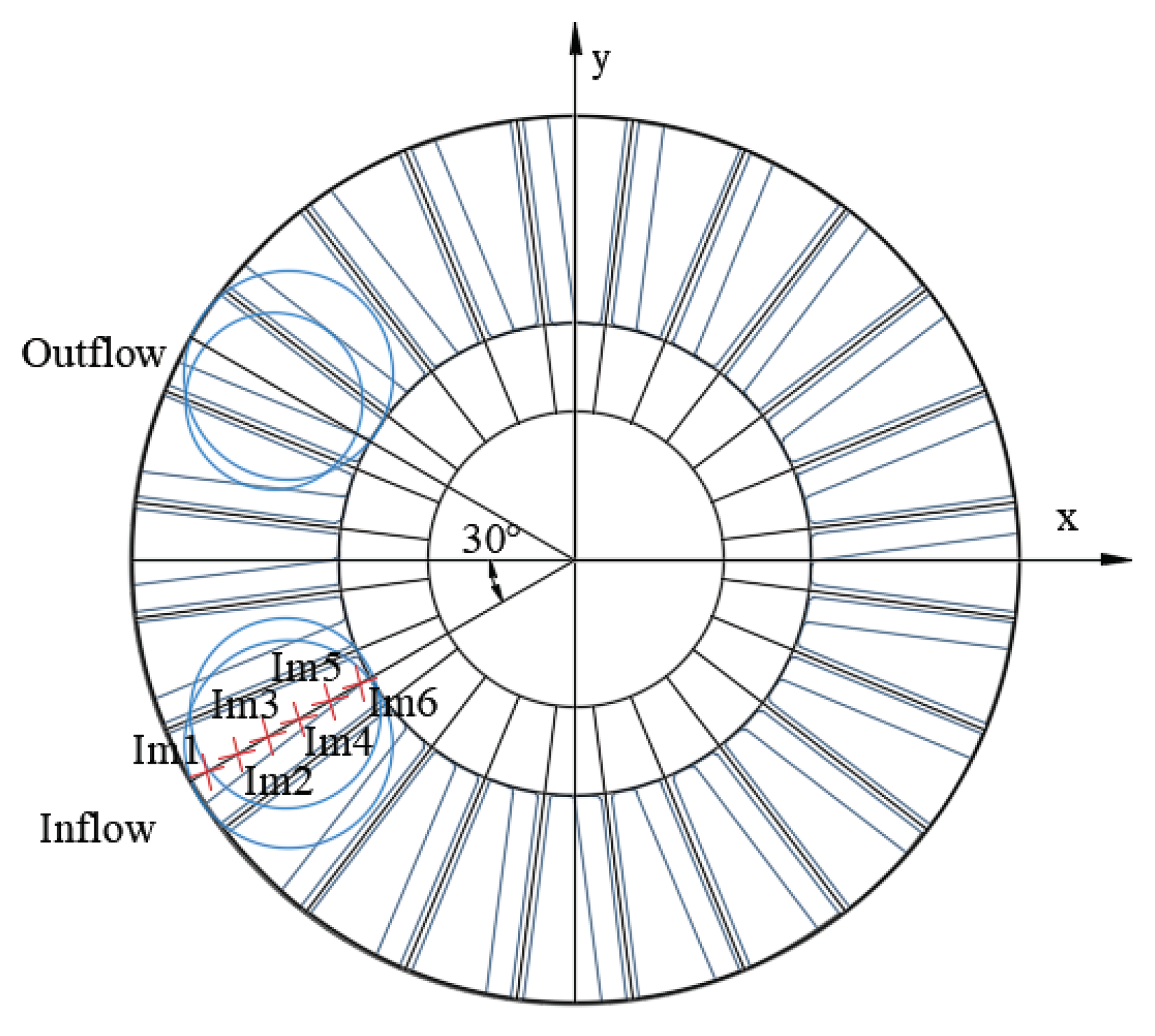
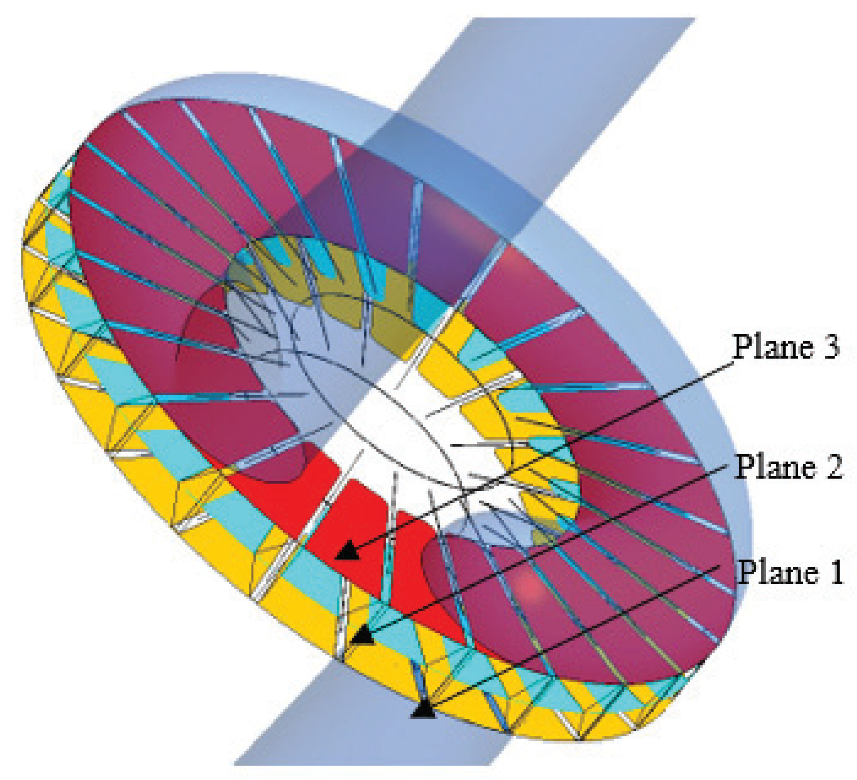
2.5. Monitoring Points

The GVF and diameters of bubbles were monitored in the impeller at different positions as indicated in Figure 7. Six monitoring points were set to 6 mm apart from the inner radius, 42 mm to outer radius, and 72 mm to obtain the detailed flow behavior. The starting positions of these monitoring points are in the impeller passage corresponding to the inlet region. The gas data in the impeller passage were recorded at z = 7.5 mm where the fluid patterns are highly disordered [34]. The specific positions of these points are provided in

Table 2. Position of monitoring points.

Point	Impeller	x (mm)	y (mm)	z (mm)
1	IM1	−36	−62.35	7.5
2	IM2	−33	−57.16	7.5
3	IM3	−30	−51.96	7.5
4	IM4	−27	−46.77	7.5
5	IM5	−24	−41.57	7.5
6	IM6	−21	−36.37	7.5

.

3. Experimental Pump Performance Characteristics

3.1. Experimental Apparatus

The hydraulic performance experiment under gas–liquid two-phase flow was conducted at the Technical University of Kaiserslautern, Germany. The experimental measurements were carried out using a closed loop to isolate uncontrollable air outside from contacting water in the tank directly. This is done to ensure the accuracy of the IGVF. The main parts of the test rig in Figure 8 are a tank with volume 2500 L for water supply, pipes to deliver mixture fluid, and data acquisition system for investigation.

In order to obtain a clear visualization of inner flow behavior, the pump casing was made with plexiglass, while the impeller was manufactured with aluminum to ensure blade strength. A variable speed AC motor (7AA112M04) from ELEKTRA Company was used to control the shaft of the pump, and the range of the frequency converter matching with the motor was from 0 Hz to 50 Hz corresponding to rotating speed from 0 r/min to 1500 r/min. Two pressure sensors with uncertainty of 0.15% and measuring range of 0–10 bar were installed at the inlet and outlet pipes to record pressure data. The electromagnetic flowmeter, to monitor volumetric flow rate in real time, was manufactured by Endress+Hauser Company, and has a range of 0.9–30 m³/h and maximum measuring error of ±0.5%. Furthermore, a gas injection device was installed at the inlet pipe to the gas medium. A gas mass flow controller with measuring error of only ±0.3% (Bürkert Company, Ingelfingen, Germany) was installed in the gas injection pipe to control the gas inflow. The software LabVIEW 8.5 was used to record 20 data samples for each opening of the valve for further data processing.

To ensure accuracy and reliability, all data was collected twice under each operating condition. In addition, the random uncertainty of the experimental measurement under the pure water state was carried out with a 95% confidence probability. The random uncertainty of flow rate, head, rotational speed, torque, and power were ±0.08%, ±0.24%, ±0.01%, ±0.17%, and ±0.17%, respectively.

3.2. Experimental Validation with the MUSIG

The dimensionless coefficient flow rate Φ and head coefficient ψ were evaluated using Equations (8) and (9). Moreover, the IGVF Ω was defined by Equation (10) to express the inlet gas volume fraction.

$$\mathsf{\Phi }=\frac{4·\left(Q_g+Q_l\right)}{\pi ·d^2·u_2}$$

(8)

$$\psi =\frac{\Delta p_{tot}}{\frac{1}{2}·\rho ·{u_2}^2}$$

(9)

$$\mathsf{\Omega }=\frac{Q_g}{Q_g+Q_l}$$

(10)

where Q_l is flow rate of the liquid, m³/h; Q_g is flow rate of the gas, L/min.

Figure 9 shows the hydraulic performance under single phase, IGVF = 2%, 4%, and 6%. Here, a drop in the head coefficient is observed with increasing IGVF and the curves representing the working condition are also shortened. However, compared with the tendency of falling sharply under single phase, the downward trend is slow and may even rise slightly under two-phase. Comparatively, the side channel pump is highly sensitive to gas.

It can be seen from Figure 10 that under the condition of ventilation, the simulated value is slightly larger than the experimental value. The overall simulation trend is similar to the experimental results. The head gradually decreases and, particularly when the IGVF increases from 2% to 6%, the head decreases gradually. However, the experimental head rapidly decreases when the IGVF increases from 0% to 2%, which falls much faster than the CFD head. The first reason is that the vortex is one of the main causes of pump cavitation [41], and as a special type of pump, there are a lot of vortexes in the side channel pump in different directions, resulting in easy cavitation of side channel pumps. The second reason is that the cavitation performance of low specific speed pumps drops sharply under gas–liquid two-phase flow. The larger the IGVF, the lower the cavitation performance [42]. Due to the poor cavitation resistance of the side channel pump, cavitation may occur when ventilating only a small amount of air; this is why the experimental value is lower than the simulation value under the condition of gas–liquid mixed transport. Nonetheless, the comparison still shows that the MUSIG model is suitable for the simulation of the mixture of gas and liquid in the side channel pump without cavitation.

4. Results and Discussion

4.1. Head Fluctuation

Figure 11 depicts the head fluctuation coefficients of gas–liquid two-phase flow under different IGVF. The head coefficient, ψ, is plotted on the y-axis and the timestep of the impeller rotation is plotted on the x-axis. The timestep is measured in rotating degrees. The side channel pump revealed 24 regular head fluctuations under low IGVF, which is equal to the blade number. Pei [36] reported similar results after investigating the same pump model under single phase, and Pei [43] also investigated unsteady flow performance in centrifugal pump, the fluctuation in the centrifugal pump is much lower than in the side channel pump. Thus, the dataset that corresponds to the maximum point were subjected to further detailed analyses. The peak of head fluctuation under single phase is about 3.2 times higher than two-phase. In an overall view, the head coefficient fluctuates more fiercely in a whole circle under high IGVF. With the increase of IGVF, the hydraulic head of the pump also has an obvious decline.

4.2. Analysis on the Internal Flow Characteristics

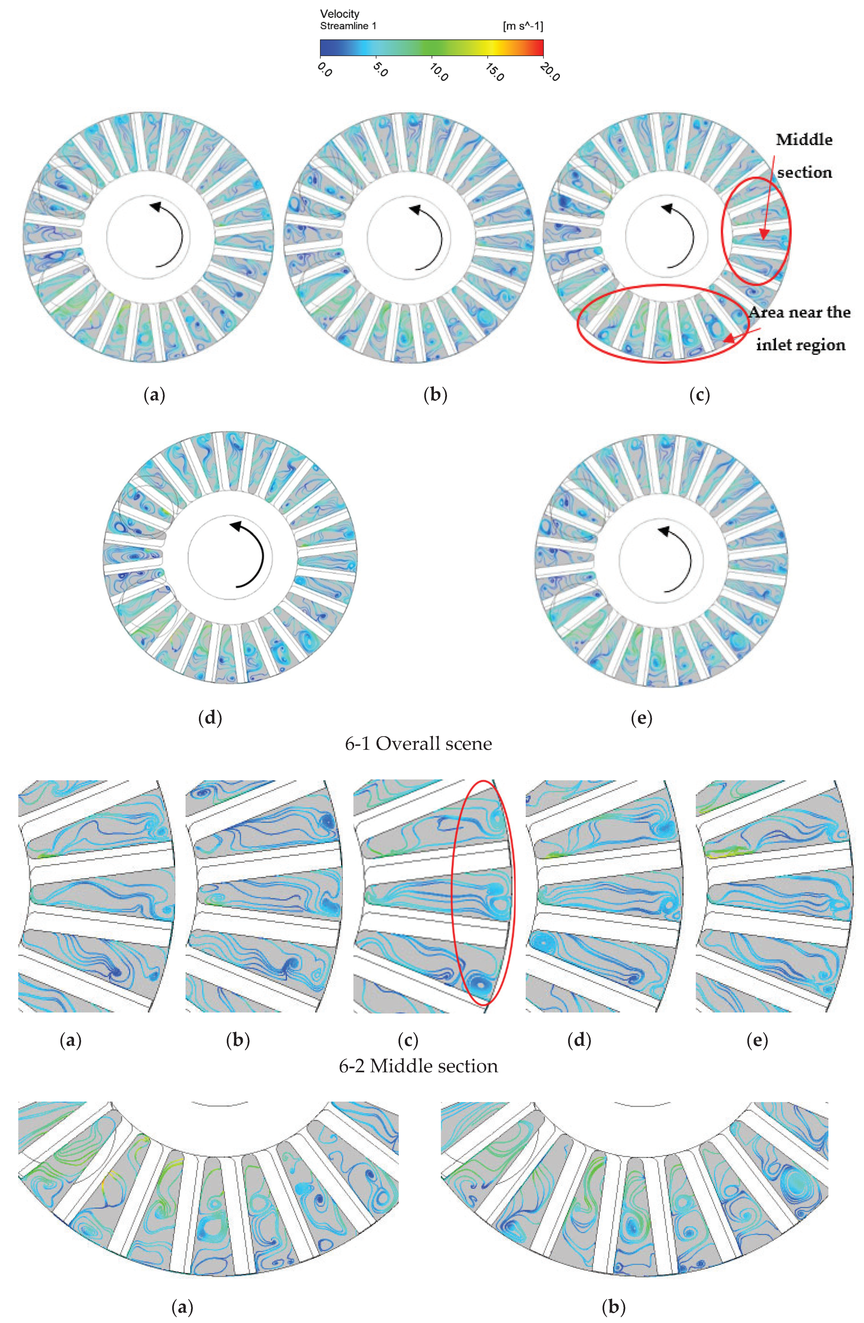
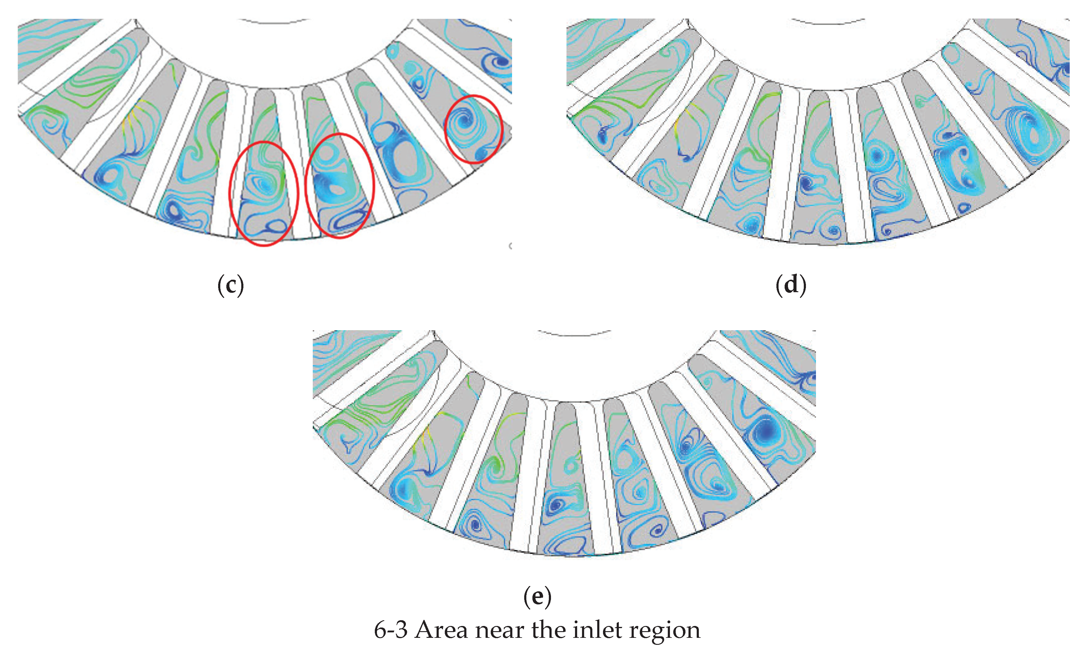
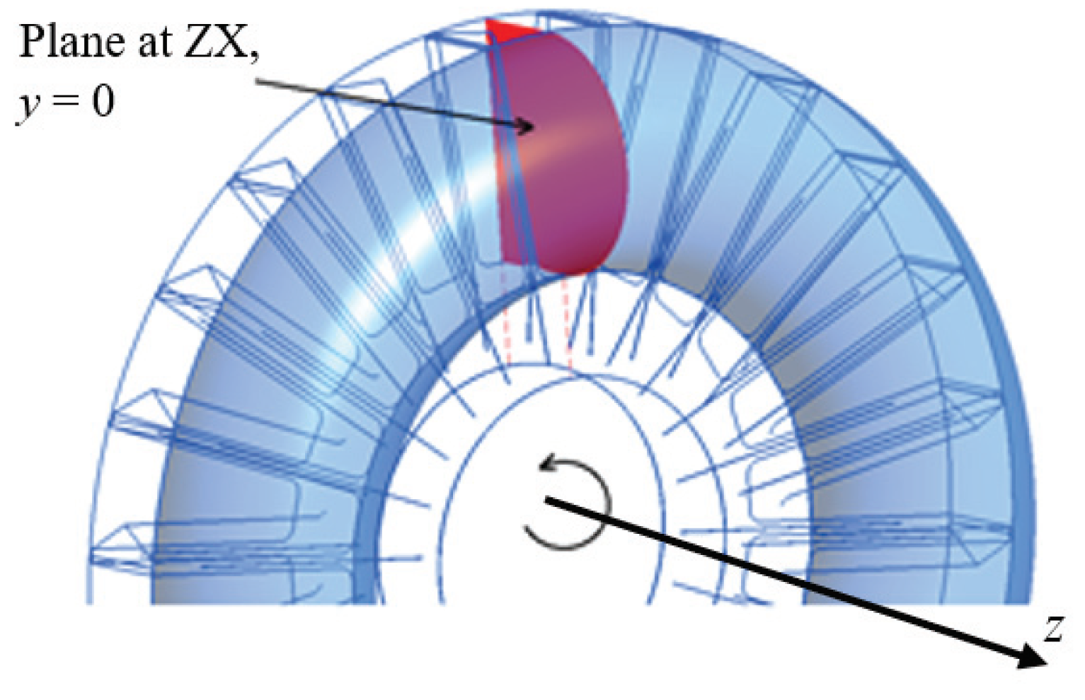
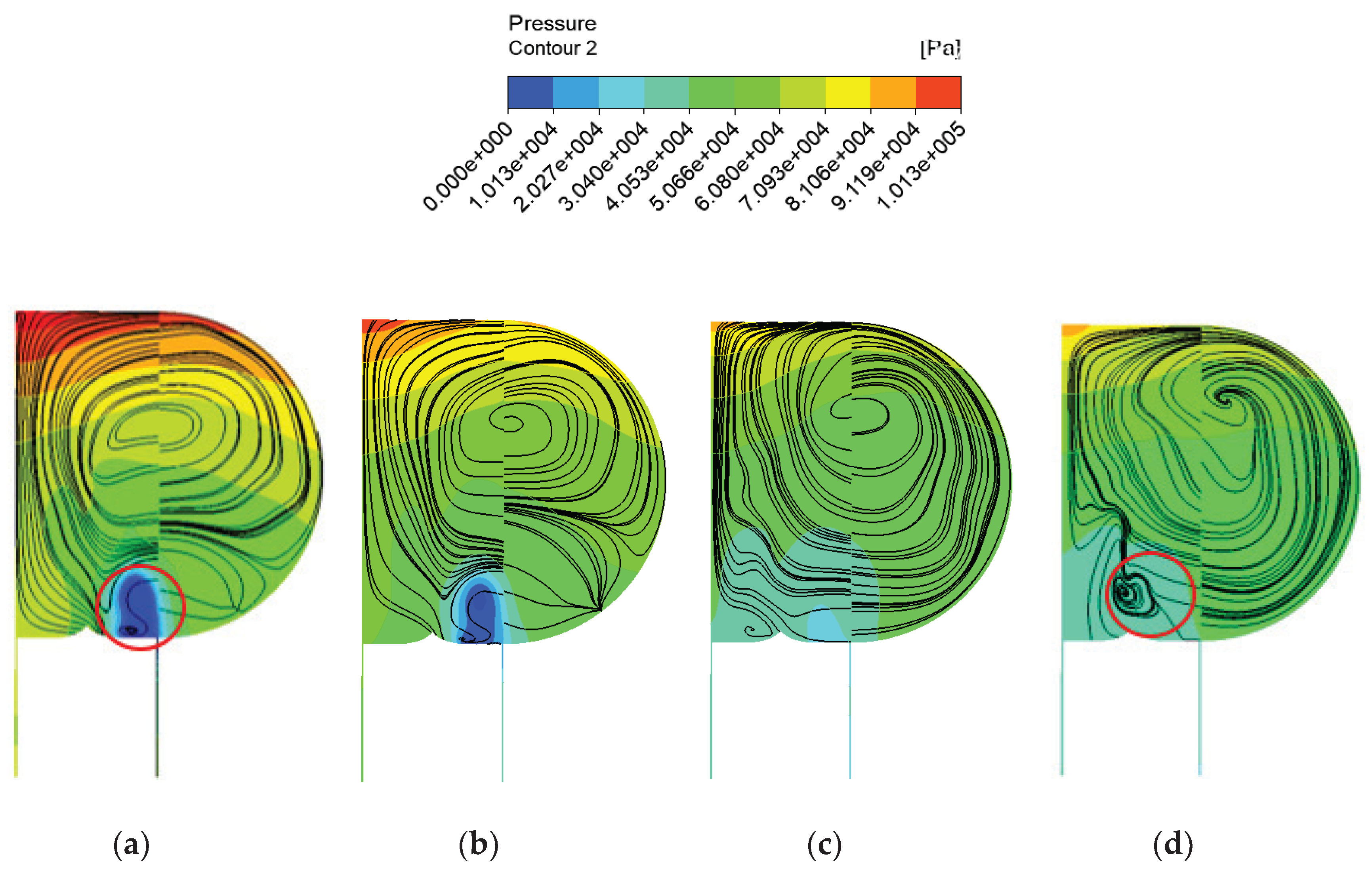
4.2.1. Pressure and Velocity Analysis

Figure 12 shows the static pressure distribution coupled with velocity streamlines of single phase (pure water) and two-phase flow under IGVF 2%, IGVF 4% and IGVF 6% on the side channel wall at the maximum point. From an overview, there is a vortex near 150° offset from the inflow at all operating conditions. This can be attributed to the sudden change in design of the side channel [44]. From inlet to outlet, the pressure gradient rises, and the pressure of the outer radius rises about 5 × 10⁴ pa faster than the inner radius at the same rotation angle in the side channel. The rotating fluid flows out from the outer radius of the blade into the stationary side channel and travels into the inner part of the next blade. The increased rate of pressure under single phase becomes much larger than under two-phase. Part A at the middle section of the side channel typically records an area of obvious vortex, which means big flow loss. Firstly, when fluid flows into the side channel at the inlet region, the force to make the fluid rotate back to the impeller is low, leading to weak axial velocity. However, the radial velocity is based on the rotational speed, and is relatively higher than the axial velocity at the initial position. Thus, after about 11 blade movements, the streamlines are continuous, from the outer radius on the boundary near the inlet, to the inner radius on the boundary at part A near the middle section. With the force increasing, the axial velocity also increases and the streamlines can finish the cycle across just 4 or 5 blades. Part A is an area where the velocity and pressure both have significant change leading to the appearance of the typical vortex. Comparing Figure 12b to Figure 12a, the proportion and degree of turbulent flow increases. There is also a difference under IGVF 2%: the mixture fluid will have a decrease in velocity and pressure which may delay the significant change, leading to the main vortex moving from part A to B. Then, after increasing IGVF to 4% and 6%, the main vortex moves from part B to C. This shows that ventilation has a great influence on the vortex in the middle section of the side channel pump, but the overall streamline patterns are similar to those under single phase.

Figure 13 is a plane set on the zx axis at y = 0. This plane corresponds to part A in Figure 12 where the vortex exists on the side channel surface. Figure 14 shows the pressure distribution and velocity streamlines on the plane as shown in Figure 13. It shows that under low IGVF, the pressure contour is similar. From the inner radius to the outer radius, the pressure gradient grows in a similar manner to that on the side channel wall. With the single-phase pure water condition, there is a very low-pressure region with slightly deformed velocity streamlines in the impeller near the inner radius. Under IGVF 2%, the low-pressure region still exists, but the small vortex has disappeared. Due to the strong vortex near the middle section, the rotate streamlines are divided into two parts. When the IGVF increases from 2% to 4%, the structures of pressure and velocity streamline contours change remarkably due to the main vortex movement. Although the pressure behavior satisfies the law of gradient growth from inner radius to outer radius, the obvious low-pressure region disappears. Generally, the pressure is much lower than in the single phase. Finally, after increasing IGVF from 4% to 6%, the pressure is similar to IGVF 4%, but a new vortex is created with strong intensity at the inner radius of the impeller. Then, under IGVF = 6%, it is important to note that a tiny vortex also appears at the central radius of the impeller, which is likely due to the poor fluid exchange between the impeller and side channel.

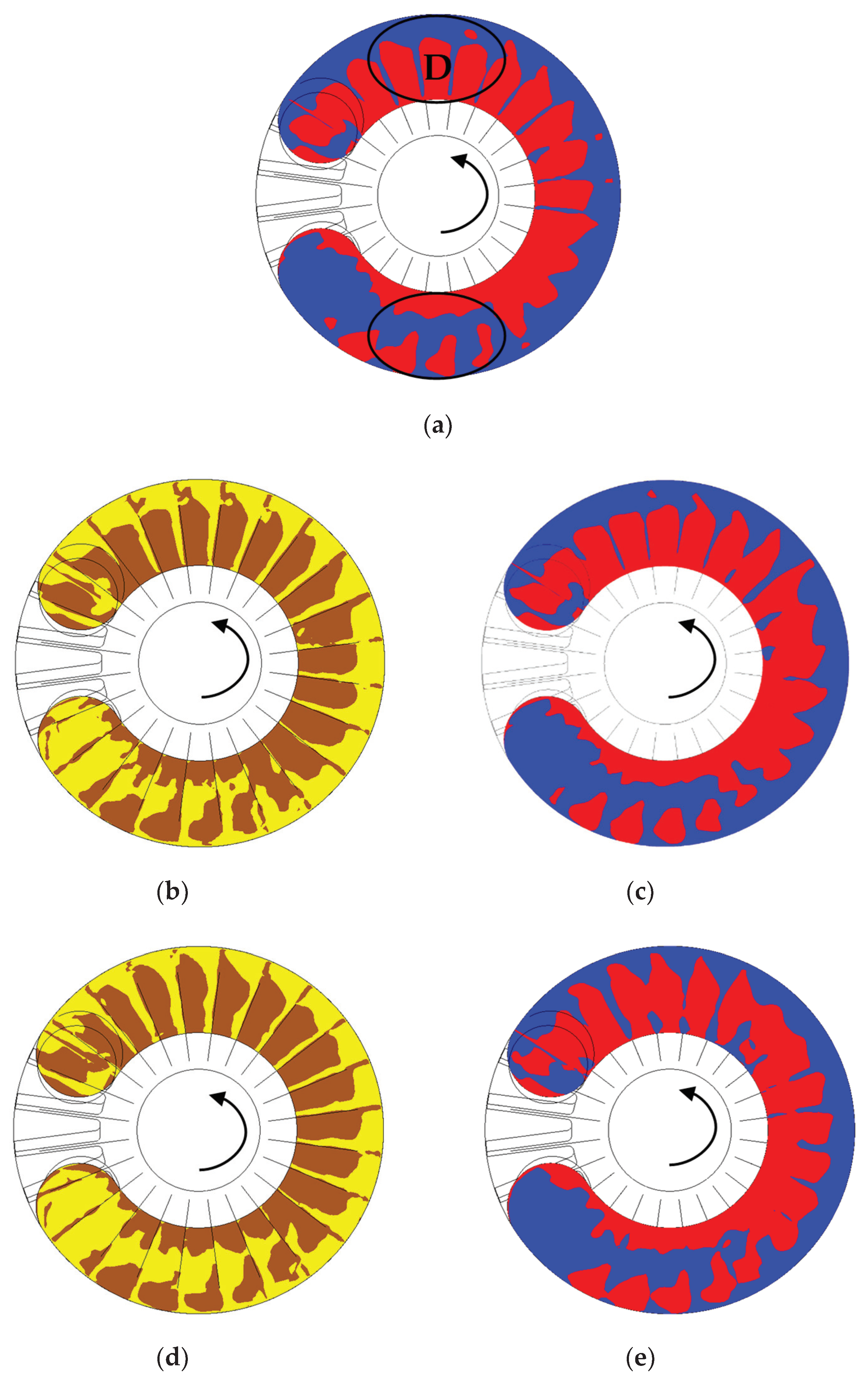
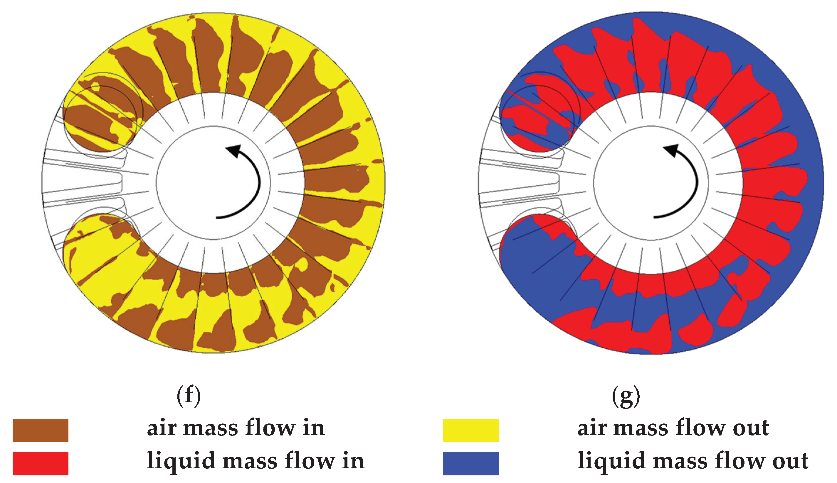
4.2.2. Exchanged Mass Flow

Figure 15 shows the exchanged mass flow distribution between the impeller and side channel in the xy plane at z =15.21 mm. Here, the blue color region represents the fluid flowing into the impeller while the red represents the fluid flowing out of the impeller into the side channel. The distribution of air phase and liquid phase under different IGVFs is similar at the inlet region. This can be associated with the sudden change in the side channel geometry. The flow exchange view shows that the fluid that flows out of the side channel mainly exists near the inner radius of the impeller. After the impeller rotates about 30° from the inlet region, the outer radius also appears at area D where mass flows in, then gradually approaches the inner radius and merges into a large area where fluid flows into impeller, approximately in the range of 0–0.7 D₂. However, the exchanged mass flow near the outlet region shows little difference. As the IGVF increases, the area where mass flows in extends closer to the outer radius and even connects. Comparing the air phase to the liquid phase, the gas moves in the liquid, thus the distribution law of the exchange mass flow of gas is similar to that of the liquid. However, with increasing IGVF, the area of the gas flowing into the impeller close to the outflow region is significantly larger than that of the liquid. Furthermore, there is also a very narrow area at the outer radius of each blade for the gas flowing into the impeller.

4.3. Gas Distribution in Side Channel Pump

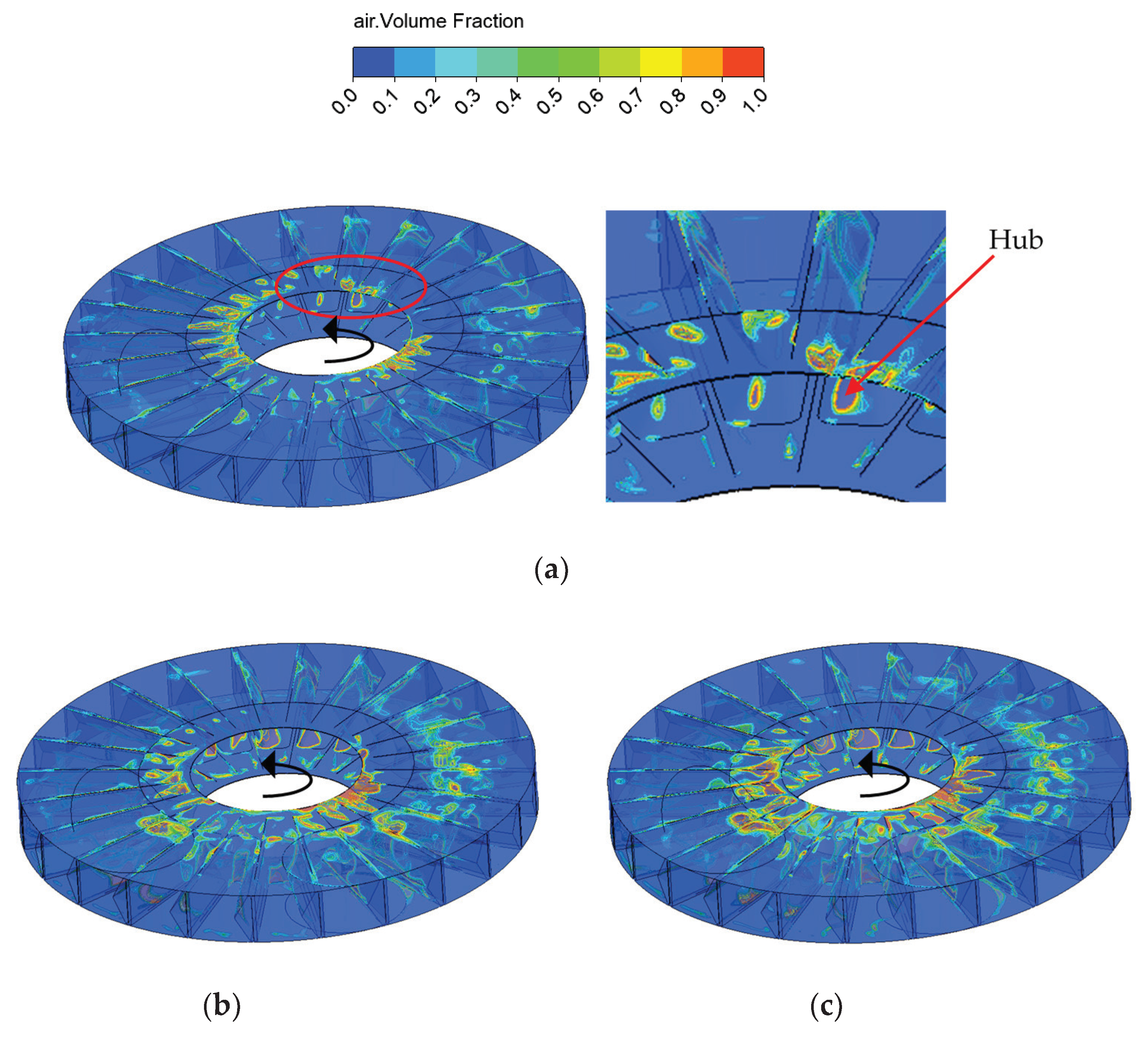
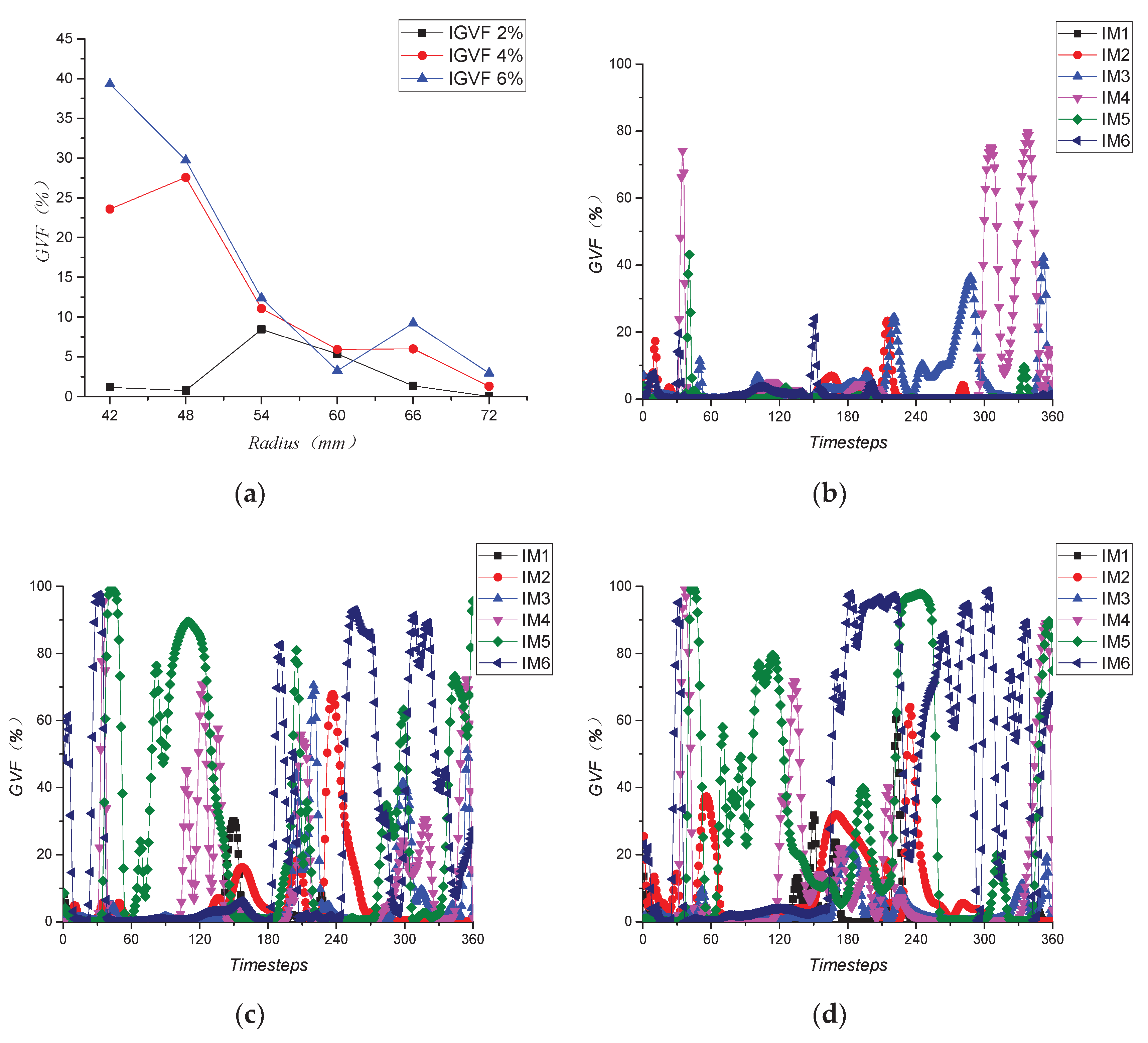
4.3.1. GVF Distribution in the Impeller

Figure 16 depicts the gas volume fraction contour on the impeller faces. The pressure and suction sides are particularly characterized with bubble formation which tends to concentrate in the middle section of the side channel. With increasing IGVF, the narrow areas where bubbles are concentrated on the suction side, and at the junction between the impeller hub and the blades, expand and spread to most of the surface. Furthermore, it can be seen clearly that the gas phase is concentrated in the axial gap in the impeller hub. On the surface in contact with the side channel, there is similar bubble distribution and the GVF is close to 100% at the inner radius close to the inlet and the outlet. In addition, with increasing the IGVF, the surface in contact with the inlet pipe is also characterized with some dispersal and small regions with high GVF. However, there exists an area that shows counter trends, as highlighted in red. When the IGVF is 2%, this region is occupied with high GVF; after increasing IGVF to 4%, the whole high GVF region disappears.

In order to further analyze the spatial distribution of the gas phase inside the flow channel of the impeller, Figure 17 shows the gas distribution in the impeller under IGVF 2%, 4%, and 6%. Compared with the pressure surface, the gas phase is obviously inclined to the suction surface. From the inlet to the outlet, under low IGVF of 2%, the initial aggregation is lumpy near the hub, when the impeller rotates 150°. The region where the bubbles congregate becomes a narrow and long strip. Moreover, the tip of the suction surface is more likely to accumulate the bubbles. When increasing IGVF to 4%, the narrow strip expands to cover the blade, but mostly they are concentrated in the upper part of the impeller close to the side channel. Under 6% IGVF, there is still no obvious gas concentrated at the outer radius of the impeller. This phenomenon demonstrates that bubbles are more easily formed at the inner radius than at the outer radius. Furthermore, there always exists a significant quantity of gas in the axial clearance under different IGVF because of very small gaps causing the bubbles difficult to flow out.

4.3.2. GVF Variations

Figure 18 shows the variation of air volume fraction at different radii under different IGVF. The average values of GVF were taken from the last complete cycle, which adds up to 360 timesteps of each monitoring point. According to Figure 17a, there is a great difference in the general trend of GVF variation under IGVF 2% compared to 4% and 6%.

Only a small amount of bubbles, or none, exist at the outer and inner radii of the impeller under IGVF 2%. The maximum of the average GVF is at the radius 54 mm with value less than 10%. This confirms that the gas phase mainly concentrates at the middle of the impeller passage under low GVF. However, when the IGVF increases to 2%, the tendency completely differs. The GVF suddenly rises significantly at the radius from 42 mm to 48 mm. At 48 mm the GVF increases from almost 0.75% to 27.6% with a difference of almost 27%. There is a marked decline of about 15% from radius 48 mm to 54 mm with a steady downward trend to the outer radius of the impeller. Furthermore, after exceeding the IGVF to 6%, the value of GVF at the inner radius increases further, and the highest GVF point is 40%. However, the percentage of the GVF at the outer radius from 66 mm to 72 mm depicts no obvious deviation compared to sudden rise at the inner radius. When the mixed fluid rotates in the impeller passage, the density of the gas phase is much lower than the liquid phase, so the gas phase moves towards the center of the impeller. The centrifugal force affects the gas movement, causing more bubbles to concentrate at the inner radius than the outer radius.

Like the average GVF value, the variation curves of different timesteps at each monitoring point under different IGVF are quite irregular, as shown in Figure 18b–d. All the monitoring points set in the inlet region are defined as the initial position, thus time steps 0° and 300° refer to the inlet and outlet regions, respectively.

Under IGVF 2%, the gas phase cannot fully develop in the impeller passage. Bubbles are mainly concentrated on the suction side of the blade as shown in Figure 18, therefore the GVF at these monitoring points is low and uneven. However, it can be observed that the fluctuation peaks always occur when the impeller rotates from 30° to 60° and 270° to 330°. Regions 30°–60° correspond to the region where the fluid just flows out from the inlet pipe, while regions 270°–330° correspond to the region where the fluid just flows into the outlet region and also flows in the interrupter; these areas all have the sudden geometry change. After ventilating another 2% IGVF, common flow patterns are observed as discussed earlier. The GVF at the outer radius is always the lowest and relatively high at the inner radius. Obviously, IM6, IM5, and IM4 from the inner to middle radii concentrate gas phase near the inlet region with values up to 100%. In addition, although the average GVF at IM6 and IM5 are high, the maximum regions appear at different time steps: IM6 is from 240° to 330°, while IM5 is from 60° to 150°.

As a final point, IGVF 4% displays the same general trend as IGVF 6%, but the GVF at IM6 maintains high values. An average deviation of 15% is recorded from IGVF 4% to 6%. On the whole, an increase of the IGVF will lead to the rise of the GVF in the impeller, especially at the inner radius. Again, the variation of the GVF easily reaches the maximum when the impeller rotates to where the side channel geometry suddenly changes.

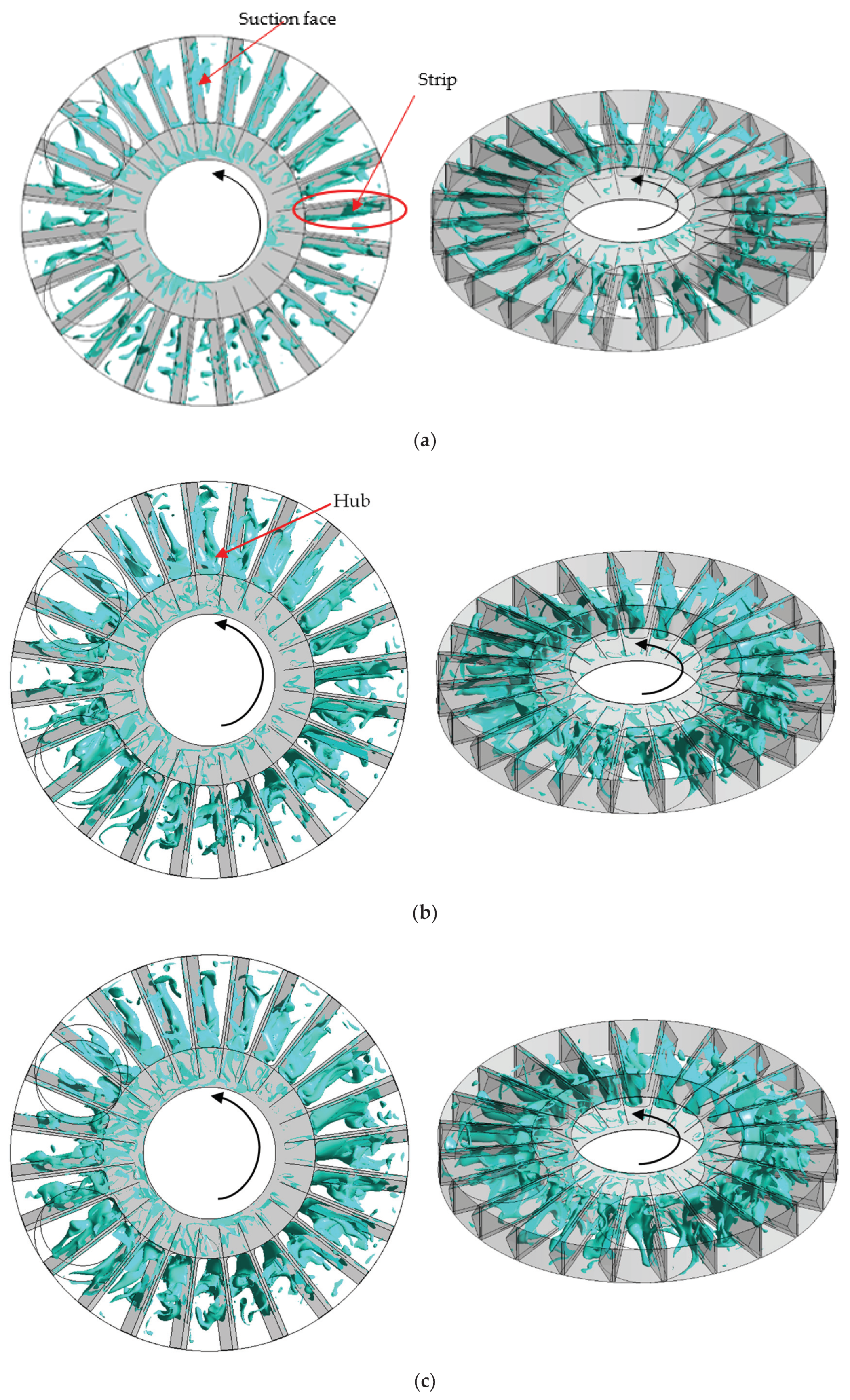
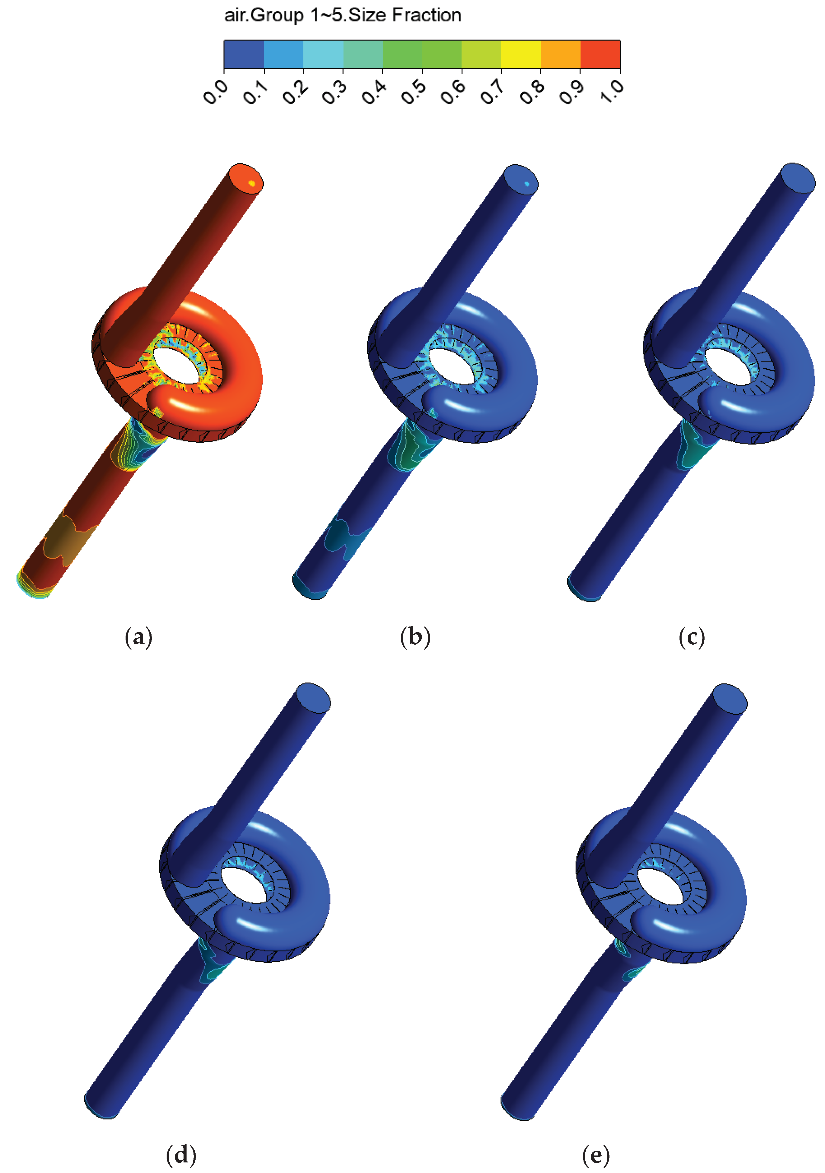
4.3.3. Bubble Diameter Distribution in the Entire Flow Domain

To show the distribution of different diameter groups in the entire flow domain, Figure 19 shows that the gas size fraction contour of bubble diameters ranges from 0.1 to 3 mm and is equally divided into five groups under IGVF 6%. The diameter distribution of Group 1 significantly differs from the other four groups. The diameters of bubbles in this group almost fill the whole fluid domain, due to the special operation mode of side channel pumps. There is a stronger shear turbulence flow in different directions with high velocity of large diameters, thus causing them to break. This explains why a low fraction is composed of high diameter bubbles. However, at the inner radius of the axial gap, this region is occupied by different groups of bubbles and is also where the air volume fraction is highest. In addition, there are two axial gaps: one is close to the inlet pipe, while the other is close to the side channel. Apparently, a high diameter area in the axial gap close to the inlet pipe occupies more proportion than in the clearance close to the side channel. In particular, bubbles with the largest diameter in Group 5 still exist, with 3 mm bubbles in the axial gap close to the inlet pipe. Furthermore, in the middle section of the axial gap close to the side channel, the diameter of bubbles is always smaller than other regions in the axial gap, which is consistent with Figure 16 above.

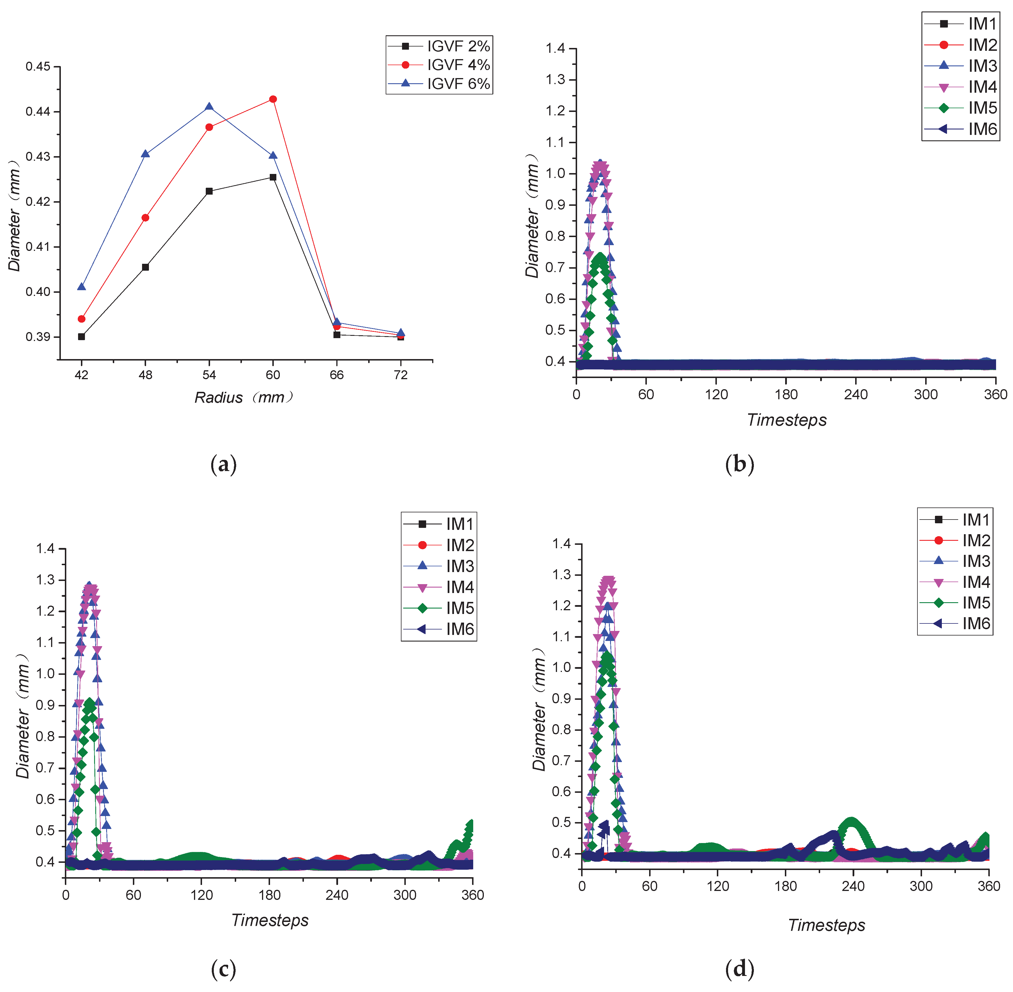
4.3.4. Bubble Diameter Variations

Figure 20 shows the particle mean diameter of bubbles of each monitoring point. In general, the particle mean diameter of bubbles in the impeller is similar. The difference between the maximum and minimum values is only 0.06 mm. Compared to the significant change of GVF curves when IGVF increases from 2% to 4%, there is no remarkable difference in the transformation rules of air particle mean diameter. The mean diameter first increases to a peak and then sharply declines to a flat pattern, and the highest points usually occur at the radii 54 mm and 60 mm in the middle of the impeller blades. A similar tendency is observed under IGVF = 6%.

For the purposes of exploring the evolution of the particle mean diameter of bubbles, the mean diameter was studied under different IGVF values for a complete revolution, as rendered in Figure 20b–d. Significant differences between GVF and diameter are revealed. The regions of large diameters over 0.8 mm, almost double the average, exist only from 0° to 30°, which is close to the inlet region, especially at IM3 and IM4. After rotating 30°, the diameter variation becomes stable with diameter near 0.4 mm, except the range 330°–360° at IM5 under IGVF 4%. According to 210°–270° at IM5 under IGVF = 6%, the deviation is less than 0.1 mm.

Overall, due to the strong shear turbulent flows of different directions in the impeller, especially on the boundaries, the bubble diameters are small and bubbles only exist in the inlet region.

4.3.5. Bubble Diameter Variation at Different Heights

To clearly analyze the air mean diameter in the impeller, three planes in the xy direction were created and set in different positions. The specific location was z₁ = 0 mm, z₂ = 7.5 mm, z₃ = 15 mm, corresponding to plane 1, plane 2, and plane 3, respectively. Figure 21 shows the three planes set in the impeller.

Figure 22 shows the air particle mean diameter distribution contour in the impeller at planes 1, 2, and 3 under different IGVF. The air particle mean diameter at the same level from an overall perspective, except for the part near the inlet pipe, corresponds to chart 1 for almost all bubbles of diameter 0.3–0.4 mm. This means that the bubble diameters are in a stable range. Due to the geometry change at the region where the fluid is about to enter the impeller, plane 1, which is close to the inlet pipe, shows a large area with high diameter bubbles (>1 mm). This nearly covers the whole face between the first three blades (colored in red). However, it can be observed that the high diameter area shrinks suddenly in plane 2 compared with plane 1. This confirms that large bubbles are broken during the movement in the impeller after flowing out from the inlet pipe. In addition, the inflow regions show a big difference in high diameter bubbles in plane 3 compared to planes 1 and 2. Here is located a very small high diameter area which nearly disappears. In addition to the inlet regions, the inner radius close to the outlet region also experiences little change: the particle mean diameter increases by approximately 0.1–0.2 mm due to a sudden change of axial velocity to vertical velocity. Hence, on account of strong shear turbulence flow in the impeller, it is hard to form large bubbles because they easily break. However, the large number of strong vortexes in different directions also creates numerous bubbles causing a high gas volume fraction.

In summary, from the charts and figures it can be established that IGVF has relatively little effect on the diameter of bubbles but a significant effect on the GVF in the impeller and side channel. The main simulation characteristics of gas phase change in gas–liquid two-phase flow in the pump relates to the GVF in the pump. However, due to the special structure and flow patterns in the side channel pump, there is a significant difference with vane pumps in general. The MUSIG model shows its heterogeneity in side channel pump gas–liquid two-phase simulation.

5. Conclusions

In this study, a new two-phase MUSIG model was applied in the side channel pump under gas–liquid two-phase flow. Due to the special structure and flow patterns in side channel pumps, there is a significant difference with other vane pumps. Therefore, the MUSIG model shows its heterogeneity in side channel pump gas–liquid two-phase simulations. The unsteady flow patterns inside the side channel pump were investigated systematically, and some conclusions can be obtained as follows:

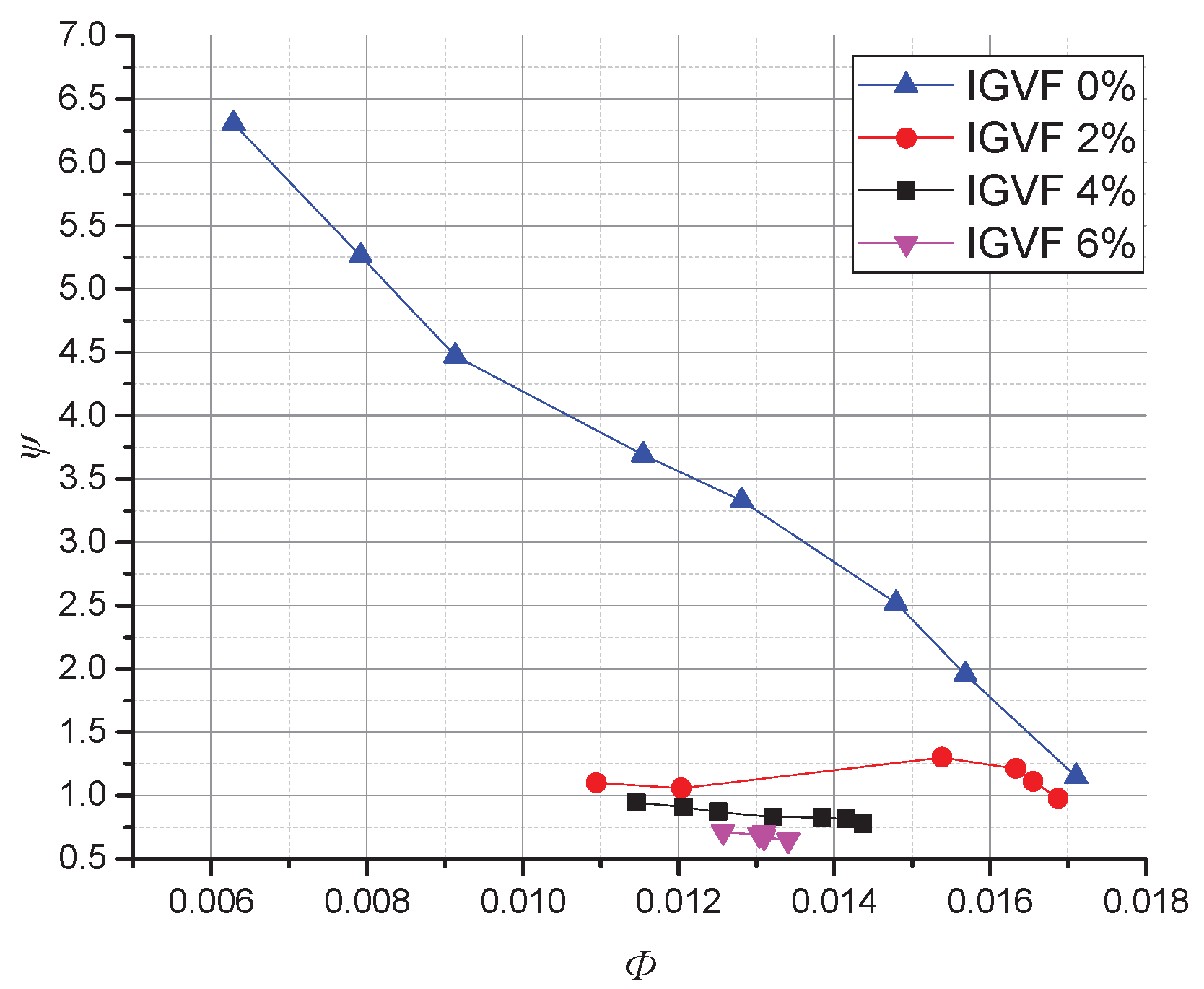
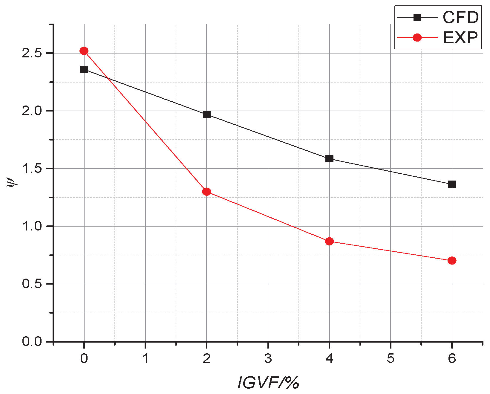
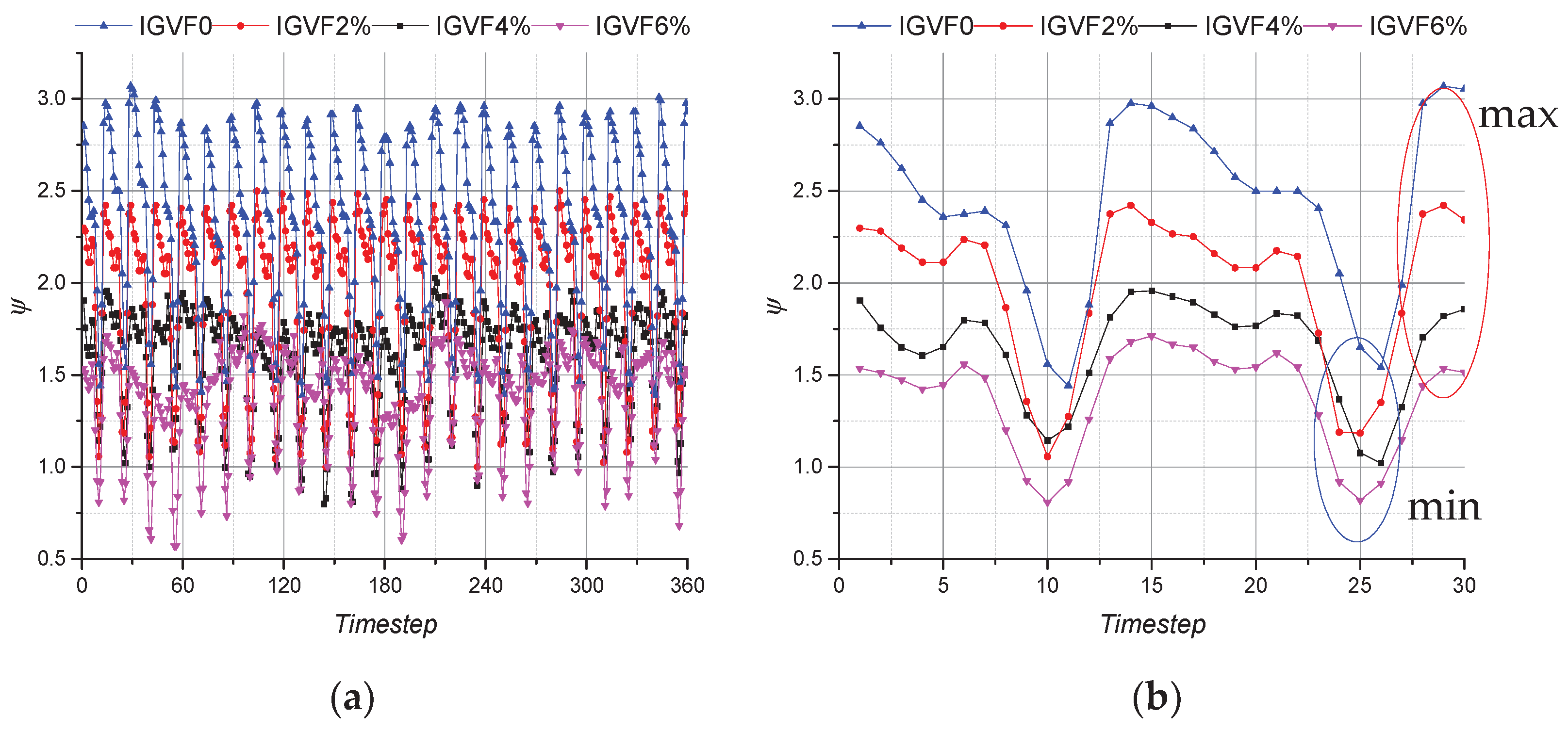
• With increasing IGVF, the pump performance tends to have an obvious degradation and the operation range of the hydraulic head becomes shortened. Thus, the side channel pump is significantly sensitive to the inlet gas quantity.
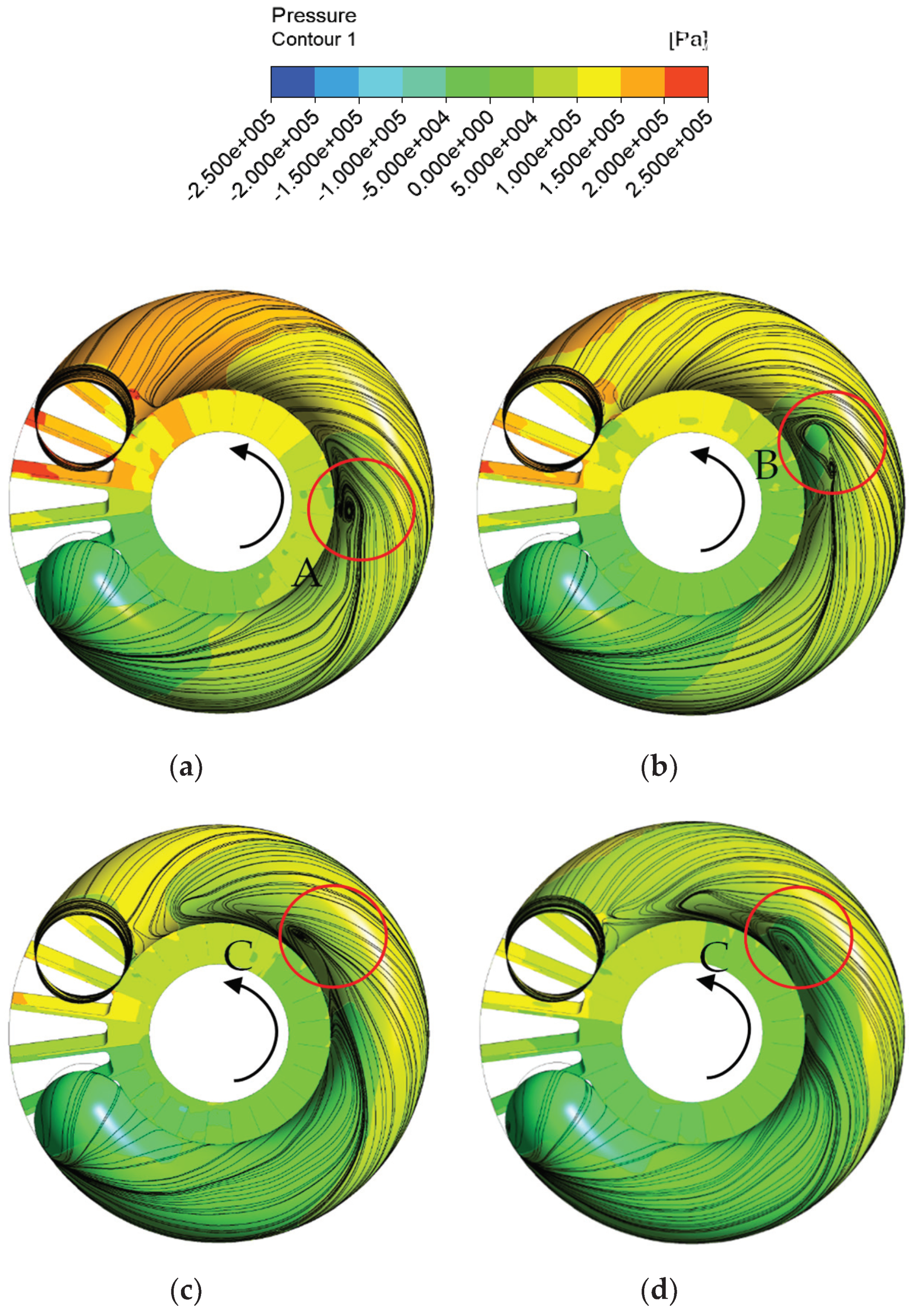
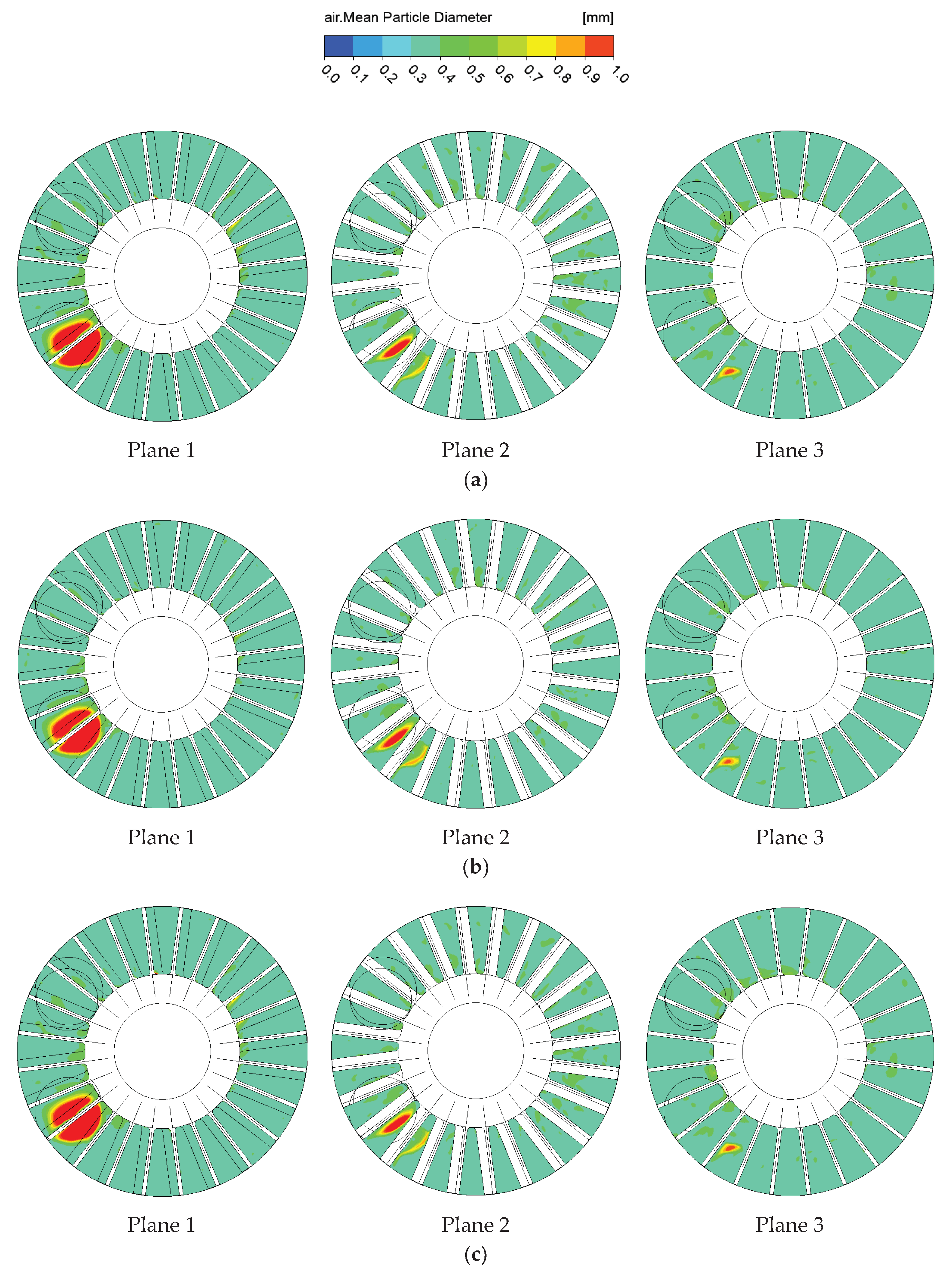
• The suction side of the blade is more likely to concentrate bubbles, especially near the inner radius of the blades where the GVF is always double that of other regions. However, at the outer radius of the impeller, there is very little or no gas.
• In general, the diameter of bubbles in the impeller and side channel are similar and small for most regions due to the strong shear turbulence flow, which eliminates large bubbles, except for the inner radius of axial gap. In the impeller, the diameter of bubbles in the middle of the blades is also relatively higher than for other parts.
• In addition, once mixture fluid goes into the impeller from the inlet pipe, the large bubbles break immediately. No gas hold up will occur in the impeller passage caused by large bubbles. Thus, this is why all side channel pumps have the capacity to deliver gas–liquid two-phase flow.
• Finally, this study reveals that the GVF and large diameter are mainly concentrated at the inner radius and gaps close to the inlet region. Therefore, to process higher amounts of gas during oil exploration and transportation of volatile chemicals, an additional gas-out hole is recommended in this region.

References

1. Kosmowski, I. Behavior of centrifugal pump when conveying gas entrained liquids. In Proceedings of the 7th Technical conference of BPMA, Cranfield, UK, July 1981; pp. 283–291. [Google Scholar]
2. Appiah, D.; Zhang, F.; Yuan, S.Q.; Osman, M.K. Effects of the Geometrical Conditions on the Performance of a Side Channel Pump: A review. Int. J. Energy Res. 2018, 42, 416–428. [Google Scholar] [CrossRef]
3. Siemen, O.; Hinsch, J. A Circulation Pump Which Acts Partially with Sealing Circling Auxiliary Liquid. Germany Patent 413435, 3 March 1920. [Google Scholar]
4. Ritter, C. About Self-Priming Centrifugal Pumps and Experiments on a New Same Kind of Pump; Phd TU Dresden: Dresden, Germany, 1930. [Google Scholar]
5. Rchmiedchen, W. Investigations on Centrifugal Pumps with Lateral Ring Channel; Phd TU Dresden: Dresden, Germany, 1932. [Google Scholar]
6. Surek, D. The influence of the geometry of the blade on the gradient of characteristic lines of side channel machines. Res. Eng. 1998, 64, 17382. [Google Scholar]
7. Fleder, A.; Böhle, M. A Study of the Internal Flow Structure in a Side Channel Pump. In Proceedings of the ISROMAC-14, Honolulu, HI, USA, 27 February–2 March 2012. [Google Scholar]
8. Fleder, A.; Böhle, M. A Systematical Study of the Influence of Blade Length, Blade Width and Side Channel Height on the Performance of a Side Channel Pump. ASME J. Fluid Eng. 2015, 137, 121102. [Google Scholar] [CrossRef]
9. Zhang, F.; Appiah, D.; Yuan, S.Q. Energy loss evaluation in a side channel pump under different wrapping angles using entropy production method. Int. Commun. Heat Mass Transfer 2020, 113, 104526. [Google Scholar] [CrossRef]
10. Zhang, F.; Böhle, M.; Yuan, S.Q. Experimental investigation on the performance of a side channel pump under gas–liquid two-phase flow operating condition. Proc. Inst. Mech. Eng. Part A J. Power Energy 2017, 231, 645–653. [Google Scholar] [CrossRef]
11. Fleder, S.; Hassert, F.; Böhle, M. Influence of Gas-Liquid Multiphase-Flow on Acoustic Behavior and Performance of Side Channel Pumps. In Proceedings of the ASME 2017 Fluids Engineering Division Summer Meeting, Waikoloa, HI, USA, 30 July–3 August 2017. [Google Scholar]
12. Minemura, K.; Murakami, M. Effects of entrained air on the performance of a centrifugal pump (first report, performance and flow conditions). Bull. JSME 1974, 17, 1047–1055. [Google Scholar]
13. Minemura, K.; Murakami, M. Effects of entrained air on the performance of a centrifugal pump (second report, effects of number of blades). Bull. JSME 1974, 17, 1286–1295. [Google Scholar]
14. Verde, W.; Biazussi, J.; Sassim, N. Experimental study of gas-liquid two-phase flow patterns within centrifugal pumps impellers. Exp. Therm. Fluid Sci. 2017, 85, 37–51. [Google Scholar] [CrossRef]
15. Furuya, O. An analytical model for prediction of two-phase(noncondensable) flow pump performance. J. Fluids Eng. (Trans. ASME) 1985, 107, 139–147. [Google Scholar] [CrossRef]
16. Minemura, K.; Tomomi, U. Prediction of air-water two-phase flow performance of a centrifugal pump based on one-dimension two-fluid model. J. Fluids Eng. (Trans. ASME) 1998, 120, 327–334. [Google Scholar] [CrossRef]
17. Poullikkas, A. Compressibility and condensation effects when pumping gas-liquid mixtures. Fluids Dyn. Res. 1999, 25, 55–62. [Google Scholar] [CrossRef]
18. Si, H.; Su, X.; Jing, G. Unsteady numerical simulation for gas–liquid two-phase flow in self-priming process of centrifugal pump. Sci. Technol. Rev. 2014, 85, 694–700. [Google Scholar]
19. Wu, Y.L. Three-dimension calculation of oil-bubble flows through a centrifugal Pump impeller. In Proceedings of the Third Internal Conference on Pump and Fan; Tsinghua University Press: Beijing, China, 1998; pp. 526–532. [Google Scholar]
20. Barrios, L.; Prado, M.G. Modeling two phase flow inside an electrical submersible pump stage. J. Energy Resour. Technol. 2009, 133, 227–231. [Google Scholar]
21. Xiaojun, L.; Bo, C.; Xianwu, L.; Zuchao, Z. Effects of flow pattern on hydraulic performance and energy conversion characterisation in a centrifugal pump. Renew. Energy 2020, 151, 475–487. [Google Scholar]
22. Lo, S. Application of the MUSIG model to bubbly flows. AEA Technology AEAT-1096 1996, 230, 8216–8246. [Google Scholar]
23. Lucas, D.; Krepper, E.; Prasser, H.M. Evolution of flow patterns, gas fraction profiles and bubble size distributions in gas-liquid flows in vertical tubes. Trans. Inst. Fluid-Flow Machinery 2003, 112, 37–46. [Google Scholar]
24. Krepper, E.; Lucas, D.; Prasser, H. On the modelling of bubbly flow in vertical pipes. Nucl. Eng. Design 2005, 235, 597–611. [Google Scholar] [CrossRef]
25. Krepper, E.; Lucas, D.; Frank, T. The inhomogeneous MUSIG model for the simulation of polydispersed flows. Nucl. Eng. Des. 2008, 238, 1690–1702. [Google Scholar] [CrossRef]
26. Liao, Y.; Lucas, D. A literature review of theoretical models for drop and bubble breakup in turbulent dispersions. Chem. Eng. Sci. 2009, 64, 3389–3406. [Google Scholar] [CrossRef]
27. Frank, T.; Zwart, P.; Krepper, E. Validation of CFD models for mono- and polydisperse air–water two-phase flows in pipes. Nucl. Eng. Des. 2008, 238, 647–659. [Google Scholar] [CrossRef]
28. Liao, Y.; Lucas, D. A literature review on mechanisms and models for the coalescence process of fluid particles. Chem. Eng. Sci. 2010, 65, 2851–2864. [Google Scholar] [CrossRef]
29. Liao, Y.; Lucas, D.; Krepper, E. Development of a generalized coalescence and breakup closure for the inhomogeneous MUSIG model. Nucl. Eng. Des. 2011, 241, 1024–1033. [Google Scholar] [CrossRef]
30. Liao, Y.; Rzehak, R.; Lucas, D. Baseline closure model for dispersed bubbly flow: Bubble coalescence and breakup. Chem. Eng. Sci. 2015, 122, 336–349. [Google Scholar] [CrossRef]
31. Bhole, M.; Joshi, J.; Ramkrishna, D. CFD simulation of bubble columns incorporating population balance modeling. Chem. Eng. Sci. 2008, 63, 2267–2282. [Google Scholar] [CrossRef]
32. Yeoh, G.; Tu, J. Population balance modelling for bubbly flows with heat and mass transfer. Chem. Eng. Sci. 2004, 59, 3125–3139. [Google Scholar] [CrossRef]
33. Sherman, C.; Yeoh, G.; Tu, J. Population balance modeling of bubbly flows considering the hydrodynamics and thermomechanical processes. Aiche J. 2008, 54, 1689–1710. [Google Scholar]
34. Zhang, F.; Appiah, D.; Zhang, J.F. Transient flow characterization in energy conversion of a side channel pump under different blade suction angles. Energy 2018, 161, 635–648. [Google Scholar] [CrossRef]
35. Celik, I.; Ghia, U. Procedure for Estimation and Reporting of Uncertainty Due to Discretization in CFD Applications. J. Fluids Eng. 2008, 130, 078001. [Google Scholar]
36. Pei, J.; Fan, Z.; Appiah, D. Performance prediction based on effects of wrapping angle of a side channel pump. Energies 2019, 12, 139. [Google Scholar] [CrossRef] [Green Version]
37. Wang, Y.F.; Zhang, F.; Yuan, S.Q. Effect of Unrans and Hybrid Rans-Les Turbulence Models on Unsteady Turbulent Flows Inside a Side Channel Pump. ASME J. Fluids Eng. 2020, 142, 061503. [Google Scholar] [CrossRef]
38. Menter, F. Two equation k-w turbulence models for aerodynamic flows. In Proceedings of the 23rd Fluid Dynamics, Plasma dynamics, and Lasers Conference, Orlando, FL, USA, 6–9 July 1993; p. 2906. [Google Scholar]
39. Menter, F. Two-equation eddy-viscosity turbulence models for engineering applications. AIAA J 1994, 32, 1598–1605. [Google Scholar] [CrossRef] [Green Version]
40. ANSYS, Inc. ANSYS Academic Research, Release 15.0, Help System, ANSYS CFX-Solver Theory Guide; 15317; ANSYS, Inc.: Canonsburg, PA, USA, 2013. [Google Scholar]
41. Luo, X.W.; Ji, B. A review of cavitation in hydraulic machinery. J. Hydrodyn. 2016, 28, 335–358. [Google Scholar] [CrossRef]
42. Bachert, B.; Brunn, B.; Stoffel, B. Experimental Investigations Concerning Influences on Cavitation Inception at an Axial Test Pump. In Proceedings of the ASME-JSME Joint Fluids Summer Engineering Conference, Honolulu, HI, USA, 6–10 July 2003. [Google Scholar]
43. Pei, J.; Osman, M.K.; Wang, W. Unsteady flow characteristics and cavitation prediction in the double-suction centrifugal pump using a novel approach. Proc. Institut. Mech. Eng. Part A J. Power Energy 2019. [Google Scholar] [CrossRef]
44. Zhang, F.; Chen, K.; Appiah, D. Numerical Delineation of 3D Unsteady Flow Fields in Side Channel Pumps for Engineering Processes. Energies 2019, 12, 1287. [Google Scholar] [CrossRef] [Green Version]
Figure 1. Fluid pathways in side channel pump.
Mathematics 08 00624 g001
Figure 2. 3D model of a side channel pump.
Mathematics 08 00624 g002
Figure 3. Computational fluid domains of the side channel pump ((1) inlet; (2) impeller and gaps; (3) outlet and side channel).
Mathematics 08 00624 g003
Figure 4. Partial mesh view of the flow domain: (a) inlet pipe, (b) side channel, (c) impeller and gaps.
Mathematics 08 00624 g004
Figure 5. Mesh independence.
Mathematics 08 00624 g005
Figure 6. Velocity streamlines in the middle plane of the impeller under different grid numbers. (a) 3.7 million (b) 4.0 million (c) 4.5 million (d) 4.8 million (e) 5.0 million.
Mathematics 08 00624 g006aMathematics 08 00624 g006b
Figure 7. Monitoring points.
Mathematics 08 00624 g007
Figure 8. Experimental setup.
Mathematics 08 00624 g008
Figure 9. Head comparison under different inlet gas volume fraction (IGVF).
Mathematics 08 00624 g009
Figure 10. Performance curve comparison of the test pump.
Mathematics 08 00624 g010
Figure 11. Head fluctuation curve. (a) The fluctuation in a completed revolution (b) The maximum and minimum point
Mathematics 08 00624 g011
Figure 12. Pressure and velocity streamlines in side channel wall (a) single phase, (b) IGVF 2%, (c) IGVF 4%, (d) IGVF 6%.
Mathematics 08 00624 g012
Figure 13. Plane zx.
Mathematics 08 00624 g013
Figure 14. Pressure and velocity streamlines between impeller and side channel: (a) single phase, (b) IGVF 2%, (c) IGVF 4%, (d) IGVF 6%.
Mathematics 08 00624 g014
Figure 15. Pressure and velocity streamlines between impeller and side channel. (a) single phase, (b) IGVF 2% air, (c) IGVF 2% liquid, (d) IGVF 4% air, (e) IGVF 4% liquid, (f) IGVF 6% air, (g) IGVF 6% liquid.
Mathematics 08 00624 g015aMathematics 08 00624 g015b
Figure 16. Gas volume fraction distribution under different IGVF. (a) IGVF 2%, (b) IGVF 4%, (c) IGVF 6%.
Mathematics 08 00624 g016
Figure 17. Gas distribution counter in the impeller under different IGVF and GVF equal to 30%. (a) IGVF 2% under GVF 30%, (b) IGVF 4% under GVF 30%, (c) IGVF 6% under GVF 30%.
Mathematics 08 00624 g017
Figure 18. GVF change under different IGVF, (a) average, (b) IGVF 2%, (c) IGVF 4%, (d) IGVF 6%.
Mathematics 08 00624 g018
Figure 19. Gas size fraction of different bubble diameters under IGVF 6%. (a) group1, (b) group2, (c) group3, (d) group4, (e) group5.
Mathematics 08 00624 g019
Figure 20. Diameter change under different IGVF at same angle and radius. (a) average, (b) IGVF 2%, (c) IGVF 4%, (d) IGVF 6%.
Mathematics 08 00624 g020
Figure 21. Three axial planes on the impeller.
Mathematics 08 00624 g021
Figure 22. Diameter distribution under different IGVF. (a) IGVF 2%, (b) IGVF 4%, (c) IGVF 6%.
Mathematics 08 00624 g022