Abstract
“Discretization” usually denotes the operation of mapping continuous functions to infinite or finite sequences of discrete values. It may also mean to map the operation itself from one that operates on functions to one that operates on infinite or finite sequences. Advantageously, these two meanings coincide within the theory of generalized functions. Discretization moreover reduces to a simple multiplication. It is known, however, that multiplications may fail. In our previous studies, we determined conditions such that multiplications hold in the tempered distributions sense and, hence, corresponding discretizations exist. In this study, we determine, vice versa, conditions such that discretizations can be reversed, i.e., functions can be fully restored from their samples. The classical Whittaker-Kotel’nikov-Shannon (WKS) sampling theorem is just one particular case in one of four interwoven symbolic calculation rules deduced below.
Keywords:
regularization; localization; truncation; cutoff; finitization; entirization; cyclic dualities; multiplication of distributions; square of the Dirac delta; Whittaker-Kotel’nikov-Shannon MSC:
42B05; 42B08; 42B10; 46F05; 46F10
1. Introduction
The theory of generalized functions [1,2,3,4,5,6,7,8,9,10,11,12,13,14,15,16,17,18,19,20,21,22,23,24,25,26,27,28,29,30,31,32,33,34,35,36,37,38,39,40,41] is a standard setting today, not only in mathematics, in particular, Fourier [42,43,44,45,46,47,48,49,50,51,52,53] and wavelet analysis [54,55,56,57], but also in physics [58,59,60,61,62,63,64,65,66,67,68,69,70,71,72,73,74] and in electrical engineering [75,76,77,78,79,80,81]. It has already proved to be helpful for finding a simple validity statement for Poisson’s Summation Formula [82], an explanation for Heisenberg’s uncertainty principle [83], the insight that four Fourier transform definitions are actually all the same Fourier transform [84] and, eventually, to understand the multiplication difficulties (Figure 1, Section 2, Lemma 1) among generalized functions which led us to a better understanding of the “square of the Dirac delta”, in what sense it exists and in what sense it does not exist [85].
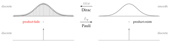
Figure 1.
Multiplication products, discrete–discrete fails, discrete–smooth products exist.
Within generalized functions theory, all functions and generalized functions are infinitely differentiable. It implies simple answers to questions which concerned researchers for decades, see e.g., [26], Charts 1–2, pp. 222–223. The theory of generalized functions, distribution theory, is for example a valuable tool for solving ordinary and partial differential equations [11,28,29,30,86,87,88,89], also fractional differential equations [81,90,91,92]. Hence, it is a key instrument to describe natural laws. Above all, it extends the idea of Fourier transformation because not only integrable but also constant, polynomially growing, even exponentially growing functions can now be Fourier transformed. Finally, it also allows us to treat Dirac delta functions [93] and Dirac combs [94] just as if they were ordinary functions but with adequate mathematical rigor.
Here, we continue a series of studies [82,83,84,85] towards a sampling theorem on tempered distributions. The present study is, more precisely, the second half of [85] which is a foundation for this one. Our primary goal is the embedding of the Whittaker-Kotel’nikov-Shannon sampling theorem [95,96,97,98,99,100,101,102,103,104,105] in generalized functions theory, more precisely, its embedding within the space of tempered distributions. Tempered distributions, in turn, lie in the intersection of distributions and ultradistributions, see Figure 1 in [85], and distributions and ultradistributions are particular hyperfunctions [106,107,108,109]. Hyperfunctions arise as a difference of pairs of holomorphic functions [26,40] and “generalized functions” are nothing else than “Randwerte”, boundary values, of these pairwise arising holomorphic functions [3,4,8]. We proceed as follows. Section 2 describes the outer framework and the motivation for these studies, Section 3 introduces to used notations and Section 4 reviews the results we have so far. Section 5 presents new results, it introduces to four kinds of “truncation”, sharp and smooth truncation in both time and frequency domain, and their respective symbolic calculation rules. They are needed in Section 6 which is our main result. It consists of two halves (Theorems 1 and 2) of a theorem on “Cyclic Dualities” (Theorem 3), a statement on the Fourier duality between two commonly known identities (periodicity-finiteness and discreteness-entireness). Section 7 is an important consequence. It allows us to discretize already discrete functions and to periodize already periodic functions. Section 8, finally, concludes this study.
2. Motivation
2.1. Scale of Observation
Once, Mandelbrot asked the question “How long is the coast of Britain?” and the answer is infinite, unless the “scale” , the smallest measuring unit, is specified [110]. Equivalently, the multiplication product between two Dirac delta functions remains undetermined (Figure 1), unless their relative “position uncertainty” is known [85]. In any measurement, some uncertainty is present (Figure 2, left) because measuring devices with infinite bandwidth do not exist. A key finding in renormalization theory [111] is the fact that measurement results depend on the “scale” of observation [112]. The “scale” is moreover well-known in optical and radar imaging, in terms of the chosen “frequency band” [113], “resolution” [114] and “pixel size” [115,116], denoted T (Figure 2).
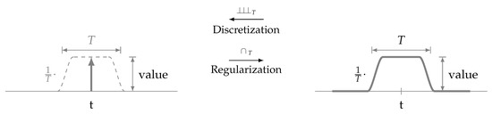
Figure 2.
Equivalent pixel representations, Dirac’s delta (left) and Lighthill’s unitary function (right).
The “scale” is also known in wavelet analysis [54,55,57,117]. Each “pixel”, often denoted using a Dirac delta [50,57,77,79,118,119,120,121,122,123], does not only have a (1) position and a (2) value but also a (3) width, given by as a consequence of the finite bandwidth B of a used measuring device (Appendix C). One may recall, B may be large but cannot be infinite. Hence, for every sample (Dirac delta), there is a corresponding scale greater than zero (Figure 2, left). Vice versa, choosing in , “discretization” ceases to exist (see Definition 1). The pixel size is, so to say, a hidden property of any Dirac delta. It is its smoothness component, the “scale” at which we are able to “see”, a tiny surface interacting with matter. In radar remote sensing, for example, we are able to “see” clouds at short (<3 cm) wavelengths and we are able to “see” (the ground) through clouds at longer (>3 cm) wavelengths [113,124]. So, the “things” we “see” depend on the scale of observation.
2.2. Discretization versus Regularization
In the history of quantum mechanics, two opposite positions can be found, Dirac, on one side, with his functions as the representatives of discreteness, i.e., infinitely precise (position or momentum) measurements and Pauli [111,125,126] on the other who regularized functions in order to obtain smoothness, i.e., to get rid of improper functions and the infinities they introduce. The intention of Pauli was to introduce mathematical rigor into “renormalization” theory [111], initiated by Heisenberg and developed by Schwinger, Feynman and others [36]. His idea was to smear out “sharp” results (Figure 1) and in this way to regain regular (smooth) functions, i.e., functions which possess a “norm” in contrast to improper functions. However, both strategies, Dirac’s and Pauli’s, are correct from a strict mathematical point of view (distribution theory). They are, in fact, “dual” to one another, i.e., one strategy cannot exist without the other. It is expressed in the reciprocal relationships (Theorem 3)
between discretization and two kinds of regularization, and , at a respective scale T (see an example in Figure A6), ∘ is the concatenation of operations and id is the identity operation. The reason why can be replaced by and vice versa is Lemma 5 in [85]. Regularization [11,13,14,15,17,30,35,49] is well-established today, used for example in [47,69,91,111,125,126,127,128,129,130]. It is the inverse operation of discretization ([14], p. 132 and [15], p. 401). Localization is another most important tool, e.g., in [13,65,131,132,133,134,135,136]. It is the Fourier dual of regularization [83,136]. A particular case of localization is truncation [137,138,139,140,141] and a link between discretization, truncation and “Tikhonov regularization” is studied in [128,129]. In generalized functions theory, we replace the “Picard condition” by (see Tables 1–3, [84]). It ensures that f falls to zero with exponential decay, cf. [133]. Equivalent is the condition , see Lemma 1. It ensures that is an ordinary, infinitely differentiable function [41].
2.3. Regularization Methods
All together, there are four regularization methods and in [85] we showed that all four are exactly those which reverse “discretizations” in both time and frequency domain. They correspond to four kinds of “truncation”: sharp and smooth truncation in both time and frequency domain. Their main application is a back-and-forth “sampling theorem” on generalized functions (Table A3, Rules 25–28). However, amongst other things, it also tells us how to regularize generalized functions in both time and frequency domain (simultaneously). The latter is a core demand in renormalization theory [13]. It is known that, once the “distribution multiplication problem” is solved, then the central problem in renormalization theory is solved as well.
3. Notation
All functions and generalized functions in generalized functions theory (distribution theory) are smooth (infinitely differentiable), either in the ordinary or in the generalized functions sense. In this study, we follow the standard notation in distribution theory and continue [85] where we already introduce to the topic in much greater detail. Amongst others, we explain how to deal with generalized functions and how to extend the one-dimensional case to the n-dimensional case . See [142] for a treatment in n dimensions. An example for is given in Appendix C. In this section, we merely summarize the most important facts and notations.
3.1. Fourier Transform
We denote all spaces of ordinary and generalized functions as in the standard literature, e.g., [1,14,15,27,30]. The “unitary ordinary frequency” or “normalized” Fourier transform of integrable functions is
where is the usual inner product in and for generalized functions it is for , is the application of f to [85]. We denote them as or or simply . The space of tempered distributions includes, in particular, the Schwartz space , the subspace of functions which are well-localized in both time and frequency domain.
3.2. Sinc and Rect Functions
The function is defined to be 1 at and else and is its Fourier transform. It equals 1 within the interval as well as at and and zero else. We prefer using instead of the characteristic function of an interval which cannot take on values other than 0 or 1. This “mid-point property at jumps”, cf. [43], p. 52, is a property of the Fourier transform [9,45]. It implies, for example, Rules 19 and 20 in [84]. The function belongs to , the subspace of all ordinary smooth functions in and belongs to , the subspace of rapidly decreasing generalized functions in . Vice versa, does not belong to because it is not smooth (infinitely differentiable) and does not belong to because its decrease is too slow (polynomially instead of exponentially), cf. Remark 2 in [84]. Additionally, belongs to , the subspace of compactly supported “time-limited” tempered distributions in and belongs to , the subspace of Paley-Wiener “band-limited” ordinary functions in .
3.3. Finite, Entire, Local and Regular Functions
For reasons of brevity, we call functions “finite”, “entire”, “local” and “regular” if they belong to the spaces , , and , respectively [85]. The Paley-Wiener-Schwartz-Ehrenpreis theorem [143] states that, briefly, and . It is also known in terms of the Paley-Wiener-Schwartz [46,100] or the Paley-Wiener theorem [46,133,144]. We call this the Fourier duality between time and band-limited functions. It extents to and (Lemma 1) which is the Fourier duality between time and band-localized functions. In particular, and satisfy and . Figure 1 in [85] visualizes these relations and tells us that “time or band-localization” is wider than “time or band-limitness”. A subspace of is , the space of “time-limited” Schwartz functions, and a subspace of is , the space of “band-limited” Schwartz functions [145], cf. Figure 1 in [85].
3.4. Localized Sinc, Regularized Rect, Unitary Functions and Dirac Comb
The Fourier duality between and is not directly applicable to arbitrary tempered distributions [37,49,85,127,146]. However, localized and regularized functions [13] can be applied to any tempered distribution [83]. We denote them and , respectively [85]. The function is a so-called Lighthill unitary function [7,42,58,147]. It is furthermore a “building block” of the function that is constantly 1. Hence, it forms a “smooth partition of unity” [13] and as such it plays a very central role in Fourier analysis. It serves, for example, as cutout function whenever the Fourier coefficients of a periodic tempered distribution [7,30,34] such as the “Dirac comb”
need to be determined. Here, is real-valued and extends to for ordinary functions f. We briefly write if and III if . Clearly, [35,76,148] and and , see e.g., [43,52,76,82]. The functions and are, in fact, the convolution and multiplication (cross) inverses of , see [85]. The regularization of and the localization of are both linked to “Riemann’s localization theorem” [45,134,146,149,150].
4. Preliminaries
We briefly list the most important ingredients (Lemma 1, Definition 1, Lemma 2) here. These are known facts. For details one may refer to [85].
Lemma 1
(Convolution-Multiplication Duality). Let and and , then
in the tempered distributions sense.
The conditions described in this lemma [15,17,24,27] are both necessary and sufficient for the existence of convolutions and multiplications on tempered distributions [84]. They secure, for example, the existence of the “square of the Dirac delta” in a rigorous distributional sense [85]. Using Lemma 1, we may define “discretizations” and “periodizations” as follows.
Definition 1
(Periodization and Discretization). For , and real , we define
periodization and discretization, respectively.
These operations, primarily intended for radar applications, can already be found in Woodward [151], p. 28, as and operations (cf. [84], Table 2). Woodward is known for first mentioning the function [32,43,100,152,153] and his time-frequency ambiguity function [46,51,56,154,155,156,157,158,159,160,161,162]. We now let g be the Dirac comb, it leads us to the following lemma [82,142].
Lemma 2
(Discrete Functions vs. Periodic Functions). Let be real, and , then
in the tempered distributions sense.
5. Truncation
There are, basically, four kinds of truncation. All four arise naturally as the multiplication and convolution inverses of the Dirac comb [85]. Truncation can be done sharply or smoothly, e.g., [51], p. 37, and in time or frequency domain, e.g., [100], p. 191. All four are introduced next.
5.1. Sharp Truncation
First, we distinguish between sharp truncation in time (finitization) and sharp truncation in frequency domain (entirization). The resulting functions are time-limited () or band-limited (). An explicit construction of is described in [85].
Definition 2
(Finitization). Let be real. For any , we define another tempered distribution by
where is double-sided unitary. The operation is called finitization.
Definition 3
(Entirization). Let be real. For any , we define another tempered distribution by
where is double-sided unitary. The operation is called entirization.
Finitization restricts f to an interval where may be arbitrarily small such that f is finite () and is entire (). Entirization, in turn, restricts to an interval where such that is finite and f is entire.
5.2. Smooth Truncation
A wider idea of sharp truncation (time or band-limitness) is smooth truncation (time or band-localization), e.g., [163], p. 49. Instead in and we now land in and , respectively, which include and , i.e., “time or band-limitness” is generalized in this way.
Definition 4
(Regularization). Let be real. For any , we define another tempered distribution by
where is double-sided unitary. The operation is called regularization.
Definition 5
(Localization). Let be real. For any , we define another tempered distribution by
where is double-sided unitary. The operation is called localization.
It is known that the space of “time-limited” and the space of “band-limited” functions do not overlap (except for the zero function). For this reason, a concept of “time and band-localized” functions is required. Here, the well-known Schwartz space is in its overlap (Figure 1 in [85]). Schwartz functions are, correspondingly, well-localized in both time and frequency domain. It explains their extraordinary role as (1) test functions for tempered distributions, (2) test functions in quantum mechanics [63], p. 12 and [164], pp. 317–318, (3) window functions in the Short Time Fourier Transform (STFT) [41,51,56,165,166] and (4) their validity-satisfying role in Poisson’s Summation Formula [20,84,142,165].
5.3. Four Truncation Rules
The above definitions obey the following four symbolic calculation rules. They are particular cases of a generally valid regularization-localization duality [83].
Lemma 3
(Time vs. Band-Truncation). Let be real-valued and , then
in the tempered distributions sense.
Lemma 4
(Time vs. Band-Localization). Let be real-valued and , then
in the tempered distributions sense.
Obviously, the first and the second line in both lemmas are Fourier transforms of one another. We merely prove the first lemma, the second is shown analogously.
Proof.
Let be double-sided unitary, then is again double-sided unitary [85] and belongs to . Using our operator definitions and Lemma 1,
in the tempered distributions sense. □
In engineering, Lemma 3 reduces to the trivial statement that time and band-limited functions are Fourier transforms of one another and Lemma 4 expresses the same but in a wider sense. The latter is known as the Fourier duality between windowing (localization) and smoothing (regularization). The use of mollifiers [86] and regularizers [127] has its origin here.
6. Representation Theorems
The next two theorems can be understood as representation theorems for periodic functions, discrete functions and for time and band-limited generalized functions in . The entity is known as the “time-bandwidth” product [163], cf. Woodward [151], pp. 118–119.
Theorem 1
(Global Inversion). Let be real, , be B-periodic and , then
in the tempered distributions sense.
Theorem 2
(Local Inversion). Let be real, , be B-finite and , then
in the tempered distributions sense.
Proof.
Global Inversion. Because , therefore , we have
where the second equality holds because p is B-periodic. The symbol denotes one period of p. With Lemmas 2 and 3 we now deduce that
in the tempered distributions sense. □
Although the next proof is very similar, it is presented here for comparison purposes. More precisely, (21) and (22) are needed below in Corollary 1.
Proof.
Local Inversion. Using the fact that f is B-finite, symbolically , we obtain
where the second equality holds because for and zero else. With Lemma 2 and Lemma 3 we now deduce that
in the tempered distributions sense. □
Equation (17) can also be found in Vladimirov [34], p. 114 as (1.4), in particular (1.5), for the reader’s convenience—although it is derived here differently. In the special case where p is an ordinary function, can be replaced by multiplication with the characteristic function of an interval, cf. Benedetto and Zimmermann [167], p. 508. In general, however, the cutout function is a unitary function, i.e., it is not unique [7], p. 61. Equation (18) is the Fourier transform of (17). We may think of as the “period” of p, of as the “wave” of d, of as the “cycle” of f and of as the “coefficients” of . Clearly, and as well as and are all not unique in (17)–(20). It is, hence, convenient to think of them as equivalence classes in these equations.
Equation (20) is the classical Whittaker-Kotel’nikov-Shannon (WKS) sampling theorem [95,98,101,104] in and (19) is its Fourier domain, is -multiplication and is -convolution in the limiting case. For ordinary functions, (20) and (19) coincide with (28) and (29) in [151], pp. 33–34, respectively. One may recall, sinc-convolution succeeds on Lebesgue square-integrable functions with extremely slow convergence but fails on arbitrary tempered distributions [49]. We therefore constructed as the multiplication with a “regularized” -function [13] and as the convolution with a “localized” -function in [85]. The duality between regularization and localization [83] is often used in connection with the classical sampling theorem, e.g., in [146]. Using “localized” -functions accelerates (cf. [7], p. 6, ) the convolution convergence and corresponds to the use of “regularizers” [127]. The use of regularizers, in turn, corresponds to using “oversampling” [54]. In fact, “any sampling rate higher than the Nyquist rate is sufficient” [168]. Let us remind here to the fact that functions cannot be integrated, neither in the Riemann nor in the Lebesgue sense [47,169]. However, it exists as an “improper integral” [151,170] which corresponds to using “convergence factors” [171] as, for example, in García and Moro [101]. The idea used in [101] is moreover equivalent to the use of Lighthill’s unitary functions [7,85,147], in other words, to the use of the operators and .
The condition is further studied in Appendix B. It is now just a small step to deduce the following statement. We relate finiteness to periodicity and smoothness to discreteness.
Theorem 3
(Cyclic Dualities). If is considered being cyclic and finite, simultaneously, then
in the tempered distributions sense, where . Hence, is both discrete and entire, simultaneously.
Proof.
If Theorem 1 and 2 are true and p is f and f is p then, by Fourier duality, d is and is d. □
Therefore, . The commutator [63,84] is defined as . In other words, and as well as and commute. Dualities as in (23) or (24) do indeed exist. They are, often unawarely, heavily used in practice. We give three examples.
Example 1
(Discrete Fourier Transform). Cyclic dualities are routinely used in digital signal processing. Whenever we use the Discrete Fourier Transform (DFT), we actually identify finite functions with periodic functions and periodic functions with finite functions [50]. Hence, g and are both finite and periodic. Simultaneously, and g are both entire (smooth) and discrete (Theorem 3) by Fourier duality.
Example 2
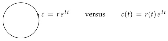
(Number-Function-Duality). Every real number is a constant function and every constant function is a real number. More generally, complex numbers are “waves” (Figure 3), cf. [172]. Thinking of 1 as a discrete periodic function, we may use the DFT, its Fourier transform is 1. Thinking of 1 as a smooth periodic function, using in , its Fourier transform is δ. One may recall, this is no contradiction [84].
Figure 3.
Complex numbers are discrete (as a number) and smooth (as a function), simultaneously.
Example 3
(Wave-Particle Duality). Cyclic dualities are moreover known in quantum physics where we either observe (discrete) positions of a particle or all its positions as an entire (smooth) wave. Its momentum (Fourier transform) is, correspondingly, smooth if its position is discrete and discrete if its position is smooth. It is known as the “wave-particle duality” and it turned out be equivalent to Heisenberg’s uncertainty principle [173].
An intimate relationship between finiteness and periodicity is also known in other branches of physics, e.g., in crystallography [94] or, more generally, whenever periodic boundary conditions arise, e.g., in [174,175]. “Dirichlet boundary conditions” emerge for example in connection with the “time-periodic” case of Maxwell’s equations in [88,89]. Here, it is intended to find real-valued, time-periodic and spatially localized solutions. Theorem 3 tells us that whenever we add periodic boundary conditions to finite or infinite intervals, i.e., as soon as we close a circle (Figure 4), it implies identifying smoothness with discreteness in its Fourier domain.
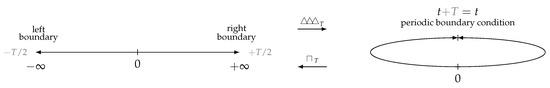
Figure 4.
The real axis before (left) and after (right) periodization, T replaces “infinity”.
Obviously, many infinities (if not all) arise by just cycling around finitely extended circles. More generally, circles can be replaced by (nearly arbitrary) closed paths in the complex plane [176,177]. Our result is obviously related to the Fundamental Theorem of Calculus ([177], Theorem 24) and Cauchy’s theorem ([177], Theorem 25). The idea that “infinity” might not exist in the real world [178] is presently hotly debated in physics [179,180]. It is moreover known in complex analysis that the “complex plane” is not a plane but a “Riemann sphere” and the “real axis” is not a line but a circle on the Riemann sphere going through its “north pole” where and coincide [3,8,9,176]. The “imaginary axis” is now another circle on the Riemann sphere, also through its north pole, but intersects the real axis orthogonally.
7. Wider Definitions
The “classical” sampling theorem (20) states that , i.e., regularization reverses discretization. Vice versa, the “forward” sampling theorem (18) states that , i.e., discretization reverses regularization. Both together yield (1). So, discrete functions can always be applied to smooth functions and smooth functions can always be applied to discrete functions. This discreteness-smoothness duality is in fact the foundation of generalized functions theory. It can be used as follows.
Definition 6
(Periodization and Discretization, revisited). For any and real , we define
periodization and discretization, respectively.
Remark 1
(Constants). This definition, in contrast to Definition 1, allows us to periodize already periodic functions and to discretize already discrete functions, e.g., and hold for any .
Remark 2
(Special Functions). One may briefly denote time-limited, band-limited, periodic or discrete functions as , , , , for some , respectively.
Convolution-Multiplication Associativity
Another beautiful detail shall be mentioned. Following Ellis [181], Novelli and Thibon [182], we call it “cross-associativity” between multiplication and convolution in . We believe this property is not known in the literature so far. It relies on Lemma 1.
Corollary 1
(Cross-Associativity). There are such that
in the tempered distributions sense.
Proof.
Corollary 1 may also be true on other tempered distributions, Schwartz functions , for example. However, most generally, multiplication or convolution products are not associative in , not in a mixture of * and · and not even among multiplication products alone, see e.g., [8]. Nevertheless, the idea that periodic functions, discrete functions as well as time and band-limited functions might exactly be those which satisfy these equations in a widest sense in is fascinating and worth being further investigated.
8. Discussion and Outlook
Woodward concludes in [151], p. 120, that “the effective ‘area of ambiguity’ in the time-frequency domain […] is equal to unity”. More precisely, he expresses this in two equations
They correspond to in this study, i.e., and , respectively. This relation between sampling rate and bandwidth B is known as the “classical sampling theorem” and it is linked herewith to Woodwards’s effective “area of ambiguity” which equals 1. The “Classical Sampling Theorem” in is summarized in Table A3, Rules 25–28. One may note, it does not matter whether T is B or B is T, both variables are fully equivalent. They are reciprocal to one another. Furthermore, is nothing else than the definition of “frequency”. It means “frequency” is “reverse time” and, trivially, “reverse time” × “time” equals unity. For a deeper understanding one may study Max Born’s theory of reciprocity [183,184].
The theorems derived in this study are in fact part of a larger symbolic calculation scheme, summarized in Appendix A. One may have noticed, four truncation methods and are introduced but only have been used intensively. According to [85], Lemma 5, it is possible to replace by and by in many cases—done e.g., in Appendix C. We will have a closer look at this phenomenon in a later study.
Author Contributions
Conceptualization, J.V.F.; Formal analysis, J.V.F.; Investigation, J.V.F.; Methodology, J.V.F.; Project administration, R.L.S.; Software, J.V.F.; Supervision, R.L.S.; Validation, R.L.S.; Visualization, J.V.F.; Writing—original draft, J.V.F.; Writing—review and editing, R.L.S. All authors have read and agreed to the published version of the manuscript.
Funding
This research received no external funding. OpenAccess publications are funded by DLR Bibliotheken.
Acknowledgments
The authors would like to thank the reviewers for their careful review and valuable suggestions and the editors of this journal for their courteous, rapid processing.
Conflicts of Interest
The authors declare no conflicts of interest.
Appendix A. Symbolic Calculation Rules
The following tables summarize the results in this study, they complement previously found rules, cf. Tables 1–3 in [84]. All rules below are given pairwise, i.e., two consecutive lines are Fourier transforms of one another where . Hence, and , respectively.
The unitary function , see Rules 01, 03 and 07, is a generalization of the characteristic function (cf. [57], p. 47, [53], p. 3, [105], p. 570) on the interval and is its Fourier transform. At the same scale, and are two different pixel representations (Figure A6, left and right). Table A1 and Table A2 are both generalized in Table A3. The properties “finite” and “entire” are inherited from unitary functions and “discrete” and “periodic” are inherited from Dirac combs.

Table A1.
Unitary Functions—Synthesis & Analysis.
Table A1.
Unitary Functions—Synthesis & Analysis.
| No | Rule | Remark | Operation | Result |
|---|---|---|---|---|
| 01 | Synthesis of = Analysis of 1 | Time-Truncation of 1 | finite | |
| 02 | Synthesis of = Analysis of | Band-Truncation of | entire | |
| 03 | Analysis of = Synthesis of 1 | Periodization of | periodic | |
| 04 | Analysis of = Synthesis of | Discretization of | discrete | |
| 05 | Rule 01 + Rule 03 | Restoration of 1 | periodic | |
| 06 | Rule 02 + Rule 04 | Restoration of | discrete | |
| 07 | Rule 03 + Rule 01 | Restoration of | finite | |
| 08 | Rule 04 + Rule 02 | Restoration of | entire |
Table A2.
Dirac Comb—Synthesis & Analysis.
Table A2.
Dirac Comb—Synthesis & Analysis.
| No | Rule | Remark | Operation | Result |
|---|---|---|---|---|
| 11 | Syn. of = Analysis of | Periodization of | periodic + discrete | |
| 12 | Syn. of = Analysis of 1 | Discretization of 1 | discrete + periodic | |
| 13 | Analysis of = Syn. of | Time-Truncation of | finite + discrete | |
| 14 | Analysis of = Syn. of 1 | Band-Truncation of | entire + periodic | |
| 15 | Rule 11 + Rule 13 | Restoration of | finite + discrete | |
| 16 | Rule 12 + Rule 14 | Restoration of 1 | entire + periodic | |
| 17 | Rule 13 + Rule 11 | Restoration of | periodic + discrete | |
| 18 | Rule 14 + Rule 12 | Restoration of | discrete + periodic |
Table A3.
Discrete/Periodic and Time/Band-limited Functions—Synthesis & Analysis.
Table A3.
Discrete/Periodic and Time/Band-limited Functions—Synthesis & Analysis.
| No | Rule | Remark | Operation | Result |
|---|---|---|---|---|
| 21 | Synthesis of p = Analysis of f | Periodization of f | periodic | |
| 22 | Synthesis of d = Analysis of | Discretization of | discrete | |
| 23 | Analysis of p = Synthesis of f | Time-Truncation of p | finite | |
| 24 | Analysis of d = Synthesis of | Band-Truncation of d | entire | |
| 25 | Rule 21 + Rule 23 | Restoration of p | periodic | |
| 26 | Rule 22 + Rule 24 | Restoration of d | discrete | |
| 27 | Rule 23 + Rule 21 | Restoration of f | finite | |
| 28 | Classical Sampling Theorem | Restoration of | entire |
The classical Whittaker-Kotel’nikov-Shannon sampling theorem arises in Rule 28 as a particular case of the “sampling theorem” on tempered distributions. Rule 28 is regularization, its reversal is discretization: Rule 26. Equivalently, Rule 27 is localization, its reversal is periodization: Rule 25.
Appendix B. The Condition
In this appendix, we have a closer look at the condition which ensures that the Whittaker-Kotel’nikov-Shannon sampling theorem holds [97], also in the tempered distributions sense. It can be found in [97,105] and [167], p. 508, for example, which is the conventional functions case and [13], p. 22, [23], p. 77 and [101], Lemma 2, is the distributional case. However, the condition is just one in four such function properties (Remark 2). All four are described below.
Appendix B.1. Time-Limited Functions
The property means that and f are the same function. The support of f is fully contained in where is arbitrarily small (cf. [167], p. 506, where d > 0, [54], p. 18 where , [45], p. 24 where ). Functions f satisfying are called “time-limited” in electrical engineering and is truncation with respect to T, centered around the origin. Truncation fails if both and , i.e., if Lemma 1 is ignored, due to undetermined interval boundaries after truncation.
Figure A1 shows the example of (blue) multiplied by (gray) where and . A special case is , for any , hence, is “universally” time-limited.

Figure A1.
Finitization of a tempered distribution.
Appendix B.2. Band-Limited Functions
The property , where , means that . Hence, and are the same function. This is true due to the reciprocity between time and frequency domain (Lemma 3). The support of is fully contained in where is arbitrarily small. Functions f satisfying are called “Paley-Wiener functions” or “band-limited” and is band-truncation with respect to B, centered around the origin. The difference (or the quotient ) is called “oversampling” [54,163].
The case , sometimes called “Nyquist sampling” [44,49,163], fails if , i.e., if Lemma 1 is ignored. Figure A2 shows the example of (blue) multiplied by (gray) where and . A special case is , for any , hence, 1 is “universally” band-limited.

Figure A2.
Entirization of a tempered distribution via finitization of its Fourier transform.
Appendix B.3. Periodic Functions
The property , where is understood in the sense of Definition 6, means that f is periodic with period . However, f may additionally be periodic with respect to L if for some integer (Figure A3).

Figure A3.
Periodization of a tempered distribution.
Here, is periodic with period , where , and is the lowest period duration. A special case is , for any , hence, 1 is “universally” periodic.
Appendix B.4. Discrete Functions
The property , where is understood in the sense of Definition 6, means that f is discrete at integer multiplies of . It is connected to its bandwidth via . Figure A3 and Figure A4 are the same, except for the re-interpretation of f as and of T as B. A special case is , for any , hence, is “universally” discrete.

Figure A4.
Discretization of a tempered distribution via periodization of its Fourier transform.
Appendix C. Image Scale
The “scale” in digital images is an inherent property known as the “pixel size” [115]. In Figure A5 it is cm and in Figure A6 it is m.

Figure A5.
Radar image, scale cm, “Dirac” shaped pixels.
Images can be displayed in Dirac, Sinc or Rect representation (Figure A6). The respective pixel representation does not change their “scale”.

Figure A6.
Radar image, scale m, “Sinc”, “Dirac” and “Rect” shaped pixels.
In generalized functions theory, is replaced by a regularized function, denoted , and is replaced by a localized function, denoted . The regularizations and become and , respectively [85].
References
- Schwartz, L. Théorie des Distributions, Tome I-II; Hermann: Paris, France, 1951. [Google Scholar]
- Halperin, I.; Schwartz, L. Introduction to the Theory of Distributions; University of Toronto Press: Toronto, ON, Canada, 1952. [Google Scholar]
- Köthe, G. Die Randverteilungen analytischer Funktionen. Math. Z. 1952, 57, 13–33. [Google Scholar] [CrossRef]
- Köthe, G. Dualität in der Funktionentheorie. J. Angew. Math. 1953, 191, 30–49. [Google Scholar]
- König, H. Neue Begründung der Theorie der ”Distributionen” von L. Schwartz. Math. Nachr. 1953, 9, 129–148. [Google Scholar] [CrossRef]
- Temple, G. The Theory of Generalized Functions. Proc. R. Soc. Lond. Ser. A Math. Phys. Sci. 1955, 228, 175–190. [Google Scholar]
- Lighthill, M.J. An Introduction to Fourier Analysis and Generalised Functions; Cambridge University Press: Cambridge, UK, 1958. [Google Scholar]
- Tillmann, H.G. Darstellung der Schwartzschen Distributionen durch analytische Funktionen. Math. Z. 1961, 77, 106–124. [Google Scholar] [CrossRef]
- Kaplan, W. Operational Methods for Linear Systems; Addison-Wesley Pub. Co.: Boston, MA, USA, 1962. [Google Scholar]
- Erdélyi, A. Operational Calculus and Generalized Functions; Holt, Rinehart and Winston, Inc.: New York, NY, USA, 1962. [Google Scholar]
- Friedman, A. Generalized Functions and Partial Differential Equations; Prentice Hall, Inc.: Eaglewood Cliffs, NJ, USA, 1963. [Google Scholar]
- Gel’fand, I.M.; Vilenkin, N.Y. Generalized Functions: Applications of Harmonic Analysis; Academic Press: New York, NY, USA, 1964; Volume 4. [Google Scholar]
- Bremermann, H. Distributions, Complex Variables, and Fourier Transforms; Addison-Wesley: Boston, MA, USA, 1965. [Google Scholar]
- Zemanian, A. Distribution Theory And Transform Analysis—An Introduction To Generalized Functions, with Applications; McGraw-Hill: New York, NY, USA, 1965. [Google Scholar]
- Horváth, J. Topological Vector Spaces and Distributions; Addison-Wesley Publishing Company: Boston, MA, USA, 1966. [Google Scholar]
- Jones, D. The Theory of Generalized Functions; Cambridge University Press: Cambridge, UK, 1966. [Google Scholar]
- Trèves, F. Topological Vector Spaces, Distributions and Kernels: Pure and Applied Mathematics; Dover Publications Inc.: Mineola, NY, USA, 1967; Volume 25. [Google Scholar]
- Zemanian, A. An Introduction to Generalized Functions and the Generalized Laplace and Legendre Transformations. SIAM Rev. 1968, 10, 1–24. [Google Scholar] [CrossRef]
- Zemanian, A.H. Generalized Integral Transformations; Dover Publications, Inc.: Mineola, NY, USA, 1968. [Google Scholar]
- Donoghue, W.F. Distributions and Fourier Transforms; Academic Press, Inc.: New York, NY, USA, 1969. [Google Scholar]
- Gelfand, I.; Schilow, G. Verallgemeinerte Funktionen (Distributionen), Teil I–II; Deutscher Verlag der Wissenschaften: Berlin, Germany, 1969. [Google Scholar]
- Ehrenpreis, L. Fourier Analysis in Several Complex Variables; Wiley-Interscience Publishers: New York, NY, USA, 1970. [Google Scholar]
- Vladimirov, V.S. Gleichungen der mathematischen Physik; Deutscher Verlag der Wissenschaften: Berlin, Germany, 1972. [Google Scholar]
- Barros-Neto, J. An Introduction to the Theory of Distributions; M. Dekker: New York, NY, USA, 1973. [Google Scholar]
- Beals, R. Advanced Mathematical Analysis: Periodic Functions and Distributions, Complex Analysis, Laplace Transform and Applications; Springer: New York, NY, USA; Heidelberg/Berlin, Germany, 1973; Volume 12. [Google Scholar]
- Lützen, J. The Prehistory of the Theory of Distributions; Volume Studies in the History of Mathematics and Physical Sciences 7; Springer: New York, NY, USA; Heidelberg/Berlin, Germany, 1982. [Google Scholar]
- Peterson, B.E. Introduction to the Fourier Transform and Pseudo-Differential Operatos; Piman Publishing: Boston, MA, USA; London, UK; Melbourne, Australia, 1983. [Google Scholar]
- Hörmander, L. The Analysis of Linear Partial Differential Operators I, Die Grundlehren der Mathematischen Wissenschaften; Springer: Heidelberg/Berlin, Germany, 1983. [Google Scholar]
- Oberguggenberger, M.B. Multiplication of Distributions and Applications to Partial Differential Equations; Longman Scientific & Technical: Harlow, Essex, UK, 1992; Volume 259. [Google Scholar]
- Walter, W. Einführung in die Theorie der Distributionen; BI-Wissenschaftsverlag, Bibliographisches Institut & FA Brockhaus: Mannheim, Germany, 1994. [Google Scholar]
- Hoskins, R.F.; Pinto, J.S. Distributions, Ultradistributions and other Generalized Fsunctions; Woodhead Publishing: Philadelphia, PA, USA, 1994. [Google Scholar]
- Zayed, A.I. Handbook of Function and Generalized Function Transformations; CRC Press: Boca Raton, FL, USA, 1996. [Google Scholar]
- Friedlander, F.G.; Joshi, M.S. Introduction to the Theory of Distributions; Cambridge University Press: Cambridge, UK, 1998. [Google Scholar]
- Vladimirov, V.S. Methods of the Theory of Generalized Functions; CRC Press: Boca Raton, FL, USA, 2002. [Google Scholar]
- Strichartz, R.S. A Guide to Distribution Theory and Fourier Transforms; World Scientific: Singapore, 2003. [Google Scholar]
- Peters, K.H. Der Zusammenhang von Mathematik und Physik am Beispiel der Geschichte der Distributionen. Ph.D. Thesis, University of Hamburg, Hamburg, Germany, 2003. [Google Scholar]
- Grubb, G. Distributions and Operators; Springer Science & Business Media: Heidelberg/Berlin, Germany, 2009; Volume 252. [Google Scholar]
- Rahman, M. Applications of Fourier Transforms to Generalized Functions; WIT Press: Southampton, UK, 2011. [Google Scholar]
- Pilipovic, S.; Stankovic, B.; Vindas, J. Asymptotic Behavior of Generalized Functions; World Scientific: Singapore, 2012; Volume 5. [Google Scholar]
- Debnath, L. Developments of the Theory of Generalized Functions or Distributions–A Vision of Paul Dirac. Anal. Int. Math. J. Anal. Appl. 2013, 33, 57–100. [Google Scholar] [CrossRef]
- Bargetz, C.; Ortner, N. Characterization of L. Schwartz’ Convolutor and Multiplier Spaces and by the Short-Time Fourier Transform. Rev. Real Acad. Cienc. Exactas Fis. Nat. Ser. A Mat. 2014, 108, 833–847. [Google Scholar] [CrossRef]
- Mangad, M. Asymptotic Expansions of Fourier Transforms and Discrete Polyharmonic Green’s Functions. Pac. J. Math. 1967, 20, 85–98. [Google Scholar] [CrossRef]
- Bracewell, R.N. Fourier Transform and its Applications; McGraw-Hill Education: New York, NY, USA, 1986. [Google Scholar]
- Proakis, J.G. Digital Signal Processing: Principles, Algorithms and Applications, 2nd ed.; Pearson Education India: Bengaluru, India, 1992. [Google Scholar]
- Chandrasekharan, K. Classical Fourier Transforms; Springer: Heidelberg/Berlin, Germany, 1989. [Google Scholar]
- Zayed, A. Advances in Shannon’s Sampling Theory; CRC Press Inc.: Boca Raton, FL, USA, 1993. [Google Scholar]
- Benedetto, J.J. Harmonic Analysis and Applications; Birkhäuser: Boston, MA, USA, 1996; Volume 23. [Google Scholar]
- Brigola, R. Fourieranalysis, Distributionen und Anwendungen; Vieweg: Braunschweig, Germany, 1997. [Google Scholar]
- Gasquet, C.; Witomski, P. Fourier Analysis and Applications: Filtering, Numerical Computation, Wavelets; Springer Science & Business Media: Heidelberg/Berlin, Germany, 1999; Volume 30. [Google Scholar]
- Oppenheim, A.V.; Schafer, R.W. Discrete-Time Signal Processing; Pearson Education India: Bengaluru, India, 1999. [Google Scholar]
- Gröchenig, K. Foundations of Time-Frequency Analysis; Birkhäuser: Basel, Switzerland, 2001. [Google Scholar]
- Kammler, D.W. A First Course in Fourier Analysis; Cambridge University Press: Cambridge, UK, 2007. [Google Scholar]
- Benedetto, J.J.; Ferreira, P.J. Modern Sampling Theory: Mathematics and Applications; Springer Science & Business Media: Heidelberg/Berlin, Germany, 2012. [Google Scholar]
- Daubechies, I. Ten Lectures on Wavelets; SIAM: Philadelphia, PA, USA, 1992; Volume 61. [Google Scholar]
- Mallat, S.; Hwang, W.L. Singularity Detection and Processing with Wavelets. IEEE Trans. Inf. Theory 1992, 38, 617–643. [Google Scholar] [CrossRef]
- Ashino, R.; Nagase, M.; Vaillancourt, R. Gabor, Wavelet and Chirplet Transforms in the Study of Pseudodifferential Operators. Surikaisekikenkyusho Kokyuroku 1998, 1036, 23–45. [Google Scholar]
- Mallat, S. A Wavelet Tour of Signal Processing; Academic Press: Burlington, MA, USA, 1999. [Google Scholar]
- Su, D.R. Mathematical Structure of the Periodic Hilbert Space and the One-Dimensional Structure Constants in the Green Function Method. Chin. Phys. 1969, 7, 76–85. [Google Scholar]
- Simon, B. Distributions and their Hermite expansions. J. Math. Phys. 1971, 12, 140–148. [Google Scholar] [CrossRef]
- Reed, M.; Simon, B. Methods of Modern Mathematical Physics, II: Fourier Analysis, Self-Adjointness; Academic Press: New York, NY, USA, 1975; Volume 2. [Google Scholar]
- Folland, G.B. Harmonic Analysis in Phase Space; Princeton University Press: Princeton, NJ, USA, 1989. [Google Scholar]
- Messiah, A. Quantum Mechanics—Two Volumes Bound as One; Dover Publications: New York, NY, USA, 2003. [Google Scholar]
- Glimm, J.; Jaffe, A. Quantum Physics: A Functional Integral Point of View; Springer Science & Business Media: Heidelberg/Berlin, Germany, 2012. [Google Scholar]
- Carfì, D. Quantum Operators and their Action on Tempered Distributions. Booklets Math. Inst. Fac. Econ. Univ. Messina 1996, 10, 1–20. [Google Scholar]
- Mund, J.; Schroer, B.; Yngvason, J. String-Localized Quantum Fields from Wigner Representations. Phys. Lett. B 2004, 596, 156–162. [Google Scholar] [CrossRef][Green Version]
- Carfì, D. S-Linear Algebra in Economics and Physics. Appl. Sci. 2007, 9, 48–66. [Google Scholar]
- Carfì, D. Spectral Expansion of Schwartz Linear Operators. arXiv 2011, arXiv:1104.3647. [Google Scholar]
- Campos, L.M.B.d.C. Generalized Calculus with Applications to Matter and Forces; CRC Press: Boca Raton, FL, USA, 2014. [Google Scholar]
- Sheppard, C.J.; Kou, S.S.; Lin, J. The Green-Function Transform and Wave Propagation. Front. Phys. 2014, 2, 67. [Google Scholar] [CrossRef]
- Bahns, D.; Doplicher, S.; Morsella, G.; Piacitelli, G. Quantum Spacetime and Algebraic Quantum Field Theory. In Advances in Algebraic Quantum Field Theory; Springer: Heidelberg/Berlin, Germany, 2015; pp. 289–329. [Google Scholar]
- Carfì, D. Motivations and Origins of Schwartz Linear Algebra in Quantum Mechanics. J. Math. Econ. Financ. 2016, 2, 67–76. [Google Scholar]
- Brouder, C.; Dang, N.V.; Laurent-Gengoux, C.; Rejzner, K. Properties of Field Functionals and Characterization of Local Functionals. J. Math. Phys. 2018, 59, 023508. [Google Scholar] [CrossRef]
- Li, C.; Li, C.; Humphries, T.; Plowman, H. Remarks on the Generalized Fractional Laplacian Operator. Mathematics 2019, 7, 320. [Google Scholar] [CrossRef]
- Alt, H. Lectures on Mathematical Continuum Mechanics; Lecture Notes; TUM Munich: Munich, Germany, 2020. [Google Scholar]
- Dierolf, P. The Structure Theorem for Linear Transfer Systems. Note Mat. 1991, 11, 119–125. [Google Scholar]
- Osgood, B. The Fourier Transform and its Applications; EE 261 Lecture Notes; Stanford University: Stanford, CA, USA, 2007. [Google Scholar]
- Süße, H.; Rodner, E. Bildverarbeitung und Objekterkennung; Springer: Heidelberg/Berlin, Germany, 2014. [Google Scholar]
- Smith, D.C. An Introduction to Distribution Theory for Signals Analysis. Digit. Signal Process. 2006, 16, 419–444. [Google Scholar] [CrossRef]
- Burger, W.; Burge, M.J. Digital Image Processing: An Algorithmic Introduction Using Java; Springer: Heidelberg/Berlin, Germany, 2016. [Google Scholar]
- Cwikel, M. A Quick Description for Engineering Students of Distributions (Generalized Functions) and their Fourier Transforms. arXiv 2018, arXiv:1810.05722. [Google Scholar]
- Ortigueira, M.D.; Machado, J.T. On the Properties of Some Operators under the Perspective of Fractional System Theory. Commun. Nonlinear Sci. Numer. Simul. 2020, 82, 105022. [Google Scholar] [CrossRef]
- Fischer, J.V. On the Duality of Discrete and Periodic Functions. Mathematics 2015, 3, 299–318. [Google Scholar] [CrossRef]
- Fischer, J.V. On the Duality of Regular and Local Functions. Mathematics 2017, 5, 41. [Google Scholar] [CrossRef]
- Fischer, J.V. Four Particular Cases of the Fourier Transform. Mathematics 2018, 6, 335. [Google Scholar] [CrossRef]
- Fischer, J.V.; Stens, R.L. On Inverses of the Dirac Comb. Mathematics 2019, 7, 1196. [Google Scholar] [CrossRef]
- Friedrichs, K.O. On the Differentiability of the Solutions of Linear Elliptic Differential Equations. Commun. Pure Appl. Math. 1953, 6, 299–326. [Google Scholar] [CrossRef]
- Schechter, M. Modern Methods in Partial Differential Equations, An Introduction; McGraw-Hill: New York, NY, USA, 1977. [Google Scholar]
- Hirsch, A.; Reichel, W. Real-valued, Time-Periodic Localized Weak Solutions for a Semilinear Wave Equation with Periodic Potentials. Nonlinearity 2019, 32, 1408. [Google Scholar] [CrossRef]
- Pelinovsky, D.E.; Simpson, G.; Weinstein, M.I. Polychromatic Solitary Waves in a Periodic and Nonlinear Maxwell System. SIAM J. Appl. Dyn. Syst. 2012, 11, 478–506. [Google Scholar] [CrossRef]
- Ortigueira, M.D.; Machado, J.T.; Trujillo, J.J. Fractional Derivatives and Periodic Functions. Int. J. Dyn. Control 2017, 5, 72–78. [Google Scholar] [CrossRef]
- Ortigueira, M.D. Two-sided and Regularised Riesz-Feller Derivatives. Math. Meth. Appl. Sci. 2019. [Google Scholar] [CrossRef]
- Sabatier, J.; Farges, C.; Tartaglione, V. Some Alternative Solutions to Fractional Models for Modelling Power Law Type Long Memory Behaviours. Mathematics 2020, 8, 196. [Google Scholar] [CrossRef]
- Dirac, P. The Principles of Quantum Mechanics; Oxford University Press: New York, NY, USA, 1930. [Google Scholar]
- Córdoba, A. Dirac Combs. Lett. Math. Phys. 1989, 17, 191–196. [Google Scholar] [CrossRef]
- Campbell, L. Sampling Theorems for the Fourier Transform of a Distribution with Bounded Support. SIAM J. Appl. Math. 1968, 16, 626–636. [Google Scholar] [CrossRef]
- Stens, R.L. A Unified Approach to Sampling Theorems for Derivatives and Hilbert Transforms. Signal Process. 1983, 5, 139–151. [Google Scholar] [CrossRef]
- Dodson, M.; Silva, A. Fourier Analysis and the Sampling Theorem. In Proceedings of the Royal Irish Academy. Section A: Mathematical and Physical Sciences; Royal Irish Academy: Dublin, Ireland, 1985; pp. 81–108. [Google Scholar]
- Butzer, P.; Splettstößer, W.; Stens, R. The Sampling Theorem and Linear Prediction in Signal Analysis. Jahresber. Der Dtsch. Math.-Ver. 1987, 90, 1–70. [Google Scholar]
- Butzer, P.L.; Stens, R.L. Sampling Theory for not Necessarily Band-limited Functions: A Historical Overview. SIAM Rev. 1992, 34, 40–53. [Google Scholar] [CrossRef]
- Higgins, J.R. Sampling Theory in Fourier and Signal Analysis: Foundations; Oxford University Press Inc.: New York, NY, USA, 1996. [Google Scholar]
- García, A.G.; Moro, J.; Hernández-Medina, M.A. On the Distributional Fourier Duality and its Applications. J. Math. Anal. Appl. 1998, 227, 43–54. [Google Scholar] [CrossRef]
- Higgins, J.R.; Stens, R.L. Sampling Theory in Fourier and Signal Analysis: Advanced Topics; Oxford University Press: New York, NY, USA, 1999. [Google Scholar]
- Butzer, P.; Ferreira, P.; Higgins, J.; Schmeisser, G.; Stens, R. The Sampling Theorem, Poisson’s Summation Formula, General Parseval Formula, Reproducing Kernel Formula and the Paley–Wiener Theorem for Bandlimited Signals–their Interconnections. Appl. Anal. 2011, 90, 431–461. [Google Scholar] [CrossRef]
- Casey, S.D. Poisson Summation and Selberg Trace. In Proceedings of the 2017 International Conference on Sampling Theory and Applications (SampTA), Tallinn, Estonia, 3–7 July 2017; pp. 96–100. [Google Scholar]
- Führ, H.; Lemvig, J. System Bandwidth and the Existence of Generalized Shift-invariant Frames. J. Funct. Anal. 2019, 276, 563–601. [Google Scholar] [CrossRef]
- Sato, M. Theory of Hyperfunctions, I. J. Faculty Sci. Univ. Tokyo Sect. 1 Math. Astron. Phys. Chem. 1959, 8, 139–193. [Google Scholar]
- Sato, M. Theory of Hyperfunctions, II. J. Faculty Sci. Univ. Tokyo Sect. 1 Math. Astron. Phys. Chem. 1960, 8, 387–437. [Google Scholar]
- Morimoto, M. An Introduction to Sato’s Hyperfunctions; American Mathematical Soc.: Providence, RI, USA, 1993; Volume 129. [Google Scholar]
- Graf, U. Introduction to Hyperfunctions and Their Integral Transforms: An Applied and Computational Approach; Birkhäser, Springer: Basel, Switzerland, 2010. [Google Scholar]
- Mandelbrot, B. How long is the coast of Britain? Statistical self-similarity and fractional dimension. Science 1967, 156, 636–638. [Google Scholar] [CrossRef]
- Cao, T.Y.; Schweber, S.S. The Conceptual Foundations and the Philosophical Aspects of Renormalization Theory. Synthese 1993, 97, 33–108. [Google Scholar] [CrossRef]
- Huang, K. A Critical History of Renormalization. Int. J. Mod. Phys. A 2013, 28, 1330050. [Google Scholar] [CrossRef]
- Moreira, A.; Prats-Iraola, P.; Younis, M.; Krieger, G.; Hajnsek, I.; Papathanassiou, K.P. A Tutorial on Synthetic Aperture Radar. IEEE Geosci. Remote. Sens. Mag. 2013, 1, 6–43. [Google Scholar] [CrossRef]
- Reigber, A.; Scheiber, R.; Jager, M.; Prats-Iraola, P.; Hajnsek, I.; Jagdhuber, T.; Papathanassiou, K.P.; Nannini, M.; Aguilera, E.; Baumgartner, S.; et al. Very-High-Resolution Airborne Synthetic Aperture Radar Imaging: Signal Processing and Applications. Proc. IEEE 2012, 101, 759–783. [Google Scholar] [CrossRef]
- Fischer, J. Traunstein, Synthetic Aperture Radar image. ResearchGate 2007. [Google Scholar] [CrossRef]
- Brenner, A.R.; Roessing, L. Radar Imaging of Urban Areas by Means of Very High-Resolution SAR and Interferometric SAR. IEEE Trans. Geosci. Remote. Sens. 2008, 46, 2971–2982. [Google Scholar] [CrossRef]
- Fischer, J.; Molkenthin, T.; Chandra, M. A Direct Comparison of SAR Processing as Non-Orthogonal Transform to both Fourier and Wavelet Transform. In Proceedings of the Wave Propagation in Communication, Microwaves Systems and Navigation (WFMN), Chemnitz, Germany, 4–5 July 2007; pp. 91–96. [Google Scholar]
- Stankwitz, H.C.; Dallaire, R.J.; Fienup, J.R. Nonlinear Apodization for Sidelobe Control in SAR Imagery. IEEE Trans. Aerosp. Electron. Syst. 1995, 31, 267–279. [Google Scholar] [CrossRef]
- Jin, M.Y.; Cheng, F.; Chen, M. Chirp Scaling Algorithms for SAR Processing. In Proceedings of the IGARSS’93-IEEE International Geoscience and Remote Sensing Symposium, Piscataway, NJ, USA, 18–21 August 1993; pp. 1169–1172. [Google Scholar]
- Wu, C. A Digital System to Produce Imagery from SAR Data. In Proceedings of the AIAA Systems Design Driven by Sensors, Pasadena, CA, USA, 18–20 October 1976; pp. 76–968. [Google Scholar]
- Sarabandi, K.; Pierce, L.E.; Ulaby, F.T. Calibration of a Polarimetric Imaging SAR. IEEE Trans. Geosci. Remote. Sens. 1992, 30, 540–549. [Google Scholar] [CrossRef]
- Fischer, J.; Pupeza, I.; Scheiber, R. Sidelobe Suppression Using the SVA Method for SAR Images and Sounding Radars. Image (t) 2006, 1, 1. [Google Scholar]
- Fischer, J.; Molkenthin, T.; Chandra, M. SAR Image Formation as Wavelet Transform. In Proceedings of the EUSAR, Dresden, Germany, 16–18 May 2006. [Google Scholar]
- Danklmayer, A.; Doring, B.J.; Schwerdt, M.; Chandra, M. Assessment of Atmospheric Propagation Effects in SAR Images. IEEE Trans. Geosci. Remote. Sens. 2009, 47, 3507–3518. [Google Scholar] [CrossRef]
- Pauli, W.; Villars, F. On the Invariant Regularization in Relativistic Quantum Theory. Rev. Mod. Phys. 1949, 21, 434. [Google Scholar] [CrossRef]
- t’ Hooft, G.; Veltman, M. Regularization and Renormalization of Gauge Fields. Nucl. Phys. B 1972, 44, 189–213. [Google Scholar] [CrossRef]
- Wei, G.W.; Gu, Y. Conjugate Filter Approach for Solving Burgers’ Equation. J. Comput. Appl. Math. 2002, 149, 439–456. [Google Scholar] [CrossRef]
- Hansen, P.C. Truncated Singular Value Decomposition Solutions to Discrete Ill-posed Problems with Ill-determined Numerical Rank. SIAM J. Sci. Stat. Comput. 1990, 11, 503–518. [Google Scholar] [CrossRef]
- Hansen, P.C. Regularization Tools: A Matlab Package for Analysis and Solution of Discrete Ill-Posed Problems. Numer. Algorithms 1994, 6, 1–35. [Google Scholar] [CrossRef]
- Pinheiro, M.; Reigber, A.; Scheiber, R.; Prats-Iraola, P.; Moreira, A. Generation of Highly Accurate DEMs over Flat Areas by Means of Dual-Frequency and Dual-Baseline Airborne SAR Interferometry. IEEE Trans. Geosci. Remote. Sens. 2018, 56, 4361–4390. [Google Scholar] [CrossRef]
- Daubechies, I. Time-Frequency Localization Operators: A Geometric Phase Space Approach. IEEE Trans. Inf. Theory 1988, 34, 605–612. [Google Scholar] [CrossRef]
- Bialynicki-Birula, I. The Photon Wave Function. In Coherence and Quantum Optics VII; Springer: Heidelberg/Berlin, Germany, 1996; pp. 313–322. [Google Scholar]
- Bialynicki-Birula, I. Exponential Localization of Photons. Phys. Rev. Lett. 1998, 80, 5247. [Google Scholar] [CrossRef]
- Brandolini, L.; Colzani, L. Localization and Convergence of Eigenfunction Expansions. J. Fourier Anal. Appl. 1999, 5, 431–447. [Google Scholar] [CrossRef]
- Cordero, E.; Gröchenig, K. Time–frequency Analysis of Localization Operators. J. Funct. Anal. 2003, 205, 107–131. [Google Scholar] [CrossRef]
- Boggiatto, P. Localization Operators with Lp Symbols on Modulation Spaces. In Advances in Pseudo-Differential Operators; Springer: Heidelberg/Berlin, Germany, 2004; pp. 149–163. [Google Scholar]
- Fu, C.L.; Zhang, Y.X.; Cheng, H.; Ma, Y.J. The a Posteriori Fourier Method for Solving Ill-Posed Problems. Inverse Probl. 2012, 28, 095002. [Google Scholar] [CrossRef]
- Hayashi, M. A Note on the Nonlinear Schrödinger Equation in a General Domain. Nonlinear Anal. 2018, 173, 99–122. [Google Scholar] [CrossRef]
- Yang, F.; Fan, P.; Li, X.X. Fourier Truncation Regularization Method for a Three-Dimensional Cauchy Problem of the Modified Helmholtz Equation with Perturbed Wave Number. Mathematics 2019, 7, 705. [Google Scholar] [CrossRef]
- Duran, U.; Acikgoz, M. On Degenerate Truncated Special Polynomials. Mathematics 2020, 8, 144. [Google Scholar] [CrossRef]
- Dattoli, G.; Cesarano, C.; Sacchetti, D. A Note on Truncated Polynomials. Appl. Math. Comput. 2003, 134, 595–605. [Google Scholar] [CrossRef]
- Fischer, J. Anwendung der Theorie der Distributionen auf ein Problem in der Signalverarbeitung. Diploma Thesis, Ludwig-Maximillians-Universität München, Fakultät für Mathematik, Munich, Germany, 1997. [Google Scholar]
- Berenstein, C.A.; Gay, R. Complex Analysis and Special Topics in Harmonic Analysis; Springer: New York, NY, USA, 1995. [Google Scholar]
- Paley, R.E.A.C.; Wiener, N. Fourier Transforms in the Complex Domain; Colloquium Publications, American Mathematical Society: Providence, RI, USA, 1934; Volume XIX. [Google Scholar]
- Hamm, K.; Ledford, J. Regular Families of Kernels for Nonlinear Approximation. J. Math. Anal. Appl. 2019, 475, 1317–1340. [Google Scholar] [CrossRef]
- Qian, L.W. The Regularized WKS Sampling Theorem and Its Application to the Numerical Solutions of Partial Differential Equations. Ph.D. Thesis, National University of Singapore, Singapore, 2004. [Google Scholar]
- Boyd, J.P. Construction of Lighthill’s Unitary Functions: The Imbricate Series of Unity. Appl. Math. Comput. 1997, 86, 1–10. [Google Scholar] [CrossRef]
- Gruber, M. Proofs of the Nyquist-Shannon Sampling Theorem. Bachelor’s Thesis, University Konstanz, Konstanz, Germany, 2013. [Google Scholar]
- Hille, E.; Klein, G. Riemann’s Localization Theorem for Fourier Series. Duke Math. J. 1954, 21, 587–591. [Google Scholar] [CrossRef]
- Névai, G. A New Proof of the Riemann’s Localization Principle. Acta Math. Acad. Sci. Hung. 1974, 25, 145. [Google Scholar] [CrossRef]
- Woodward, P.M. Probability and Information Theory, with Applications to Radar; Pergamon Press: Oxford, UK, 1953. [Google Scholar]
- Woodward, P.M.; Davies, I.L. Information Theory and Inverse Probability in Telecommunication. Proc. IEE Part III Radio Commun. Eng. 1952, 99, 37–44. [Google Scholar] [CrossRef]
- Poynton, C. Digital Video and HD: Algorithms and Interfaces; Morgan Kaufmann: Waltham, MA, USA, 2012. [Google Scholar]
- Klauder, J.R. The Design of Radar Signals having both High Range Resolution and High Velocity Resolution. Bell Syst. Tech. J. 1960, 39, 809–820. [Google Scholar] [CrossRef]
- Auslander, L.; Tolimieri, R. Characterizing the radar ambiguity functions. IEEE Trans. Inf. Theory 1984, 30, 832–836. [Google Scholar] [CrossRef]
- Auslander, L.; Tolimieri, R. Radar Ambiguity Functions and Group Theory. SIAM J. Math. Anal. 1985, 16, 577–601. [Google Scholar] [CrossRef]
- Cohen, L. Time-Frequency Distributions—A Review. Proc. IEEE 1989, 77, 941–981. [Google Scholar] [CrossRef]
- Lieb, E.H. Integral Bounds for Radar Ambiguity Functions and Wigner Distributions. J. Math. Phys. 1990, 31, 594–599. [Google Scholar] [CrossRef]
- Kutyniok, G. Ambiguity Functions, Wigner Distributions and Cohen’s Class for LCA Groups. J. Math. Anal. Appl. 2003, 277, 589–608. [Google Scholar] [CrossRef]
- San Antonio, G.; Fuhrmann, D.R.; Robey, F.C. MIMO Radar Ambiguity Functions. IEEE J. Sel. Top. Signal Process. 2007, 1, 167–177. [Google Scholar] [CrossRef]
- Eustice, D.; Baylis, C.; Marks, R.J. Woodward’s Ambiguity Function: From Foundations to Applications. In Proceedings of the 2015 Texas Symposium on Wireless and Microwave Circuits and Systems (WMCS), Waco, TX, USA, 23–24 April 2015; pp. 1–17. [Google Scholar]
- Baylis, C.; Cohen, L.; Eustice, D.; Marks, R. Myths concerning Woodward’s Ambiguity Function: Analysis and Resolution. IEEE Trans. Aerosp. Electron. Syst. 2016, 52, 2886–2895. [Google Scholar] [CrossRef]
- Cumming, I.G.; Wong, F.H. Digital Processing of Synthetic Aperture Radar Data; Artech House: Norwood, MA, USA, 2005. [Google Scholar]
- Susskind, L.; Friedman, A. Quantum Mechanics: The Theoretical Minimum; Penguin Books: London, UK, 2014. [Google Scholar]
- Feichtinger, H.G.; Strohmer, T. Gabor Analysis and Algorithms: Theory and Applications; Springer: Heidelberg/Berlin, Germany, 1998. [Google Scholar]
- Feichtinger, H.G. A Sequential Approach to Mild Distributions. Axioms 2020, 9, 25. [Google Scholar] [CrossRef]
- Benedetto, J.J.; Zimmermann, G. Sampling Multipliers and the Poisson Summation Formula. J. Fourier Anal. Appl. 1997, 3, 505–523. [Google Scholar] [CrossRef]
- Feichtinger, H.G.; Gröchenig, K. Irregular Sampling Theorems and Series Expansions of Band-limited Functions. J. Math. Anal. Appl. 1992, 167, 530–556. [Google Scholar] [CrossRef]
- Forster, O. Analysis 3, Integralrechnung im ℝn mit Anwendungen, 3rd ed.; Vieweg: Braunschweig, Germany, 1984. [Google Scholar]
- Baillie, R.; Borwein, D.; Borwein, J.M. Surprising Sinc Sums and Integrals. Am. Math. Mon. 2008, 115, 888–901. [Google Scholar] [CrossRef]
- Moore, C.N. Summable Series and Convergence Factors; Dover Publications Inc.: New York, NY, USA, 1938; Volume 22. [Google Scholar]
- MacLoad, N. The Centre Cannot Hold II: Elliptic Fourier Analysis. Palaeontol. Newsl. Ser. Palaeomath 101—Part 25 2012, 79, 29–43. [Google Scholar]
- Coles, P.J.; Kaniewski, J.; Wehner, S. Equivalence of Wave–Particle Duality to Entropic Uncertainty. Nat. Commun. 2014, 5, 1–8. [Google Scholar] [CrossRef]
- Angelova, M.; Dobrev, V.; Frank, A. Simple Applications of q-Bosons. J. Phys. A Math. Gen. 2001, 34, L503. [Google Scholar] [CrossRef]
- Shastry, B.S. Exact Solution of a Nonlinear Eigenvalue Problem in One Dimension. Phys. Rev. Lett. 1983, 50, 633. [Google Scholar] [CrossRef]
- Needham, T. Visual Complex Analysis; Oxford University Press: New York, NY, USA, 1998. [Google Scholar]
- De Branges, L.; Rovnyak, J. Square Summable Power Series; Holt, Rinehart, Winston, Inc.: New York, NY, USA, 1966. [Google Scholar]
- Chiang, T. Story of Your Life. Starlight 2; Tor Books: New York, NY, USA, 1998. [Google Scholar]
- Gefter, A. The Infinity Illusion. New Sci. 2013, 2930, 32–35. [Google Scholar] [CrossRef]
- Tegmark, M. What scientific idea is ready for retirement? In This Idea Must Die: Scientific Theories That Are Blocking Progress; Harper Perennial: New York, NY, USA, 2015; pp. 48–51. [Google Scholar]
- Ellis, D. Cross-Associativity and Essential Similarity. Am. Math. Mon. 1953, 60, 545–546. [Google Scholar] [CrossRef]
- Novelli, J.C.; Thibon, J.Y. Duplicial Algebras and Lagrange Inversion. arXiv 2012, arXiv:1209.5959. [Google Scholar]
- Born, M. A Suggestion for Unifying Quantum Theory and Relativity. J. Chem. Phys 1938, 3, 344–439. [Google Scholar] [CrossRef]
- Born, M. Reciprocity Theory of Elementary Particles. Rev. Mod. Phys. 1949, 21, 463–473. [Google Scholar] [CrossRef]
© 2020 by the authors. Licensee MDPI, Basel, Switzerland. This article is an open access article distributed under the terms and conditions of the Creative Commons Attribution (CC BY) license (http://creativecommons.org/licenses/by/4.0/).