On q-Quasi-Newton’s Method for Unconstrained Multiobjective Optimization Problems

Abstract

A parameter-free optimization technique is applied in Quasi-Newton’s method for solving unconstrained multiobjective optimization problems. The components of the Hessian matrix are constructed using q-derivative, which is positive definite at every iteration. The step-length is computed by an Armijo-like rule which is responsible to escape the point from local minimum to global minimum at every iteration due to q-derivative. Further, the rate of convergence is proved as a superlinear in a local neighborhood of a minimum point based on q-derivative. Finally, the numerical experiments show better performance.

1. Introduction

Multiobjective optimization is the method of optimizing two or more real valued objective functions at the same time. There is no ideal minimizer to minimize all objective functions at once, thus the optimality concept is replaced by the idea of Pareto optimality/efficiency. A point is called Pareto optimal or efficient if there does not exist an alternative point with the equivalent or smaller objective function values, such that there is a decrease in at least one objective function value. In many applications such as engineering [1,2], economic theory [3], management science [4], machine learning [5,6], and space exploration [7], etc., several multiobjective optimization techniques are used to make the desired decision. One of the basic approaches is the weighting method [8], where a single objective optimization problem is created by the weighting of several objective functions. Another approach is the $ϵ$-constraint method [9], where we minimize only the chosen objective function and keep other objectives as constraints. Some multiobjective algorithms require a lexicographic method, where all objective functions are optimized in their order of priority [10,11]. First, the most preferred function is optimized, then that objective function is transformed into a constraint and a second priority objective function is optimized. This approach is repeated until the last objective function is optimized. The user needs to choose the sequence of objectives. Two distinct lexicographic optimizations with distinct sequences of objective functions do not produce the same solution. The disadvantages of such approaches are the choice of weights, constraints, and importance of the functions, respectively, which are not known in advance and they have to be specified from the beginning. Some other techniques [12,13,14] that do not need any prior information are developed for solving unconstrained multiobjective optimization problems (UMOP) with at most linear convergence rate. Other methods like heuristic approaches or evolutionary approaches [15] provide an approximate Pareto front but do not guarantee the convergence property.

Newton’s method [16] that solves the single-objective optimization problems is extended for solving (UMOP), which is based on an a priori parameter-free optimization method [17]. In this case, the objective functions are twice continuously differentiable, no other parameter or ordering of the functions is needed, and each objective function is replaced with a quadratic model. The rate of convergence is observed as superlinear, and it is quadratic if the second-order derivative is Lipschitz continuous. Newton’s method is also studied under the assumptions of Banach and Hilbert spaces for finding the efficient solutions of (UMOP) [18]. A new type of Quasi-Newton algorithm is developed to solve the nonsmooth multiobjective optimization problems, where the directional derivative of every objective function exists [19].

A necessary condition for finding the vector critical point of (UMOP) is introduced in the steepest descent algorithm [12], where neither weighting factors nor ordering information for the different objective functions are assumed to be known. The relationship between critical points and efficient points is discussed in [17]. If the domain of (UMOP) is a convex set and the objective functions are convex component-wise then every critical point is the weak efficient point, and if the objective functions are strictly convex component-wise, then every critical point is the efficient point. The new classes of vector invex and pseudoinvex functions for (UMOP) are also characterized in terms of critical points and (weak) efficient points [20] by using Fritz John (FJ) optimality conditions and Karush–Kuhn–Tucker (KKT) conditions. Our focus is on Newton’s direction for a standard scalar optimization problem which is implicitly induced by weighting the several objective functions. The weighting values are a priori unknown and non-negative KKT multipliers, that is, they are not required to fix in advance. Every new point generated by the Newton algorithm [17] initiates such weights in the form of KKT multipliers.

Quantum calculus or q-calculus is also called calculus without limits. The q-analogues of mathematical objects can be again recaptured as $q\to 1$. The history of quantum calculus can be traced back to Euler (1707–1783), who first proposed the quantum q in Newton’s infinite series. In recent years, many researchers have shown considerable interest in examining and exploring the quantum calculus. Therefore, it emerges as an interdisciplinary subject. Of course, the quantum analysis is very useful in numerous fields such as in signal processing [21], operator theory [22], fractional integral and derivatives [23], integral inequalities [24], variational calculus [25], transform calculus [26], sampling theory [27], etc. The quantum calculus is seen as the bridge between mathematics and physics. To study some recent developments in quantum calculus, interested researches should refer to [28,29,30,31].

The q-calculus was first studied in the area of optimization [32], where the q-gradient is used in steepest descent method to optimize objective functions. Further, global optimum was searched using q-steepest descent method and q-conjugate gradient method where a descent scheme is presented using q-calculus with the stochastic approach which does not focus on the order of convergence of the scheme [33]. The q-calculus is applied in Newton’s method to solve unconstrained single objective optimization [34]. Further, this idea is extended to solve (UMOP) within the context of the q-calculus [35].

In this paper, we present the q-calculus in Quasi-Newton’s method for solving (UMOP). We approximate the second q-derivative matrices instead of evaluating them. Using q-calculus, we present the convergence rate is superlinear.

The rest of this paper is organized as follows. Section 2 recalls the problem, notation, and preliminaries. Section 3 derives a q-Quasi-Newton direction search method solved by (KKT) conditions. Section 4 establishes the algorithms for convergence analysis. The numerical results are given in Section 5 and the conclusion is in the last section.

2. Preliminaries

Denote $\mathbb{R}$ as the set of real numbers, $\mathbb{N}$ as the set of positive integers, and ${\mathbb{R}}_{+}$ or $\left({\mathbb{R}}_{-}\right)$ as the set of strictly positive or (negative) real numbers. If a function is continuous on any interval excluding zero, then the function is called continuous q-differentiable. For a function $f:\mathbb{R}\to \mathbb{R}$, the q-derivative of f [36] denoted as $D_{q,x}f$, is given as

$$\begin{array}{c}\hfill D_{q,x}f\left(x\right)=\left\{\begin{array}{c}\frac{f\left(x\right)-f\left(qx\right)}{(1-q)x},x\ne 0,q\ne 1\hfill \\ f^{\prime }\left(x\right),x=0.\hfill \end{array}\right.\end{array}$$

(1)

Suppose $f:{\mathbb{R}}^n\to \mathbb{R}$, whose partial derivatives exist. For $x\in {\mathbb{R}}^n$, consider an operator ${ϵ}_{q,i}$ on f as

$$\begin{array}{c}\hfill \left({\epsilon }_{q,i}\right)f\left(x\right)=f(x_1,x_2,\dots ,q{x}_i,x_{i+1},\dots ,x_n).\end{array}$$

(2)

The q-partial derivative of f at x with respect to $x_i$, indicated by $D_{q,x_i}f$, is [23]:

$$\begin{array}{c}\hfill D_{q,x_i}f\left(x\right)=\left\{\begin{array}{c}\frac{f\left(x\right)-\left({\epsilon }_{q,i}f\right)\left(x\right)}{(1-q)x_i},x_i\ne 0,q\ne 1,\hfill \\ \frac{\partial f}{\partial x_i},x_i=0.\hfill \end{array}\right.\end{array}$$

(3)

We are interested to solve the following (UMOP):

$$\begin{array}{cc}\mathrm{minimize}\hfill & F\left(x\right)\hfill \\ \mathrm{subject}\mathrm{to}\hfill & x\in X,\hfill \end{array}$$

(4)

where $X\subseteq {\mathbb{R}}^n$ is a feasible region and $F:X\to {\mathbb{R}}^m$. Note that the function $F=(f_1,f_2,\dots ,f_m)$ is a vector function whose components are real valued functions such as $f_j:X\to \mathbb{R},$ where $j=1,\dots ,m.$ In general, n and m are independent. For $x,y\in {\mathbb{R}}^n$, we present the vector inequalities as:

$$\begin{array}{cc}\hfill x=y& \iff x_i=y_i;\forall i=1,\dots ,n,\hfill \\ \hfill x\geqq y& \iff x_i\ge y_i\forall i=1,\dots ,n,\hfill \\ \hfill x\ge y& \iff x_i\ge y_i\mathrm{and}x\ne y,\hfill \\ \hfill x>y& \iff x_i>y_i\forall i=1,\dots ,n.\hfill \end{array}$$

A point $x^{*}\in X$ is called Pareto optimal point such that there is no any point $x\in X,$ for which $F\left(x\right)\le F\left(x^{*}\right),\mathrm{and}F\left(x\right)\ne F\left(x^{*}\right).$ A point $x^{*}\in X$ is called weakly Pareto optimal point if there is no $x\in X$ for which $F\left(x\right)<F\left(x^{*}\right).$ Similarly, a point $x^{*}\in X$ is a local Pareto optimal if there exists a neighborhood $Y\subseteq X$ of $x^{*}$ such that the point $x^{*}$ is a Pareto optima for F restricted on Y. Similarly, a point $x^{*}$ is a local weak Pareto optima if there exists a neighborhood $Y\subseteq X$ of $x^{*}$ such that the point $x^{*}$ is a weak Pareto optimal for F restricted on Y. The matrix $JF\left(x\right)\in {\mathbb{R}}^{m\times n}$ is the Jacobian matrix of $f_j$ at x, i.e., the j-th row of $JF\left(x\right)$ is ${\nabla }_q{f}_j\left(x\right)$ (q-gradient) for all $j=1,\dots ,m.$ Let $W{f}_j\left(x\right)$ be the Hessian matrix of $f_j$ at x for all $j=1,\dots ,m.$ Note that every Pareto optimal point is a weakly Pareto optimal point [37]. The directional derivative of $f_j$ at x in the descent direction $d_q$ is given as:

$$\begin{array}{c}\hfill f_j^{\prime }(x,d_q)={\displaystyle \underset{\alpha \to 0}{lim}}\frac{f_j(x+\alpha d_q)-f_j\left(x\right)}{\alpha }\end{array}$$

(5)

The necessary condition to get the critical point for multiobjective optimization problems is given in [17]. For any $x\in {\mathbb{R}}^n$, $\parallel x\parallel$ denotes the Euclidean norm in ${\mathbb{R}}^n$. Let $K(x^0,r)=\{x:\parallel x-x^0\parallel \le r\}$ with a center $x^0\in {\mathbb{R}}^n$ and radius $r\in {\mathbb{R}}_{+}.$ Norm of the matrix $A\in {\mathbb{R}}^{n\times n}$ is $\parallel A\parallel ={max}_{x\in {\mathbb{R}}^{n\times n}}\frac{\parallel Ax\parallel }{\parallel x\parallel },x\ne 0.$ The following proposition indicates that when $f\left(x\right)$ is a linear function, then the q-gradient is similar to the classical gradient.

Proposition 1

([33]). If $f\left(x\right)=a+p^{T}x$, where $a\in \mathbb{R}$ and $p\in {\mathbb{R}}^n$, then for any $x\in {\mathbb{R}}^n$, and $q\in (0,1)$, we have ${\nabla }_{q}f\left(x\right)=\nabla f\left(x\right)=p$.

All the quasi-Newton methods approximate the Hessian of function f as $W^k\in {\mathbb{R}}^{n\times n}$, and update the new formula based on previous approximation [38]. Line search methods are imperative methods for (UMOP) in which a search direction is first computed and then along this direction a step-length is chosen. The entire process is an iterative.

3. The $\mathit{q}$-Quasi-Newton Direction for Multiobjective

The most well-known quasi-Newton method for single objective function is the BFGS (Broyden, Fletcher, Goldfarb, and Shanno) method. This is a line search method along with a descent direction $d_q^k$ within the context of q-derivative, given as:

$$\begin{array}{c}\hfill d_q^k=-{\left(W^k\right)}^{-1}{\nabla }_{q}f\left(x^k\right),\end{array}$$

(6)

where f is a continuously q-differentiable function, and $W^k\in {\mathbb{R}}^{n\times n}$ is a positive definite matrix that is updated at every iteration. The new point is:

$$\begin{array}{c}\hfill x^{k+1}=x^k+{\alpha }_k{d}_q^k.\end{array}$$

(7)

In the case of the Steepest Descent method and Newton’s method, $W^k$ is taken to be an Identity matrix and exact Hessian of f, respectively. The quasi-Newton BFGS scheme generates the next $W^{k+1}$ as

$$\begin{array}{c}\hfill W^{k+1}=W^k-\frac{W^k{s}^k{\left(s^k\right)}^T{W}^k}{{\left(s^k\right)}^T{W}^k{s}^k}+\frac{y^k{\left(y^k\right)}^T}{{\left(s^k\right)}^T{y}^k},\end{array}$$

(8)

where $s^k=x^{k+1}-x^k={\alpha }_k{d}_q^k$, and $y^k={\nabla }_{q}f\left(x^{k+1}\right)-{\nabla }_{q}f\left(x^k\right)$. In Newton’s method, second-order differentiability of the function is required. While calculating $W^k$, we use q-derivative which behaves like a Hessian matrix of $f\left(x\right)$. $W^{k+1}$ may not be a positive definite, which can be modified to be a positive definite through the symmetric indefinite factorization [39]. The q-Quasi-Newton’s direction $d_q\left(x\right)$ is an optimal solution of the following modified problem [40] as:

$$\begin{array}{c}\hfill {\displaystyle \underset{d_q\in {\mathbb{R}}^n}{min}}{\displaystyle \underset{j=1,\dots ,m}{max}}{\nabla }_q{f}_j\left(x\right)d_q+\frac{1}{2}{d}_q^T{W}_j{\left(x\right)}^T{d}_q,\end{array}$$

(9)

where $W_j\left(x\right)$ is computed as (8). The solution and optimal value of (9) are:

$$\begin{array}{c}\hfill \psi \left(x\right)={\displaystyle \underset{d_q\in {\mathbb{R}}^n}{min}}{\displaystyle \underset{j=1,\dots ,m}{max}}{\nabla }_q{f}_j{\left(x\right)}^T{d}_q+\frac{1}{2}{d}_q^T{W}_j\left(x\right)d_q,\end{array}$$

(10)

and

$$\begin{array}{c}\hfill d_q\left(x\right)=arg{\displaystyle \underset{d_q\in {\mathbb{R}}^n}{min}}{\displaystyle \underset{j=1,\dots ,m}{max}}\nabla f_j{\left(x\right)}^T{d}_q+\frac{1}{2}{d}_q^T{W}_j\left(x\right)d_q.\end{array}$$

(11)

The problem (9) becomes a convex quadratic optimization problem (CQOP) as follows:

$$\begin{array}{cc}\hfill \mathrm{minimize}& h(t,d_q)=t,\hfill \\ \hfill \mathrm{subject}\mathrm{to}& {\nabla }_q{f}_j{\left(x\right)}^T{d}_q+\frac{1}{2}{d}_q^T{W}_j\left(x\right)d_q-t\le 0,j=1,\dots ,m,\hfill \\ \hfill \mathrm{where}& (t,d_q)\in \mathbb{R}\times {\mathbb{R}}^n.\hfill \end{array}$$

(12)

The Lagrangian function of (CQOP) is:

$$\begin{array}{c}\hfill L((t,d_q),\lambda )=t+{\displaystyle \sum _{j=1}^m}{\lambda }_j\left({\nabla }_q{f}_j{\left(x\right)}^T{d}_q+\frac{1}{2}{d}_q^T{W}_j\left(x\right)d_q-t\right).\end{array}$$

(13)

For $\lambda ={({\lambda }_1,{\lambda }_2,\dots ,{\lambda }_m)}^T$, we obtain the following (KKT) conditions [40]:

$$\begin{array}{c}\hfill {\displaystyle \sum _{j=1}^m}{\lambda }_j\left({\nabla }_q{f}_j\left(x\right)+W_j\left(x\right)d_q\right)=0,\end{array}$$

(14)

$$\begin{array}{c}\hfill {\lambda }_j\ge 0,j=1,\dots ,m,\end{array}$$

(15)

$$\begin{array}{c}\hfill {\displaystyle \sum _{j=1}^m}{\lambda }_j=1,\end{array}$$

(16)

$$\begin{array}{c}\hfill {\nabla }_q{f}_j{\left(x\right)}^T{d}_q+\frac{1}{2}{d}_q^T{W}_j\left(x\right)d_q\le t,j=1,\dots ,m,\end{array}$$

(17)

$$\begin{array}{c}\hfill {\lambda }_j\left({\nabla }_q{f}_j{\left(x\right)}^T{d}_q+\frac{1}{2}{d}_q^T{W}_j\left(x\right)d_q-t\right)=0,j=1,\dots ,m.\end{array}$$

(18)

The solution $(d_q\left(x\right),\psi \left(x\right))$ is unique, and set ${\lambda }_j={\lambda }_j\left(x\right)$ for all $j=1,\dots ,m$ with $d_q=d_q\left(x\right)$ and $t=\psi \left(x\right)$ for satisfying (14)–(18). From (14), we obtain

$$\begin{array}{c}\hfill d_q\left(x\right)=-{\left({\displaystyle \sum _{j=1}^m}{\lambda }_j\left(x\right)W_j\left(x\right)\right)}^{-1}{\displaystyle \sum _{j=1}^m}{\lambda }_j\left(x\right){\nabla }_q{f}_j\left(x\right).\end{array}$$

(19)

This is a so-called q-Quasi-Newton’s direction for solving (UMOP). We present the basic result for relating the stationary condition at a given point x to its q-Quasi-Newton direction $d_q\left(x\right)$ and function $\psi$.

Proposition 1.

Let $\psi :X\to \mathbb{R}$ and $d_q:X\to {\mathbb{R}}^n$ be given by (10) and (11), respectively, and $W_j\left(x\right)\ge 0$ for all $x\in X$. Then,

1. 

$\psi \left(x\right)\le 0$ for all $x\in X$.

2. 

The conditions below are equivalent:

(a) 

The point x is non stationary.

(b) 

$d_q\left(x\right)\ne 0$

(c) 

$\psi \left(x\right)<0$.

(d) 

$d_q\left(x\right)$ is a descent direction.

3. 

The function ψ is continuous.

Proof. 

Since $d_q=0,$ then from (10), we have

$$\begin{array}{c}\hfill \psi \left(x\right)\le {\displaystyle \underset{d_q\in {\mathbb{R}}^n}{min}}{\displaystyle \underset{j=1,\dots ,m}{max}}{\nabla }_q{f}_j{\left(x\right)}^{T}0+\frac{1}{2}{d}_q^T{W}_j\left(x\right)0=0,\end{array}$$

thus $\psi \left(x\right)\le 0.$ It means that $JF\left(x^{*}\right)d_q\left(x\right)\in {\mathbb{R}}_{-}^m$. Thus, the given point $x\in {\mathbb{R}}^n$ is non-stationary. Since $W_j\left(x\right)$ is positive definite, and from (10) and (11), we have

$${\nabla }_q{f}_j{\left(x\right)}^T{d}_q\left(x\right)<\nabla f_j{\left(x\right)}^T{d}_q\left(x\right)+\frac{1}{2}{d}_q{\left(x\right)}^T{W}_j{\left(x\right)}^T{d}_q\left(x\right)=\psi \left(x\right)\le 0.$$

Since $\psi \left(x\right)$ is the optimal value of (CQOP), and it is negative, thus solution of (CQOP) can never be $d_q\left(x\right)=0.$ It is sufficient to show that the continuity [41] of $\psi$ in set $Y\subset X$. Since $\psi \left(x\right)\le 0,$ then

$$\begin{array}{c}\hfill {\nabla }_q{f}_j{\left(x\right)}^T{d}_q\left(x\right)\le -\frac{1}{2}{d}_q{\left(x\right)}^T{W}_j\left(x\right)d_q\left(x\right),\end{array}$$

(20)

for all $j=1,\dots ,m,$ and $W_j\left(x\right),$ where $j=1\dots ,m$ are positive definite for all $x\in Y$. Thus, the eigenvalues of Hessian matrices $W_j\left(x\right)$, where $j=1,\dots ,m$ are uniformly bounded away from zero on Y so there exists $R,S\in {\mathbb{R}}_{+}$ such that

$$\begin{array}{c}\hfill R={\displaystyle \underset{x\in Y,j=1,\dots ,m}{max}}\parallel {\nabla }_q{f}_j\left(x\right)\parallel ,\end{array}$$

(21)

and

$$\begin{array}{c}\hfill S={\displaystyle \underset{x\in Y,\parallel e\parallel =1,j=1,\dots ,m}{min}}{e}^T{W}_j\left(x\right)e.\end{array}$$

(22)

From (20) and using Cauchy–Schwarz inequality, we get

$$\begin{array}{c}\hfill \parallel {\nabla }_q{f}_j\left(x\right)\parallel \parallel d_q\left(x\right)\parallel \le \frac{1}{2}S{\parallel d_q\left(x\right)\parallel }^2\le R\parallel d_q\left(x\right)\parallel ,\end{array}$$

that is,

$$\begin{array}{c}\hfill d_q\left(x\right)\le 2\frac{R}{S},\end{array}$$

for all $x\in Y$, that is, Newton’s direction is uniformly bounded on Y. We present the family of function ${\left\{{\aleph }_{x,j}\right\}}_{x\in Y,j=1,\dots ,m}$, where

$${\aleph }_{x,j}:Y\to \mathbb{R},$$

and

$$z\to {\nabla }_{q}f{\left(z\right)}^T{d}_q\left(x\right)+\frac{1}{2}{d}_q{\left(x\right)}^T{W}_j\left(x\right)d_q\left(x\right).$$

We shall prove that this family of functions is uniformly equicontinuous. For small value ${ϵ}_z\in {\mathbb{R}}_{+}$ there exists ${\delta }_z\in {\mathbb{R}}_{+}$, and for $y\in K(z,{\delta }_z)$, we have

$$\begin{array}{c}\hfill \parallel W_j\left(y\right)-{\nabla }_q^2{f}_j\left(z\right)\parallel <\frac{{ϵ}_z}{2},\end{array}$$

and

$$\begin{array}{c}\hfill \parallel {\nabla }_q^2{f}_j\left(y\right)-{\nabla }_q^2{f}_j\left(z\right)\parallel <\frac{{ϵ}_z}{2},\end{array}$$

for all $j=1,\dots ,m$. because of q-continuity of Hessian matrices, the second inequality is true. Since Y is compact space, then there exists a finite sub-cover.

$${\psi }_{x,j}\left(z\right)={\nabla }_q{f}_j{\left(z\right)}^T{d}_q\left(x\right)+\frac{1}{2}{d}_q{\left(x\right)}^T{W}_j\left(x\right)d_q\left(x\right),$$

that is

$${\psi }_{x,j}\left(z\right)={\nabla }_q{f}_j{\left(z\right)}^T{d}_q\left(x\right)+\frac{1}{2}{d}_q{\left(x\right)}^T{\nabla }^2{f}_j\left(z\right)d_q\left(x\right)+\frac{1}{2}{d}_q{\left(x\right)}^T(W_j\left(z\right)-{\nabla }_q^2{f}_j\left(z\right)d_q\left(x\right)).$$

To show the q-continuous of last term, set $y_1,y_2\in Y$ such that $\parallel y_1-y_2\parallel <\delta$ for small $\delta \in {\mathbb{R}}_{+}$, then

$$\begin{array}{c}|\frac{1}{2}{d}_q{\left(x\right)}^T{W}_j\left(y_1\right)-{\nabla }_q^2{f}_j\left(y_1\right)d_q\left(x\right)-\frac{1}{2}{d}_q{\left(x\right)}^T{W}_j\left(y_2\right)-{\nabla }_q^2{f}_j\left(y_2\right)d_q\left(x\right)|\hfill \\ \le \frac{1}{2}{\parallel d_q\left(x\right)\parallel }^2(\parallel B_j\left(y_1\right)-{\nabla }^2{f}_j\left(z_1\right))\parallel +\parallel {\nabla }_q^2{f}_j\left(z_2\right)\\ -{\nabla }_q^2{f}_j(z_1+\parallel B_j\left(y_2\right)-{\nabla }^2{f}_j\left(z_{21}\right))\parallel +\parallel {\nabla }_q^2{f}_j\left(z_2\right)-{\nabla }_q^2{f}_j(z_{21}\parallel )\\ \hfill \le \frac{1}{2}{\parallel d_q\left(x\right)\parallel }^2({\epsilon }_{z1}+{\epsilon }_{z2}).\end{array}$$

${\psi }_{x,j}$ is uniformly continuous [40] for all $x\in Y$ and for all $j=1,\dots ,m.$ There exists $\delta \in R_{+}$ such that for all $y,z\in Y$, $\parallel y-z\parallel <\delta$ implies $\left|\psi \right(y)-\psi (z\left)\right|<ϵ$ for all $x\in Y$. Thus, $\parallel y-z\parallel <\delta .$

$$\begin{array}{cc}\hfill \psi \left(z\right)& \le {\displaystyle \underset{j=1,\dots ,m}{max}}\nabla f_j{\left(z\right)}^T{d}_q\left(y\right)+\frac{1}{2}{d}_q{\left(y\right)}^T{W}_j\left(z\right)d_q\left(y\right)={\varphi }_y\left(z\right)\hfill \\ \hfill & \le {\varphi }_y\left(y\right)+|{\varphi }_y\left(z\right)-{\varphi }_y\left(y\right)|<\psi \left(y\right)+ϵ.\hfill \end{array}$$

Thus, $\psi \left(z\right)-\psi \left(y\right)<ϵ$. If we interchange y and z, then $\left|\psi \right(z)-\psi (y\left)\right|<ϵ$. It proves the continuity of $\psi .$ □

The following modified lemma is due to [17,42].

Lemma 1.

Let $F:{\mathbb{R}}^n\to {\mathbb{R}}^m$ be continuously q-differentiable. If $x^{*}\in X$ is not a critical point for ${\nabla }_q\left(x\right)d_q<0$, where $d_q\in {\mathbb{R}}^n$, $\sigma \in (0,1]$, and $\epsilon >0$. Then,

$$\begin{array}{c}\hfill x+\alpha d_q\left(x\right)\in X\mathit{and}F(x+\alpha d_q\left(x\right))<F\left(x\right)+\alpha \gamma \psi \left(x\right),\end{array}$$

for any $\alpha \in (0,\sigma ]$ and $\gamma \in (0,\epsilon ].$

Proof. 

Since $x^{*}$ is not a critical point, then $\psi \left(x\right)<0$. Let $r>0$ such that $B(x,r)\subset X$ and $\alpha \in (0,\sigma ].$ Therefore,

$$F(x+\alpha d_q\left(x\right))-F\left(x\right)=\alpha {\nabla }_{q}F{\left(x\right)}^T{d}_q\left(x\right)+o_j(\alpha d_q\left(x\right),x)$$

Since ${\nabla }_q\left(x\right)d_q\left(x\right)<\psi \left(x\right)$, for $\alpha \in (0,\sigma ]$, then

$$F(x+\alpha d_q\left(x\right))-F\left(x\right)=\alpha \gamma \psi \left(x\right)+\alpha (1-\sigma )\psi \left(x\right)+o_j(\alpha d_q\left(x\right),x).$$

The last term in the right-hand side of the above equation is non-positive because $\psi \left(x\right)\le \frac{\psi \left(x^{*}\right)}{2}<0,$ for $\alpha \in [0,\sigma ]$. □

4. Algorithm and Convergence Analysis

We first present the following Algorithm 1 [43] to find the gradient of the function using q-calculus. The higher-order q-derivative of f can be found in [44].

Algorithm 1q-Gradient Algorithm

1: Input $q\in (0,1),f\left(x\right),x\in \mathbb{R},z$.   2: if$x=0$then   3:     Set $g\leftarrow lim\left(\frac{f\left(z\right)-f(q*z)}{(z-q*z)},z,0\right).$   4: else  5:     Set $g\leftarrow \frac{f\left(x\right)-f(q*x)}{(x-q*x)}$.   6: Print ${\nabla }_{q}f\left(x\right)\leftarrow g.$

Example 1.

Given that $f:{\mathbb{R}}^2\to \mathbb{R}$ defined by $f(x_1,x_2)=x_2^2+3x_1^3.$ Then ${\nabla }_{q}f\left(x\right)=\left[\begin{array}{c}3x_1^2(1+q+q^2)\\ x_2(1+q)\end{array}\right]$.

We are now prepared to write the unconstrained q-Quasi-Newton’s Algorithm 2 for solving (UMOP). At each step, we solve the (CQOP) to find the q-Quasi-Newton direction. Then, we obtain the step length using the Armijo line search method. In every iteration, the new point and Hessian approximation are generated based on historical values.

Algorithm 2q-Quasi-Newton’s Algorithm for Unconstrained Multiobjective (q-QNUM)

1: Choose $q\in (0,1),x^0\in X,$ symmetric definite matrix $W^0\in {\mathbb{R}}^{n\times n},c\in (0,1)$, and a small tolerance value $ϵ>0$.   2: for k=0,1,2,... do  3:     Solve (CQOP).   4:     Compute $d_q^k$ and ${\psi }^k$.   5:     if ${\psi }^k>-ϵ$ then   6:         Stop.   7:     else  8:         Choose ${\alpha }_k$ as the $\alpha \in (0,1]$ such that $x^k+\alpha d_q^k\in X$ and $F(x^k+\alpha d_q^k)\le F\left(x^k\right)+c\alpha {\psi }^k.$   9:         Update $x^{k+1}\leftarrow x^k+{\alpha }_k{d}_q^k$.   10:         Update $W_j^{k+1}$, where $j=1,\dots ,m$ using (8).

We now finally start to show that every sequence produced by the proposed method converges to a weakly efficient point. It does not matter how poorly the initial point is guessed. We assume that the method does not stop, and produces an infinite sequence of iterates. We now present the modified sufficient conditions for the superlinear convergence [17,40] within the context of q-calculus.

Theorem 1.

Let $\left\{x^k\right\}$ be a sequence generated by (q-QNUM), and $Y\subset X$ be a convex set. Also, $\gamma \in (0,1)$ and $r,a,b,\delta ,ϵ>0,$ and

(a) 

$aI\le W_j\left(x\right)\le bI$ for all $x\in Y,$$j=1,\dots ,m,$

(b) 

$\parallel {\nabla }_q^2{f}_j\left(y\right)-{\nabla }_q^2{f}_j\left(x\right),\parallel <\frac{\epsilon }{2}$ for all $x,y\in Y$ with $\parallel y-x\parallel \in \delta ,$

(c) 

$\parallel (W_j^k-{\nabla }_q^2{f}_j\left(x^k\right))(y-x^k)\parallel <\frac{ϵ}{2}\parallel y-x^k\parallel$ for all $k\ge k_0$, $y\in Y,$$j=1,\dots ,m,$

(d) 

$\frac{\epsilon }{a}\le 1-c,$

(e) 

$B(x^0,r)\in Y,$

(f) 

$\parallel d_q\left(x^0\right)\parallel <min\{\delta ,r(1-\frac{\epsilon }{a})\}.$

Then, for all $k\ge k_0$, we have that

1. 

$\parallel x^k-x^{k_0}\parallel \le \parallel d_q\left(x^0\right)\parallel \frac{1-{\left(\frac{\epsilon }{a}\right)}^{k-k_0}}{1-\left(\frac{\epsilon }{a}\right)}$

2. 

${\alpha }_k=1$,

3. 

$\parallel d_q\left(x^k\right)\parallel \le \parallel d_q\left(x^{k_0}\right)\parallel {\left(\frac{\epsilon }{a}\right)}^{k-k_0},$

4. 

$\parallel d_q\left(x^{k+1}\right)\parallel \le \parallel d_q\left(x^k\right)\parallel \frac{\epsilon }{a}.$

Then, the sequence $\left\{x^k\right\}$ converges to local Pareto points $x^{*}\in {\mathbb{R}}^m$, and the convergence rate is superlinear.

Proof. 

From part 1, part 3 of this theorem and triangle inequality,

$$\begin{array}{c}\hfill \parallel x^k+d_q\left(x^k\right)-x^0\parallel \le \frac{1-{\left(\frac{ϵ}{a}\right)}^{k+1}}{1-\frac{ϵ}{a}}\parallel d_q\left(x^{k_0}\right)\parallel .\end{array}$$

From (d) and (f), we follow $x^k,x^k+d_q\left(x^k\right)\in K(x^{k_0},r)$ and $x^k+d_q\left(x^k\right)-x^k<\delta$. We also have

$$\begin{array}{c}\hfill f_j(x^k+d_q\left(x^k\right))\le f_j\left(x^k\right)+d_q\left(x^k\right){\nabla }_{q}f\left(x^k\right)+\frac{1}{2}{d}_q\left(x^k\right)\left({\nabla }_q^{2}f\right)\left(x^k\right)+\frac{1}{2}{\parallel d_q\left(x^k\right)\parallel }^2,\end{array}$$

that is,

$$\begin{array}{cc}\hfill f_j(x^k+d_q\left(x^k\right))& \le f_j\left(x^k\right)+\psi \left(x^k\right)+\frac{\epsilon }{2}{\parallel d_q\left(x^k\right)\parallel }^2\hfill \\ \hfill & =f_j\left(x^k\right)+\gamma \psi \left(x^k\right)+(1-\gamma )\psi \left(x^k\right)+\frac{\epsilon }{2}{\parallel d_q\left(x^k\right)\parallel }^2.\hfill \end{array}$$

Since $\psi \le 0$ and $(1-\gamma )\psi \left(x^k\right)+\frac{ϵ}{2}{\parallel d_q\left(x^k\right)\parallel }^2\le (\epsilon -a(1-\gamma ))\frac{{\parallel d_q\left(x^k\right)\parallel }^2}{2}\le 0,$ we get

$$f_j(x^k+d_q\left(x^k\right))\le f_j\left(x^k\right)+\gamma \psi \left(x^k\right),$$

for all $j=1,\dots ,m.$ The Armijo conditions holds for ${\alpha }_k=1$. Part 1 of this theorem holds. We now set $x^k,x^{k+1}\in K(x^{k_0},r)$, and $\parallel x^{k+1}-x^k\parallel <\delta$. Thus, we get $x^{k+1}=x^k+d_q\left(x^k\right)$. We now define $v\left(x^{k+1}\right)={\sum }_{j=1}^m{\lambda }_j^k{\nabla }_q{f}_j\left(x^{k+1}\right).$ Therefore,

$$\left|\psi \left(x^{k+1}\right)\right|\le \frac{1}{2a}{\parallel v\left(x^{k+1}\right)\parallel }^2.$$

We now estimate $\parallel v\left(x^{k+1}\right)\parallel$. For $x\in X$, we define

$$\begin{array}{c}\hfill G^k\left(x\right):={\displaystyle \sum _{j=1}^m}{\lambda }_j^k{f}_j\left(x^{k+1}\right),\end{array}$$

and

$$\begin{array}{c}\hfill H^k={\displaystyle \sum _{j=1}^m}{\lambda }_j^k{W}_j\left(x^k\right),\end{array}$$

where ${\lambda }_j^k\ge 0,$ for all $j=1,\dots ,m,$ are KKT multipliers. We obtain following:

$${\nabla }_q{G}^k\left(x\right)={\displaystyle \sum _{j=1}^m}{\lambda }_j^k{\nabla }_q{f}_j\left(x\right),$$

and

$${\nabla }_q^2{G}^k\left(x\right)={\displaystyle \sum _{j=1}^m}{\lambda }_j^k{\nabla }_q^2{f}_j\left(x\right).$$

Then, $v^{k+1}={\nabla }_q{G}^k\left(x^{k+1}\right)$. We get

$$d_q\left(x^k\right)=-{\left(H^k\right)}^{-1}{\nabla }_q{G}^k\left(x^k\right).$$

From assumptions (b) and (c) of this theorem,

$$\parallel {\nabla }_q^2{G}^k\left(y\right)-{\nabla }_q^2{G}^k\left(x^k\right)\parallel <\frac{\epsilon }{2},$$

$$\parallel (H^k-{\nabla }_q^2{G}^k\left(x^k\right))(y-x^k)\parallel <\frac{\epsilon }{2}\parallel y-x^k\parallel$$

hold for all $x,y\in Y$ with $\parallel y-x\parallel <\delta$ and $k\ge k_0$. We have

$${\nabla }_q{G}^k(x^k+d_q\left(x^k\right))-({\nabla }_q{G}^k\left(x^k\right)+H^k{d}_q\left(x^k\right))\parallel <ϵ\parallel d_q\left(x^k\right)\parallel .$$

Since ${\nabla }_q{G}^k\left(x^k\right)+H^k{d}_q\left(x^k\right)=0$, then

$$\parallel v\left(x^{k+1}\right)\parallel =\parallel {\nabla }_q{G}^k\left(x^{k+1}\right)\parallel <ϵ\parallel d_q\left(x^k\right)\parallel ,$$

and

$$\left|{\psi }^{k+1}\right|\le \frac{1}{2a}{\parallel v\left(x^{k+1}\right)\parallel }^2<\frac{{ϵ}^2}{2a}{\parallel d_q\left(x^k\right)\parallel }^2.$$

We have

$$\frac{a}{2}{\parallel d_q\left(x^{k+1}\right)\parallel }^2<\frac{{ϵ}^2}{2a}{\parallel d_q\left(x^k\right)\parallel }^2.$$

Thus,

$$\parallel d_q\left(x^{k+1}\right)\parallel <\frac{ϵ}{a}\parallel d_q\left(x^k\right)\parallel$$

Thus, part 4 is proved. We finally prove superlinear convergence of $\left\{x^k\right\}$. First we define

$$r^k=\parallel d_q^0\parallel \frac{{\frac{\epsilon }{a}}^{k-k_0}}{1-\frac{\epsilon }{a}},$$

and

$${\delta }^k=\parallel d_q^{k_0}\parallel {\left(\frac{\epsilon }{a}\right)}^{k-k_0}.$$

From triangle inequality, assumptions (e), (f) and part 1, we have $K(x^k,r^k)\subset K(x^{k_0},r)\subset V.$ Choose any $\tau \in {\mathbb{R}}_{+}$, and define

$$\overline{\epsilon }=min\{a\frac{\tau }{1+2\tau },\epsilon \}.$$

For $k\ge k_0$ inequalities

$$\parallel {\nabla }_q^2{f}_j\left(y\right)-{\nabla }_q^2{f}_j\left(x\right)\parallel <\frac{\overline{\epsilon }}{2}$$

for all $x,y\in K(x^k,r^k)$ with $\parallel y-x\parallel <{\delta }^k,$ and

$$\parallel W_j\left(x^l\right)-{\nabla }_q^2{f}_j\left(x^l\right)(y-x^l)\parallel <\frac{\overline{\epsilon }}{2}$$

for all $y\in K(x^k,r^k)$ and $l\ge k$ holds both for $j=1,\dots ,m.$ Assumptions (a)–(f) are satisfied for $\overline{\epsilon },r^k,{\delta }^k,$ and $x^k$ instead of $ϵ,r,\delta ,$ and $x^0$, respectively. We have

$$\parallel x^l-x^k\parallel \le \parallel d_q\left(x^k\right)\parallel \frac{1-{\left(\frac{\overline{\epsilon }}{a}\right)}^{l-k}}{1-\frac{\overline{\epsilon }}{a}}.$$

Let $l\to \infty$ and we get $\parallel x^{*}-x^k\parallel \le \parallel d_q\left(x^k\right)\parallel \frac{1}{1-\frac{\overline{\epsilon }}{a}}.$ Using the last inequality, and part 4, we have

$$\parallel x^{*}-x^{k+1}\parallel \le \parallel d_q\left(x^{k+1}\right)\parallel \frac{1}{1-\frac{\overline{\epsilon }}{a}}\le \parallel d_q\left(x^k\right)\parallel \frac{\frac{\overline{\epsilon }}{a}}{1-\frac{\overline{ϵ}}{a}}.$$

From above and triangle inequality, we have

$$\parallel x^{*}-x^{k+1}\parallel \ge \parallel x^{k+1}-x^k\parallel -\parallel x^{*}-x^{k+1}\parallel ,$$

that is,

$$\begin{array}{c}\hfill \parallel x^{*}-x^{k+1}\parallel \ge \parallel d_q\left(x^k\right)\parallel -\parallel d^k\parallel \frac{\overline{\epsilon }}{1-\frac{\overline{\epsilon }}{a}}=\parallel d_q^k\parallel \frac{1-2\frac{\overline{\epsilon }}{a}}{1-\frac{\overline{\epsilon }}{a}}.\end{array}$$

(23)

Since $1-2\frac{\overline{\epsilon }}{a}>0,$ and $1-2\frac{\overline{\epsilon }}{a}>0$, then we get

$$\parallel x^{*}-x^{k+1}\parallel \le \tau \parallel x^{*}-x^k\parallel ,$$

where $\tau \in {\mathbb{R}}_{+}$ is chosen arbitrarily. Thus, the sequence $\left\{x^k\right\}$ converges superlinearly to $x^{*}.$ □

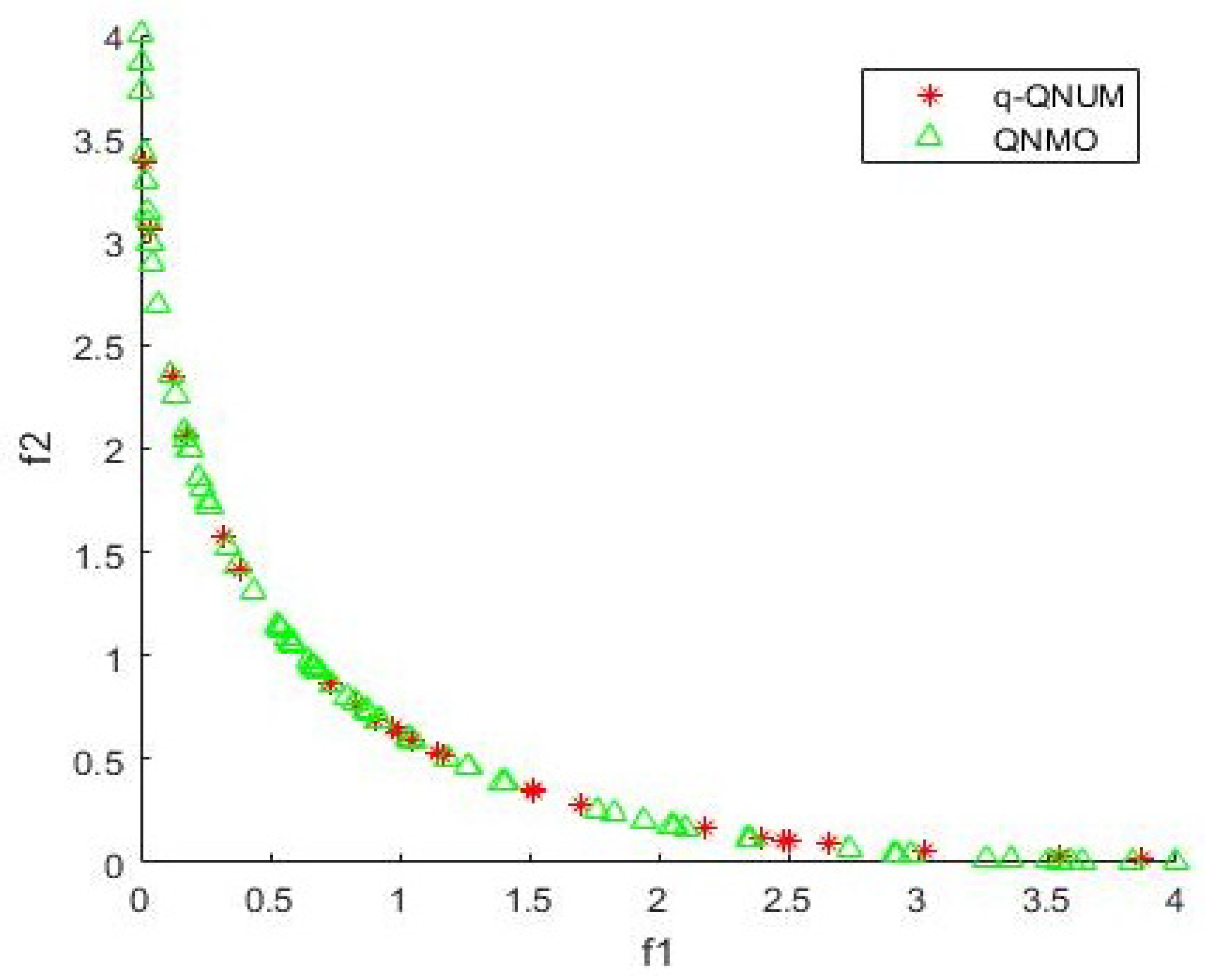
5. Numerical Results

The proposed algorithm (q-QNUM), i.e., Algorithm 2, presented in Section 4 is implemented in MATLAB (2017a) and tested on some test problems known from the literature. All tests were run under the same conditions. The box constraints of the form $lb\le x\le ub$ are used for each test problem. These constraints are considered under the direction search problem (CQOP) such that the newly generated point always lies in the same box, that is, $lb\le x+d_q\le ub$ holds. We use the stopping criteria at $x^k$ as: $\psi \left(x^k\right)>-ϵ$ where $ϵ\in {\mathbb{R}}_{+}$. All test problems given in Table 1 are solved 100 times. The starting points are randomly chosen from a uniform distribution between $lb$ and $ub$. The first column in the given table is the name of the test problem. We use the abbreviation of author’s names and number of the problem in the corresponding paper. The second column indicates the source of the paper. The third column is for lower bound and upper bound. We compare the results of (q-QNUM) with (QNMO) of [40] in the form of a number of iterations ($iter$), number of objective functions evaluation ($obj$), and number of gradient evaluations ($grad$), respectively. From Table 1, we can conclude that our algorithm shows better performance.

Table 1. Numerical Results of Test Problems.

Problem	Source	[lb,ub]	(q-QNUM)			(QNMO)
			$\mathit{iter}$	$\mathit{obj}$	$\mathit{grad}$	$\mathit{iter}$	$\mathit{obj}$	$\mathit{grad}$
BK1	[46]	[−5, 10]	200	200	200	200	200	200
MOP5	[46]	[−30, 30]	141	965	612	333	518	479
MOP6	[46]	[0, 1]	250	2177	1712	181	2008	2001
MOP7	[46]	[−400, 400]	200	200	200	751	1061	1060
DG01	[47]	[−10, 13]	175	724	724	164	890	890
IKK1	[47]	[−50, 50]	170	170	170	253	254	253
SP1	[45]	[−3, 2]	200	200	200	525	706	706
SSFYY1	[45]	[−2, 2]	200	200	200	200	300	300
SSFYY2	[45]	[−100, 100]	263	277	277	263	413	413
SK1	[48]	[−10, 10]	139	1152	1152	87	732	791
SK2	[48]	[−3, 11]	154	1741	1320	804	1989	1829
VU1	[49]	[−3, 3]	316	1108	1108	11,361	19,521	11,777
VU2	[49]	[−3, 7]	99	1882	1882	100	1900	1900
VFM1	[50]	[−2, 2]	195	195	195	195	290	290
VFM2	[50]	[−4, 4]	200	200	200	524	693	678
VFM3	[50]	[−3, 3]	161	1130	601	690	1002	981

Example 2.

Find the approximate Pareto front using (q-QNUM) and (QNMO) for the given (UMOP) [45]:

$$\begin{array}{cc}\hfill \mathit{Minimize}{f}_1(x_1,x_2)& ={(x_1-1)}^2+{(x_1-x_2)}^2,\hfill \\ \hfill \mathit{Minimize}{f}_2(x_1,x_2)& ={(x_2-3)}^2+{(x_1-x_2)}^2,\hfill \end{array}$$

where $-3\le x_1,x_2\le 10$.

The number of Pareto points generated due to (q-QNUM) with Algorithm 1 and (QNMO) is shown in Figure 1. One can observe that the number of iterations as $iter=200$ in (q-QNUM) and $iter=525$ in (QNMO) are responsible for generating the approximate Pareto front of above (UMOP).

Figure 1. Approximate Pareto Front of Example 1.

6. Conclusions

The q-Quasi-Newton method converges superlinearly to the solution of (UMOP) if all objective functions are strongly convex within the context of q-derivative. In a neighborhood of this solution, the algorithm uses a full Armijo steplength. The numerical performance of the proposed algorithm is faster than their actual evaluation.

References

1. Eschenauer, H.; Koski, J.; Osyczka, A. Multicriteria Design Optimization: Procedures and Applications; Springer: Berlin, Germany, 1990. [Google Scholar]
2. Haimes, Y.Y.; Hall, W.A.; Friedmann, H.T. Multiobjective Optimization in Water Resource Systems; Elsevier Scientific: Amsterdam, The Netherlands, 1975. [Google Scholar]
3. Nwulu, N.I.; Xia, X. Multi-objective dynamic economic emission dispatch of electric power generation integrated with game theory based demand response programs. Energy Convers. Manag. 2015, 89, 963–974. [Google Scholar] [CrossRef]
4. Badri, M.A.; Davis, D.L.; Davis, D.F.; Hollingsworth, J. A multi-objective course scheduling model: Combining faculty preferences for courses and times. Comput. Oper. Res. 1998, 25, 303–316. [Google Scholar] [CrossRef] [Green Version]
5. Ishibuchi, H.; Nakashima, Y.; Nojima, Y. Performance evaluation of evolutionary multiobjective optimization algorithms for multiobjective fuzzy genetics-based machine learning. Soft Comput. 2011, 15, 2415–2434. [Google Scholar] [CrossRef]
6. Liu, S.; Vicente, L.N. The stochastic multi-gradient algorithm for multi-objective optimization and its application to supervised machine learning. arXiv 2019, arXiv:1907.04472. [Google Scholar]
7. Tavana, M. A subjective assessment of alternative mission architectures for the human exploration of mars at NASA using multicriteria decision making. Comput. Oper. Res. 2004, 31, 1147–1164. [Google Scholar] [CrossRef]
8. Gass, S.; Saaty, T. The computational algorithm for the parametric objective function. Nav. Res. Logist. Q. 1955, 2, 39–45. [Google Scholar] [CrossRef]
9. Miettinen, K. Nonlinear Multiobjective Optimization; Kluwer Academic: Boston, MA, USA, 1999. [Google Scholar]
10. Fishbum, P.C. Lexicographic orders, utilities and decision rules: A survey. Manag. Sci. 1974, 20, 1442–1471. [Google Scholar] [CrossRef] [Green Version]
11. Coello, C.A. An updated survey of GA-based multiobjective optimization techniques. ACM Comput. Surv. (CSUR) 2000, 32, 109–143. [Google Scholar] [CrossRef]
12. Fliege, J.; Svaiter, B.F. Steepest descent method for multicriteria optimization. Math. Method. Oper. Res. 2000, 51, 479–494. [Google Scholar] [CrossRef]
13. Drummond, L.M.G.; Iusem, A.N. A projected gradient method for vector optimization problems. Comput. Optim. Appl. 2004, 28, 5–29. [Google Scholar] [CrossRef]
14. Drummond, L.M.G.; Svaiter, B.F. A steepest descent method for vector optimization. J. Comput. Appl. Math. 2005, 175, 395–414. [Google Scholar] [CrossRef] [Green Version]
15. Branke, J.; Dev, K.; Miettinen, K.; Slowiński, R. (Eds.) Multiobjective Optimization: Interactive and Evolutionary Approaches; Springer: Berlin, Germany, 2008. [Google Scholar]
16. Mishra, S.K.; Ram, B. Introduction to Unconstrained Optimization with R; Springer Nature: Singapore, 2019; pp. 175–209. [Google Scholar]
17. Fliege, J.; Drummond, L.M.G.; Svaiter, B.F. Newton’s method for multiobjective optimization. SIAM J. Optim. 2009, 20, 602–626. [Google Scholar] [CrossRef] [Green Version]
18. Chuong, T.D. Newton-like methods for efficient solutions in vector optimization. Comput. Optim. Appl. 2013, 54, 495–516. [Google Scholar] [CrossRef]
19. Qu, S.; Liu, C.; Goh, M.; Li, Y.; Ji, Y. Nonsmooth Multiobjective Programming with Quasi-Newton Methods. Eur. J. Oper. Res. 2014, 235, 503–510. [Google Scholar] [CrossRef]
20. Jiménez, M.A.; Garzón, G.R.; Lizana, A.R. (Eds.) Optimality Conditions in Vector Optimization; Bentham Science Publishers: Sharjah, UAE, 2010. [Google Scholar]
21. Al-Saggaf, U.M.; Moinuddin, M.; Arif, M.; Zerguine, A. The q-least mean squares algorithm. Signal Process. 2015, 111, 50–60. [Google Scholar] [CrossRef]
22. Aral, A.; Gupta, V.; Agarwal, R.P. Applications of q-Calculus in Operator Theory; Springer: New York, NY, USA, 2013. [Google Scholar]
23. Rajković, P.M.; Marinković, S.D.; Stanković, M.S. Fractional integrals and derivatives in q-calculus. Appl. Anal. Discret. Math. 2007, 1, 311–323. [Google Scholar]
24. Gauchman, H. Integral inequalities in q-calculus. Comput. Math. Appl. 2004, 47, 281–300. [Google Scholar] [CrossRef] [Green Version]
25. Bangerezako, G. Variational q-calculus. J. Math. Anal. Appl. 2004, 289, 650–665. [Google Scholar] [CrossRef] [Green Version]
26. Abreu, L. A q-sampling theorem related to the q-Hankel transform. Proc. Am. Math. Soc. 2005, 133, 1197–1203. [Google Scholar] [CrossRef]
27. Koornwinder, T.H.; Swarttouw, R.F. On q-analogues of the Fourier and Hankel transforms. Trans. Am. Math. Soc. 1992, 333, 445–461. [Google Scholar]
28. Ernst, T. A Comprehensive Treatment of q-Calculus; Springer: Basel, Switzerland; Heidelberg, Germany; New York, NY, USA; Dordrecht, The Netherlands; London, UK, 2012. [Google Scholar]
29. Noor, M.A.; Awan, M.U.; Noor, K.I. Some quantum estimates for Hermite-Hadamard inequalities. Appl. Math. Comput. 2015, 251, 675–679. [Google Scholar] [CrossRef]
30. Pearce, C.E.M.; Pec̆arić, J. Inequalities for differentiable mappings with application to special means and quadrature formulae. Appl. Math. Lett. 2000, 13, 51–55. [Google Scholar] [CrossRef] [Green Version]
31. Ernst, T. A Method for q-Calculus. J. Nonl. Math. Phys. 2003, 10, 487–525. [Google Scholar] [CrossRef] [Green Version]
32. Sterroni, A.C.; Galski, R.L.; Ramos, F.M. The q-gradient vector for unconstrained continuous optimization problems. In Operations Research Proceedings; Hu, B., Morasch, K., Pickl, S., Siegle, M., Eds.; Springer: Heidelberg, Germany, 2010; pp. 365–370. [Google Scholar]
33. Gouvêa, E.J.C.; Regis, R.G.; Soterroni, A.C.; Scarabello, M.C.; Ramos, F.M. Global optimization using q-gradients. Eur. J. Oper. Res. 2016, 251, 727–738. [Google Scholar] [CrossRef]
34. Chakraborty, S.K.; Panda, G. Newton like line search method using q-calculus. In International Conference on Mathematics and Computing. Communications in Computer and Information Science; Giri, D., Mohapatra, R.N., Begehr, H., Obaidat, M., Eds.; Springer: Singapore, 2017; Volume 655, pp. 196–208. [Google Scholar]
35. Mishra, S.K.; Panda, G.; Ansary, M.A.T.; Ram, B. On q-Newton’s method for unconstrained multiobjective optimization problems. J. Appl. Math. Comput. 2020. [Google Scholar] [CrossRef]
36. Jackson, F.H. On q-functions and a certain difference operator. Earth Environ. Sci. Trans. R. Soc. Edinb. 1908, 46, 253–281. [Google Scholar] [CrossRef]
37. Bento, G.C.; Neto, J.C. A subgradient method for multiobjective optimization on Riemannian manifolds. J. Optimiz. Theory App. 2013, 159, 125–137. [Google Scholar] [CrossRef]
38. Andrei, N. A diagonal quasi-Newton updating method for unconstrained optimization. Numer. Algorithms 2019, 81, 575–590. [Google Scholar] [CrossRef]
39. Nocedal, J.; Wright, S.J. Numerical Optimization, 2nd ed.; Springer Series in Operations Research and Financial Engineering; Springer: New York, NY, USA, 2006. [Google Scholar]
40. Povalej, Z. Quasi-Newton’s method for multiobjective optimization. J. Comput. Appl. Math. 2014, 255, 765–777. [Google Scholar] [CrossRef]
41. Ye, Y.L. D-invexity and optimality conditions. J. Math. Anal. Appl. 1991, 162, 242–249. [Google Scholar] [CrossRef] [Green Version]
42. Morovati, V.; Basirzadeh, H.; Pourkarimi, L. Quasi-Newton methods for multiobjective optimization problems. 4OR-Q. J. Oper. Res. 2018, 16, 261–294. [Google Scholar] [CrossRef]
43. Samei, M.E.; Ranjbar, G.K.; Hedayati, V. Existence of solutions for equations and inclusions of multiterm fractional q-integro-differential with nonseparated and initial boundary conditions. J. Inequal Appl. 2019, 273. [Google Scholar] [CrossRef] [Green Version]
44. Adams, C.R. The general theory of a class of linear partial difference equations. Trans. Am. Math.Soc. 1924, 26, 183–312. [Google Scholar]
45. Sefrioui, M.; Perlaux, J. Nash genetic algorithms: Examples and applications. In Proceedings of the 2000 Congress on Evolutionary Computation, La Jolla, CA, USA, 16–19 July 2000; Volume 1, pp. 509–516. [Google Scholar]
46. Huband, S.; Hingston, P.; Barone, L.; While, L. A review of multiobjective test problems and a scalable test problem toolkit. IEEE T. Evolut. Comput. 2006, 10, 477–506. [Google Scholar] [CrossRef] [Green Version]
47. Ikeda, K.; Kita, H.; Kobayashi, S. Failure of Pareto-based MOEAs: Does non-dominated really mean near to optimal? In Proceedings of the 2001 Congress on Evolutionary Computation, Seoul, Korea, 27–30 May 2001; Volume 2, pp. 957–962. [Google Scholar]
48. Shim, M.B.; Suh, M.W.; Furukawa, T.; Yagawa, G.; Yoshimura, S. Pareto-based continuous evolutionary algorithms for multiobjective optimization. Eng Comput. 2002, 19, 22–48. [Google Scholar] [CrossRef] [Green Version]
49. Valenzuela-Rendón, M.; Uresti-Charre, E.; Monterrey, I. A non-generational genetic algorithm for multiobjective optimization. In Proceedings of the Seventh International Conference on Genetic Algorithms, East Lansing, MI, USA, 19–23 July 1997; pp. 658–665. [Google Scholar]
50. Vlennet, R.; Fonteix, C.; Marc, I. Multicriteria optimization using a genetic algorithm for determining a Pareto set. Int. J. Syst. Sci. 1996, 27, 255–260. [Google Scholar] [CrossRef]