Multi-Partitions Subspace Clustering

Abstract

In model based clustering, it is often supposed that only one clustering latent variable explains the heterogeneity of the whole dataset. However, in many cases several latent variables could explain the heterogeneity of the data at hand. Finding such class variables could result in a richer interpretation of the data. In the continuous data setting, a multi-partition model based clustering is proposed. It assumes the existence of several latent clustering variables, each one explaining the heterogeneity of the data with respect to some clustering subspace. It allows to simultaneously find the multi-partitions and the related subspaces. Parameters of the model are estimated through an EM algorithm relying on a probabilistic reinterpretation of the factorial discriminant analysis. A model choice strategy relying on the BIC criterion is proposed to select to number of subspaces and the number of clusters by subspace. The obtained results are thus several projections of the data, each one conveying its own clustering of the data. Model’s behavior is illustrated on simulated and real data.

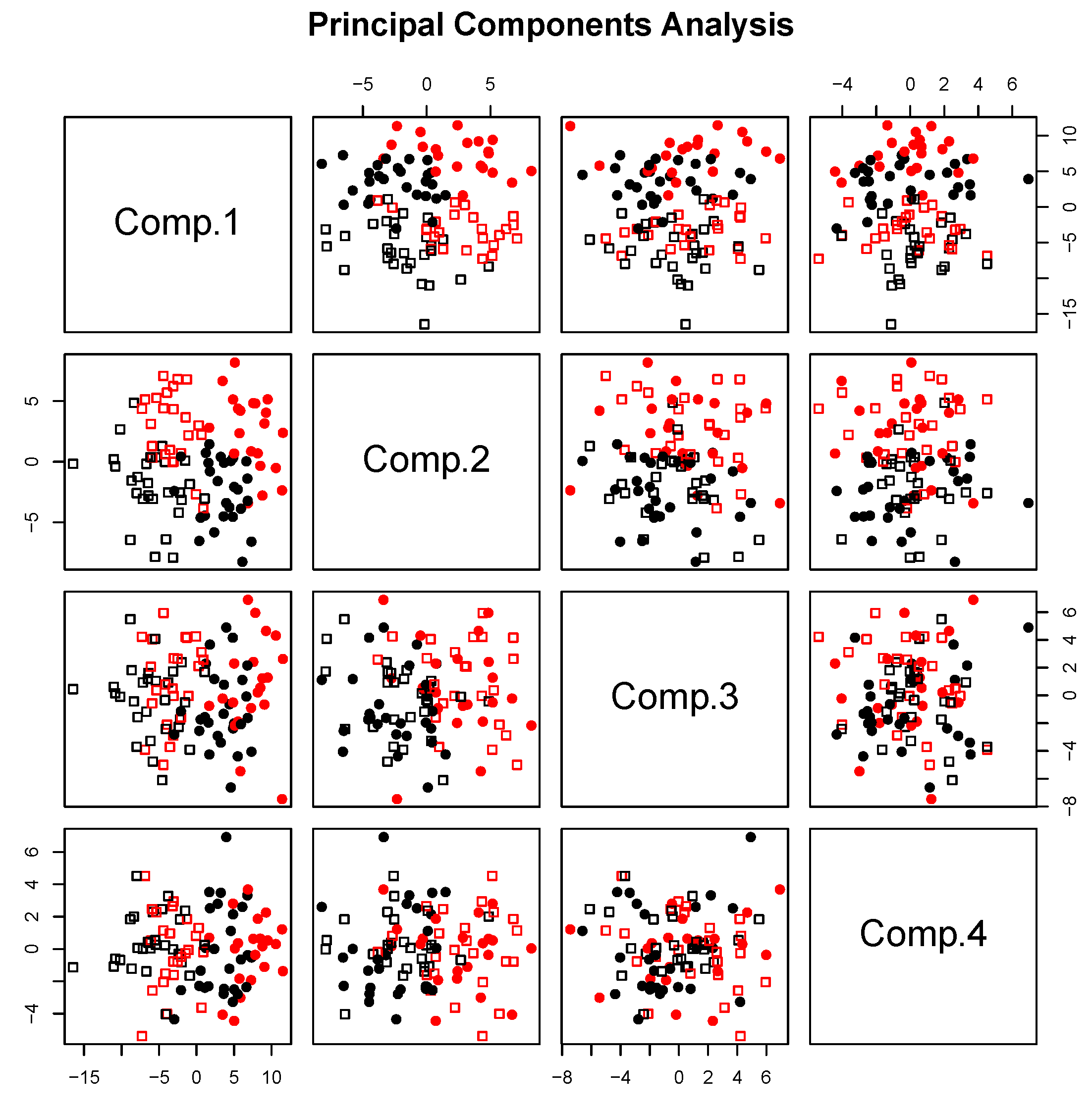
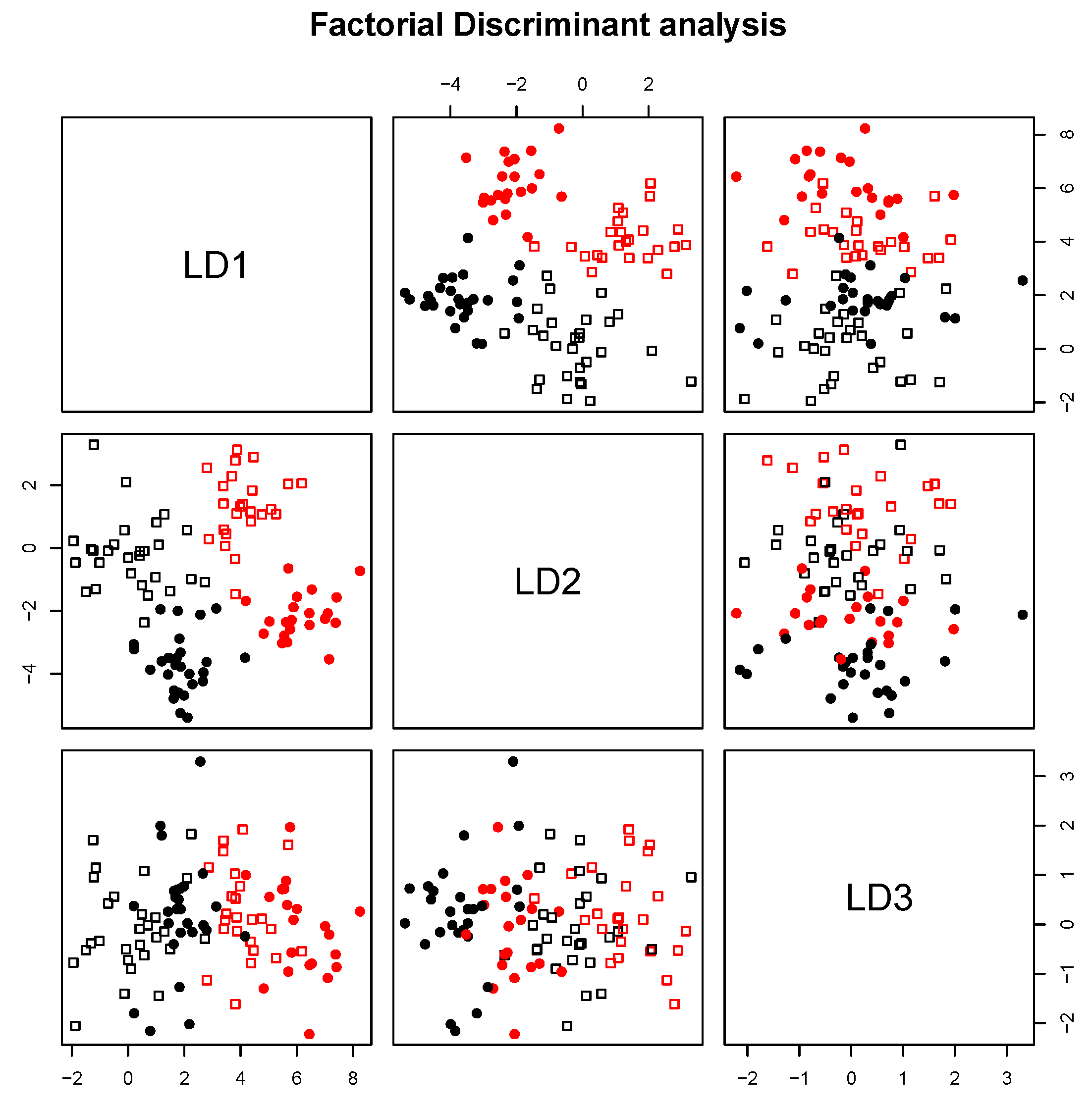
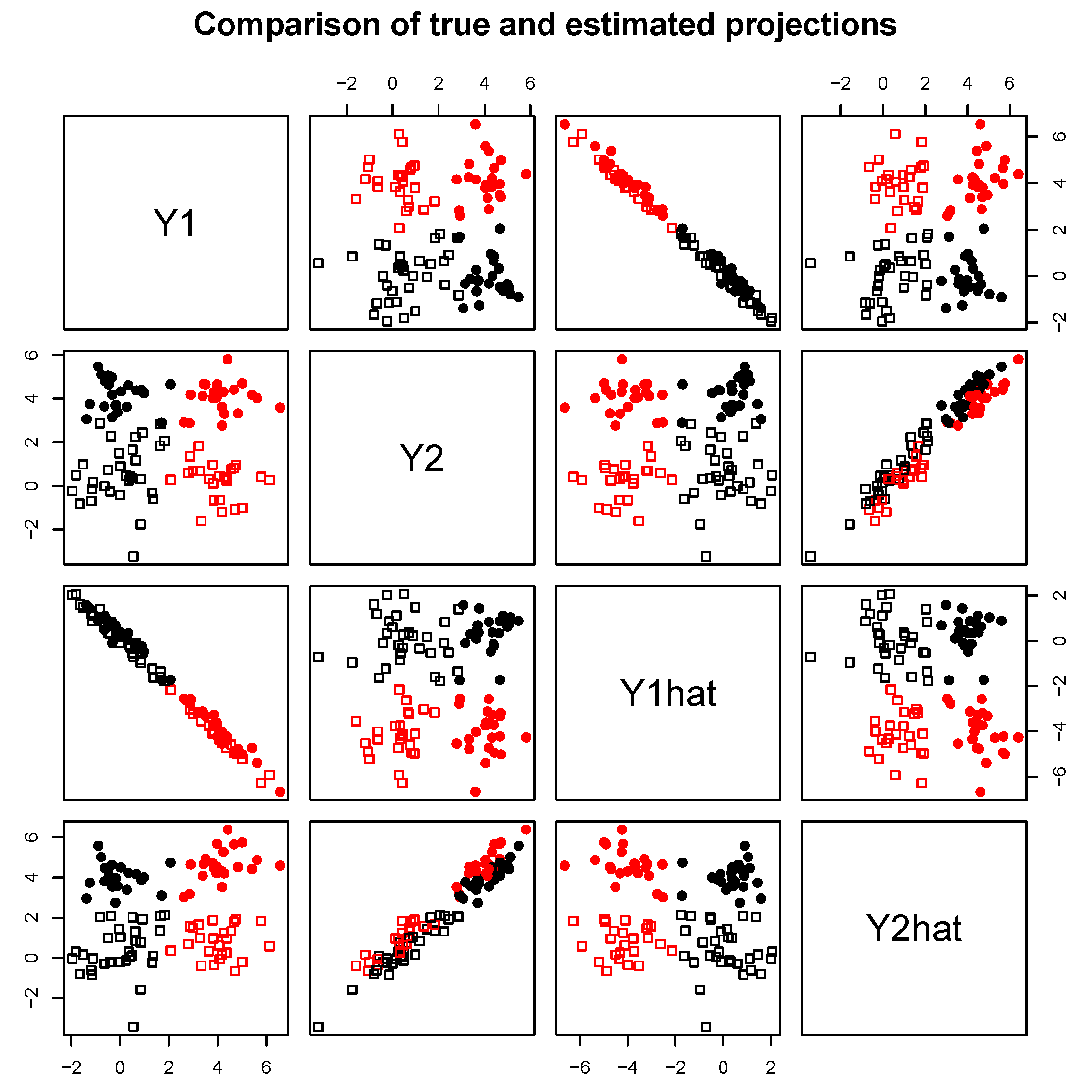
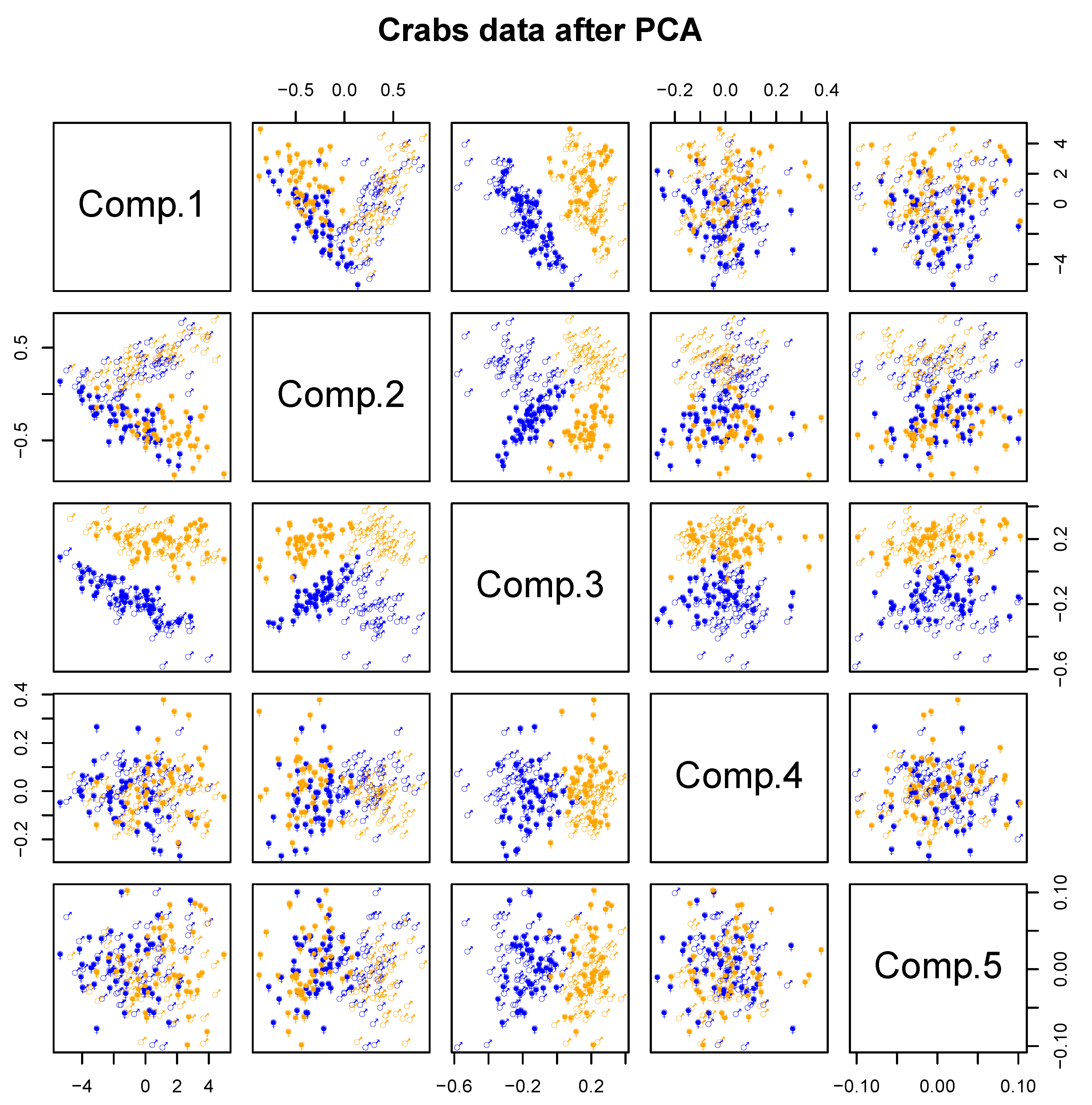
1. Introduction

In exploratory data analysis, the statistician often uses clustering and visualization in order to improve his knowledge on the data. In visualization he looks for some principal components explaining some major characteristics of the data. For example in principal component analysis (PCA) the goal is to find a linear combination of the variables explaining the major variability of the data. In cluster analysis, the goal is to find some clusters explaining the major heterogeneity of the data. In this article we suppose that the data can contain several clustering latent variables, that is, we are in the multiple partition setting, and we are simultaneously looking for clustering subspaces, that is, linear projections of the data each one related to some clustering latent variable thus the developed model is later called multi-partitions subspace clustering. A solution to perform multi-partition subspace clustering is to use a probabilistic model on the data such as a mixture model [1], it allows to perform the parameters estimation, and model selection such as the choice of the number of subspaces and the number of clusters per subspace using standard model choice criteria such as BIC [2]. Thus the main fields related to our work are model based subspace clustering and multi-partitions clustering.

In the model based subspace clustering framework, let first notice that PCA can be re-interpreted in a probabilistic way by considering a parsimonious version of a multivariate Gaussian distribution [3] and that the k-means algorithm can be re-interpreted as a particular parsimonious Gaussian mixture model estimated using a classification EM algorithm [4]. A re-interpretation of the probabilistic PCA has also been used in clustering by Bouveyron et al. [5] in order to cluster high-dimensional data. Although the proposed high dimensional mixture does not performs dimension reduction, it rather operates a class per class dimension reduction which does not allow to have a global model-based data visualization. Thus Bouveyron and Brunet [6] proposed the so called Fisher-EM algorithm which simultaneously performs clustering and dimension reduction. This is performed through a modified version of the EM algorithm [7] by including a Fisher step between the E and the M step. This approach allows the same projection to be applied to all data, but does not guarantee the increasing of the likelihood at each iteration of the algorithm.

In the context of multi-partitions clustering, Galimberti and Soffritti [8] assumed that the variables can be partitioned into several independent blocks, each one following a full-covariance Gaussian mixture model. The model selection was done by maximizing the BIC criterion by a forward/backward approach. Then, Galimberti et al. [9] generalized thier previous work by relaxing the assumption of block independence. The proposed extension takes into account three types of variables, classifying variables, redundant variables and non-classifying variables. In this context, the choice of the model is difficult because several roles have to be taken into account for each variable, which requires a lot of calculations, even for the reallocation of only one variable. Poon et al. [10] also took into account the multi-partition setting, called as facet determination in their article. The model considered is similar to that of Galimberti and Soffritti [8], but it also allows tree dependency between latent class variables, resulting in the Pouch Latent Tree Models (PLTM). Model selection is performed by a greed search to maximize the BIC criterion. The resulting model allows a broad understanding of the data, but the tree structure search makes estimation even more difficult as the number of variables increases. More recently, Marbac and Vandewalle [11] proposed a tractable muti-partition clustering algorithm not limited to continuous data; in the Gaussian setting it can be seen as particular case of Galimberti and Soffritti [8] where they assume a diagonal covariance matrix allowing a particularly efficient search of the partition of the variables in sub-vectors.

In this article we suppose that the data can contain several clustering latent variables, that is we are in the multiple partition setting. But contrary to Marbac and Vandewalle [11] where it is assumed that variables are divided into blocks each one related to some clustering of the data, we are looking for clustering subspaces, i.e., linear projections of the data each one related to some particular clustering latent variable thus replacing the combinatorial question of finding the partition of the variables in independent sub-vectors by the question of finding the coefficients of the linear combinations. The proposed approach can be related to the independent factor analysis [12] where the author deals with source separation, in our framework a source can be interpreted as some specific clustering subspace; however, their approach becomes intractable as the numbers of sources increases and does not allow to consider multivariate subspaces. Moreover, it is not invariant up to a rotation and rescaling of the data, where our proposed methodology is.

The organisation of the paper is the following, in Section 2 we present a reinterpretation of the factorial discriminant analysis as a search of discriminant components and of independent non-discriminant components. In Section 3, the multi-partitions subspace clustering model and the EM algorithm to estimate the parameters of the model will be presented. In Section 4, results on simulated and real data will show the interest of the method in practice. In Section 5, a conclusion and discussion of future extension of the paper will be made.

2. Probabilistic Interpretation of the Factorial Discriminant Analysis

2.1. Linear Discriminant Analysis (LDA)

It is supposed that n quantitative data in dimension d are available, the data number i will be denoted by ${\mathit{x}}_i={(x_{i1},\dots ,x_{id})}^{\mathrm{T}}$, where $x_{ij}$ is the value of variable j of data i. The whole dataset will be denoted by $\mathbf{x}={({\mathit{x}}_1,\dots ,{\mathit{x}}_n)}^{\mathrm{T}}$. Let assume that the data is clustered in K clusters, the class label of data i will be denoted by ${\mathit{z}}_i={(z_{i1},\dots ,z_{iK})}^{\mathrm{T}}$, with $z_{ik}$ equals to 1 if data i belongs to cluster k and 0 otherwise. Let also denote by $\mathbf{z}=({\mathit{z}}_1,\dots ,{\mathit{z}}_n)$ the partition of $\mathbf{x}$. In this section $\mathbf{z}$ is supposed to be known. For sake of simplicity the random variables and their realisations will be denoted in lower case, and p will be used as a generic notation to denote a probability distribution function (p.d.f.) which will be interpreted according to its arguments.

In the context of linear discriminant analysis [13], it is supposed that the distribution ${\mathit{x}}_i$ given the cluster follows a d-variate Gaussian distribution with common covariance matrices:

$$\forall k\in \{1,\dots ,K\},{\mathit{x}}_i|z_{ik}=1\sim {\mathcal{N}}_d({\mathit{\mu }}_k,\mathbf{\Sigma }),$$

with ${\mathit{\mu }}_k$ the vector of means in cluster k and $\mathbf{\Sigma }$ the common class conditional covariance matrix. Let also denote by ${\pi }_k=p(z_{ik}=1)$ the prior weights of each cluster.

The posterior cluster membership probabilities can be computed using the Bayes formula:

$$p(z_{ik}=1|{\mathit{x}}_i)=\frac{{\pi }_k{\varphi }_d({\mathit{x}}_i;{\mathit{\mu }}_k,\mathbf{\Sigma })}{{\sum }_{k^{\prime }=1}^K{\pi }_{k^{\prime }}{\varphi }_d({\mathit{x}}_i;{\mathit{\mu }}_{k^{\prime }},\mathbf{\Sigma })},$$

(1)

where ${\varphi }_d(·;{\mathit{\mu }}_k,\mathbf{\Sigma })$ stands for the p.d.f. of the d-variable Gaussian distribution with expectation ${\mathit{\mu }}_k$ and covariance matrix $\mathbf{\Sigma }$.

Let ${\overline{\mathit{x}}}_k$ denote the class conditional mean in cluster k:

$${\overline{\mathit{x}}}_k=\frac{1}{n_k}\sum _{i=1}^n{z}_{ik}{\mathit{x}}_i,$$

with $n_k={\sum }_{i=1}^n{z}_{ik}$ the number of data in cluster k, and by $\overline{\mathit{x}}$ the unconditional mean. Let also denote by $\mathit{W}$ the empirical intra-class covariance matrix:

$$\mathit{W}=\frac{1}{n}\sum _{k=1}^K\sum _{i=1}^n{z}_{ik}({\mathit{x}}_i-{\overline{\mathit{x}}}_k){({\mathit{x}}_i-{\overline{\mathit{x}}}_k)}^{\mathrm{T}},$$

and by $\mathit{B}$ the empirical between class covariance matrix:

$$\mathit{B}=\frac{1}{n}\sum _{k=1}^K{n}_k({\overline{\mathit{x}}}_k-\overline{\mathit{x}}){({\overline{\mathit{x}}}_k-\overline{\mathit{x}})}^{\mathrm{T}}.$$

If the data are supposed to be independent, the likelihood can simply be written as:

$$\begin{array}{cc}\hfill \ell ({\pi }_1,\dots ,{\pi }_K,{\mathit{\mu }}_1,\dots ,{\mathit{\mu }}_K,\mathbf{\Sigma };\mathbf{x},\mathbf{z})=& -\frac{n}{2}log(det(\mathbf{\Sigma }))-\frac{1}{2}\sum _{i=1}^n\sum _{k=1}^K{z}_{ik}{\parallel {\mathit{x}}_i-{\mathit{\mu }}_k\parallel }_{{\mathbf{\Sigma }}^{-1}}^2\hfill \\ & +\sum _{i=1}^n\sum _{k=1}^K{z}_{ik}log\left({\pi }_k\right)-\frac{n}{2}log\left(2\pi \right).\hfill \end{array}$$

The maximum likelihood estimators of the parameters of ${\pi }_k$, ${\mathit{\mu }}_k$ and $\mathbf{\Sigma }$ are ${\widehat{\pi }}_k=\frac{n_k}{n}$, ${\widehat{\mathit{\mu }}}_k={\overline{\mathit{x}}}_k$ and $\widehat{\mathbf{\Sigma }}=\mathit{W}$. A new data point can be then classified by plugin the estimated values of the parameters in Equation (1):

$${\widehat{\mathit{z}}}_i=\underset{k\in \{1,\dots ,K\}}{argmax}{\widehat{\mathit{\mu }}}_k^{\mathrm{T}}{\widehat{\mathbf{\Sigma }}}^{-1}{\mathit{x}}_i-\frac{1}{2}{\mathit{\mu }}_k^{\mathrm{T}}{\widehat{\mathbf{\Sigma }}}^{-1}{\mathit{\mu }}_k+log\left({\widehat{\pi }}_k\right),$$

the resulting classification boundary being linear in this case.

2.2. Factorial Discriminant Analysis (FDA)

Let us note that, from a descriptive viewpoint, one can be interested in dimension reduction in order to visualize the data. This could be done by using PCA, but from a classification perspective the component explaining the largest variability in the data are often not the same that the components providing the best separation between the clusters.

The goal of factorial discriminant analysis (FDA) is to find the component maximizing the variance explained by the cluster above the intra-class variance. The coefficients of the first discriminant component ${\mathit{v}}_1\in {\mathbb{R}}^d$ is defined by

$${\mathit{v}}_1=arg\underset{\mathit{v}\in {\mathbb{R}}^d}{max}\frac{{\mathit{v}}^{\mathrm{T}}\mathit{B}\mathit{v}}{{\mathit{v}}^{\mathrm{T}}\mathit{W}\mathit{v}}.$$

It is well known that ${\mathit{v}}_1$ is the eigen vector associated with the highest eigen value ${\lambda }_1$ of ${\mathit{W}}^{-1}\mathit{B}$ [14]. The remaining discriminant components are obtained through the remaining eigen vectors of ${\mathit{W}}^{-1}\mathit{B}$. Let denote by ${\lambda }_1,\dots ,{\lambda }_{K-1}$ the eigen values of ${\mathit{W}}^{-1}\mathit{B}$ sorted in decreasing order and by ${\mathit{v}}_1,\dots ,{\mathit{v}}_{K-1}$ the associated eigen vectors. Moreover, if each component is constrained to have an intra-class variance equal to one (i.e., ${{\mathit{v}}_k}^{\mathrm{T}}\mathit{W}{\mathit{v}}_k=1$, $\forall k\in \{1,\dots ,K-1\}$), the classification obtained using the Mahalonobis distance can simply be obtained by using the Euclidean distance on the data projected on the discriminant components.

2.3. Equivalence between LDA and FDA

As proved in Campbell [15] and detailed in Trevor Hastie [16], the FDA can be interpreted in a probabilistic way as an LDA where the rank of $\{{\mathit{\mu }}_1,\dots ,{\mathit{\mu }}_K\}$ is constrained to be equal to p with $p\le K-1$ under the common class covariance matrix assumption. This allows us to reparametrize the probabilistic model in the following way:

$${\mathit{x}}_i|z_{ik}=1\sim {\mathcal{N}}_d\left(\mathit{A}\right(\begin{array}{c}{\mathit{\nu }}_k\\ \mathit{\gamma }\end{array}),\mathit{A}{\mathit{A}}^{\mathrm{T}}),$$

where ${\mathit{\nu }}_k\in {\mathbb{R}}^p$, $\mathit{\gamma }\in {\mathbb{R}}^{d-p}$ and $\mathit{A}\in {\mathcal{M}}_{d,d}\left(\mathbb{R}\right)$. Let notice that this new parametrization at this step is not unique but the model can easily be made identifiable by imposing some constraints on the parameters.

Let ${\mathit{y}}_i\in {\mathbb{R}}^p$ and ${\mathit{u}}_i\in {\mathbb{R}}^{d-p}$ two random variables, the new parametrization can be reinterpreted in the following generative framework:

• Draw ${\mathit{z}}_i$: ${\mathit{z}}_i\sim \mathcal{M}(1;{\pi }_1,\dots ,{\pi }_K)$ where $\mathcal{M}$ stands for the multinomial distribution
• Draw ${\mathit{y}}_i|{\mathit{z}}_i$: ${\mathit{y}}_i|z_{ik}=1\sim {\mathcal{N}}_p({\mathit{\nu }}_k,{\mathit{I}}_p)$
• Draw ${\mathit{u}}_i$: ${\mathit{u}}_i\sim {\mathcal{N}}_{d-p}(\mathit{\gamma },{\mathit{I}}_{d-p})$
• Compute ${\mathit{x}}_i$ based on ${\mathit{y}}_i$ and ${\mathit{u}}_i$: ${\mathit{x}}_i=\mathit{A}\left(\begin{array}{c}{\mathit{y}}_i\\ {\mathit{u}}_i\end{array}\right)$.

Thus the p.d.f. of ${\mathit{x}}_i$ can be factorized in the following way:

$$p\left({\mathit{x}}_i\right)=\frac{1}{\left|\mathit{A}\right|}p\left({\mathit{u}}_i\right)p\left({\mathit{y}}_i\right).$$

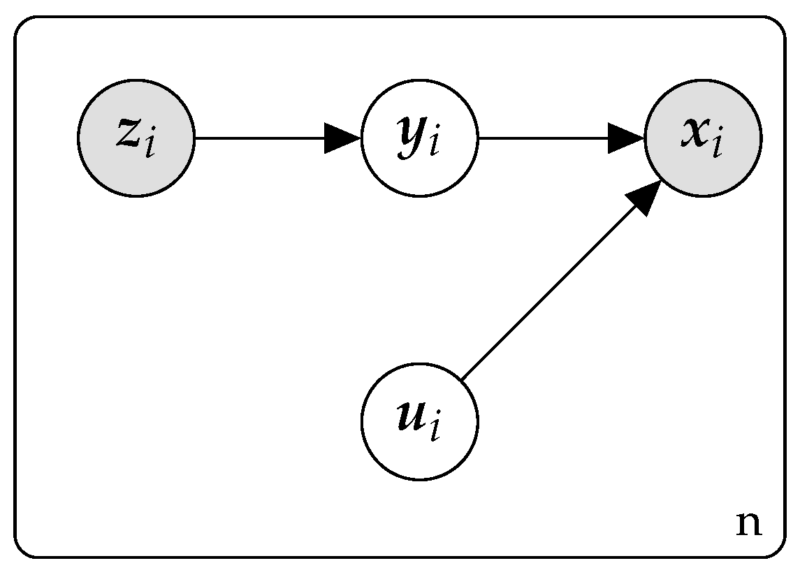
From a graphical angle the model can be reinterpreted as in Figure 1, where ${\mathit{u}}_i$ and ${\mathit{y}}_i$ are latent random variables.

In practice we are interested in finding ${\mathit{y}}_i$ and ${\mathit{u}}_i$ from ${\mathit{x}}_i$. We will denote by $\mathit{V}\in {\mathcal{M}}_{p,d}\left(\mathbb{R}\right)$ and $\mathit{R}\in {\mathcal{M}}_{d-p,d}\left(\mathbb{R}\right)$ the matrices which allow this computation: ${\mathit{y}}_i=\mathit{V}{\mathit{x}}_i$, ${\mathit{u}}_i=\mathit{R}{\mathit{x}}_i$. It is obvious that $\left(\begin{array}{c}\mathit{V}\\ \mathit{R}\end{array}\right)={\mathit{A}}^{-1}$, for the rest of the article only the parametrization in terms of $\mathit{V}$ and $\mathit{R}$ will be used.

The main interest of this parametrization is that

$$p(z_{ik}=1|{\mathit{x}}_i)=p(z_{ik}=1|{\mathit{y}}_i,{\mathit{u}}_i)=p(z_{ik}=1|{\mathit{y}}_i)=p(z_{ik}=1|\mathit{V}{\mathit{x}}_i).$$

It means that only $\mathit{V}{\mathit{x}}_i$ is required to compute the posterior class membership probabilities:

$$p(z_{ik}=1|{\mathit{x}}_i)=\frac{{\pi }_k{\varphi }_p(\mathit{V}{\mathit{x}}_i;{\mathit{\nu }}_k,{\mathit{I}}_p)}{{\sum }_{k^{\prime }=1}^K{\pi }_{k^{\prime }}{\varphi }_p(\mathit{V}{\mathit{x}}_i;{\mathit{\nu }}_{k^{\prime }},{\mathit{I}}_p)}.$$

(2)

Parameters are estimated by maximum likelihood, using the variable change formulae the likelihood can be written:

$$\begin{array}{cc}\hfill \ell ({\pi }_1,\dots ,{\pi }_K,\mathit{V},\mathit{R},\mathit{\gamma },{\mathit{\nu }}_1,\dots ,{\mathit{\nu }}_K;\mathbf{x},\mathbf{z})=& nlog\mid det\left(\begin{array}{c}\mathit{V}\\ \mathit{R}\end{array}\right)\mid -\frac{1}{2}\sum _{i=1}^n\sum _{k=1}^K{z}_{ik}{\parallel \mathit{V}{\mathit{x}}_i-{\mathit{\nu }}_k\parallel }^2\hfill \\ & +\sum _{i=1}^n\sum _{k=1}^K{z}_{ik}log\left({\pi }_k\right)-\frac{1}{2}\sum _{i=1}^n{\parallel \mathit{R}{\mathit{x}}_i-\mathit{\gamma }\parallel }^2-\frac{n}{2}log\left(2\pi \right).\hfill \end{array}$$

The first term is related to the variable change, the second term is related to the discriminant components and the third term is related to prior class membership probabilities and the fourth term is related to the non-discriminant components. In practice, this decomposition is the corner stone of the proposed approach since it separates the clustering part from the non-clustering part.

As stated in Campbell [15] the maximum likelihood estimator of $\mathit{V}$ are the first p eigen vectors ${\mathit{v}}_1,\dots ,{\mathit{v}}_p$ of ${\mathit{W}}^{-1}\mathit{B}$ in rows:

$$\widehat{\mathit{V}}=\left(\begin{array}{c}{\mathit{v}}_1^{\mathrm{T}}\\ ⋮\\ {\mathit{v}}_p^{\mathrm{T}}\end{array}\right),$$

renormalized such that:

$$\widehat{\mathit{V}}\mathit{W}{\widehat{\mathit{V}}}^{\mathrm{T}}={\mathit{I}}_p.$$

The maximum likelihood estimator of $\mathit{R}$ is obtained such that:

$$\widehat{\mathit{R}}\mathit{W}{\widehat{\mathit{V}}}^{\mathrm{T}}=0$$

and that

$$\widehat{\mathit{R}}\mathit{W}{\widehat{\mathit{R}}}^{\mathrm{T}}={\mathit{I}}_{d-p},$$

(3)

with ${\mathit{D}}_{d-p}$ the diagonal matrix of the $d-p$ last eigen-values of ${\mathit{W}}^{-1}\mathit{B}$ (with the $d-K$ last eigen-values which are null). ${\widehat{\mathit{R}}}^{\mathrm{T}}$ can simply be obtained by multiplying the last $d-p$ egien-vectors of ${\mathit{W}}^{-1/2}\mathit{B}{\mathit{W}}^{-1/2}$ by ${\mathit{W}}^{-1/2}$ then renormalize them such that Equation (3) is satisfied. Such renormalization makes the parameters V et R identifiable up to a sign.

Moreover ${\mathit{\nu }}_k$ and $\mathit{\gamma }$ are estimated by

$${\widehat{\mathit{\nu }}}_k=\frac{1}{n_k}\sum _{i=1}^n{z}_{ik}\widehat{\mathit{V}}{\mathit{x}}_i,$$

$$\widehat{\mathit{\gamma }}=\frac{1}{n}\sum _{i=1}^n\widehat{\mathit{R}}{\mathit{x}}_i.$$

As stated in Trevor Hastie [16] the link between the two parametrizations is as follows:

$${\widehat{\mathit{\mu }}}_k=\mathit{W}{\widehat{\mathit{V}}}^{\mathrm{T}}\widehat{\mathit{R}}({\overline{\mathit{x}}}_k-\overline{\mathit{x}})+\overline{\mathit{x}},$$

and

$$\widehat{\mathbf{\Sigma }}=\mathit{W}+\mathit{W}{\widehat{\mathit{R}}}^{\mathrm{T}}\widehat{\mathit{R}}\mathit{B}{\widehat{\mathit{R}}}^{\mathrm{T}}\widehat{\mathit{R}}\mathit{W}.$$

From this formula we can clearly see that the reduced rank constraint operates some regularization on the parameters estimation. Moreover, from a practical perspective the reparametrization Equation (2) is more efficient for computing the posterior class membership probabilities.

2.4. Application in the Clustering Setting

As in Trevor Hastie [16], the model can easily be used in the clustering setting using the EM algorithm to maximise the likelihood. Thus $\mathit{W}$, $\mathit{B}$, ${\overline{\mathit{x}}}_k$ are recomputed at each iteration by using their version weighted by their posterior membership probabilities.

The EM algorithm is now presented. The algorithm is first initialized with some starting value of the parameters or of the partition. Then the E step and the M step are iterated until convergence. Let ${}^{\left(r\right)}$ denote the value of the parameters at iteration r, the E and the M steps are the followings:

• E step: compute the posterior class membership probabilities.

  $$t_{ik}^{(r+1)}=\frac{{\pi }_k{\varphi }_d({\mathit{x}}_i;{\mathit{\mu }}_k^{\left(r\right)},{\mathbf{\Sigma }}^{\left(r\right)})}{{\sum }_{k^{\prime }=1}^K{\pi }_{k^{\prime }}{\varphi }_d({\mathit{x}}_i;{\mathit{\mu }}_{k^{\prime }}^{\left(r\right)},{\mathbf{\Sigma }}^{\left(r\right)})}=\frac{{\pi }_k{\varphi }_p({\mathit{y}}_i^{\left(r\right)};{\mathit{\nu }}_k^{\left(r\right)},{\mathit{I}}_p)}{{\sum }_{k^{\prime }=1}^K{\pi }_{k^{\prime }}{\varphi }_p({\mathit{y}}_i^{\left(r\right)};{\mathit{\nu }}_{k^{\prime }}^{\left(r\right)},{\mathit{I}}_p)},$$

  with ${\mathit{y}}_i^{\left(r\right)}={\mathit{V}}^{\left(r\right)}{\mathit{x}}_i$.
• M step: Compute

  $${\overline{\mathit{x}}}_k^{(r+1)}=\frac{1}{n_k^{(r+1)}}\sum _{i=1}^n{t}_{ik}^{(r+1)}{\mathit{x}}_i,$$

  $${\mathit{W}}^{(r+1)}=\frac{1}{n}\sum _{k=1}^K\sum _{i=1}^n{t}_{ik}^{(r+1)}({\mathit{x}}_i-{\overline{\mathit{x}}}_k^{(r+1)}){({\mathit{x}}_i-{\overline{\mathit{x}}}_k^{(r+1)})}^{\mathrm{T}},$$

  $${\mathit{B}}^{(r+1)}=\frac{1}{n}\sum _{k=1}^K{n}_k^{(r+1)}({\overline{\mathit{x}}}_k^{(r+1)}-\overline{\mathit{x}}){({\overline{\mathit{x}}}_k^{(r+1)}-\overline{\mathit{x}})}^{\mathrm{T}}.$$
  Then deduce ${\mathit{V}}^{(r+1)}$, ${\mathit{R}}^{(r+1)}$, ${\mathit{\nu }}_1^{(r+1)},\dots ,{\mathit{\nu }}_K^{(r+1)}$ and ${\mathit{\gamma }}^{(r+1)}$ as in the previous section using the eigenvalue decomposition of ${{\mathit{W}}^{(r+1)}}^{-1}{\mathit{B}}^{(r+1)}$.

As noticed in Trevor Hastie [16], this approach is not equivalent to performing a standard EM algorithm and then performing FDA at the end of the EM algorithm. FDA must be computed at each iteration of the EM algorithm since the posterior membership probabilities are only computed based on the p first clustering projections.

Let us also notice that the M step can be interpreted in a Fisher-M step since FDA is required. In this sense it can be interpreted as a particular version of the Fisher-EM algorithm of Bouveyron and Brunet [6]. Although the homoscedasticity could be seen as particularly constraining, it is the best framework for introducing our model in the next section, since it is easily interpretable and allows for efficient computation owing to the closed form of FDA. This limitation could be easily overcome by using rigorous extensions of the FDA in the heteroscedastic setting as in Kumar and Andreou [17]; however, the computation would be much more intensive, since in this case no closed form formula is available and an iterative algorithm would be required even for finding the best projection.

3. Multi-Partition Subspace Mixture Model

3.1. Presentation of the Model

Let us now suppose that instead of having only one class variable ${\mathit{z}}_i$ for data i, we now have H class variables ${\mathit{z}}_i^1,\dots ,{\mathit{z}}_i^H$ with $K_1,\dots ,K_H$ modalities. It is assumed that ${\mathit{z}}_i^1,\dots ,{\mathit{z}}_i^H$ are independent, with $p(z_{ik}^h=1)$ denoted by ${\pi }_k^h$. Let also denote by ${\mathit{y}}_i^h$ the variables related to the clustering variable ${\mathit{z}}_i^h$ such that:

$${\mathit{y}}_i^h|z_{ik}^h=1\sim {\mathcal{N}}_{p_h}({\mathit{\nu }}_k^h,I_{p_h})$$

and that we will denote by $p_{•}={\sum }_{h=1}^H{p}_h$.

Let us still denote by ${\mathit{u}}_i$ the non clustering variables

$${\mathit{u}}_i\sim {\mathcal{N}}_{d-p_{•}}(\gamma ,I_{d-p_{•}}).$$

Let us also define ${\mathit{x}}_i$ by:

$${\mathit{x}}_i={\left(\begin{array}{c}{\mathit{V}}_1\\ ⋮\\ {\mathit{V}}_H\\ \mathit{R}\end{array}\right)}^{-1}\left(\begin{array}{c}{\mathit{y}}_i^1\\ ⋮\\ {\mathit{y}}_i^H\\ {\mathit{u}}_i\end{array}\right).$$

Thus,

$$p\left(\mathit{x}\right)=\left|det\left(\begin{array}{c}{\mathit{V}}_1\\ ⋮\\ {\mathit{V}}_H\\ \mathit{R}\end{array}\right)\right|p\left(\mathit{u}\right)\prod _{h=1}^{H}p\left({\mathit{y}}^h\right).$$

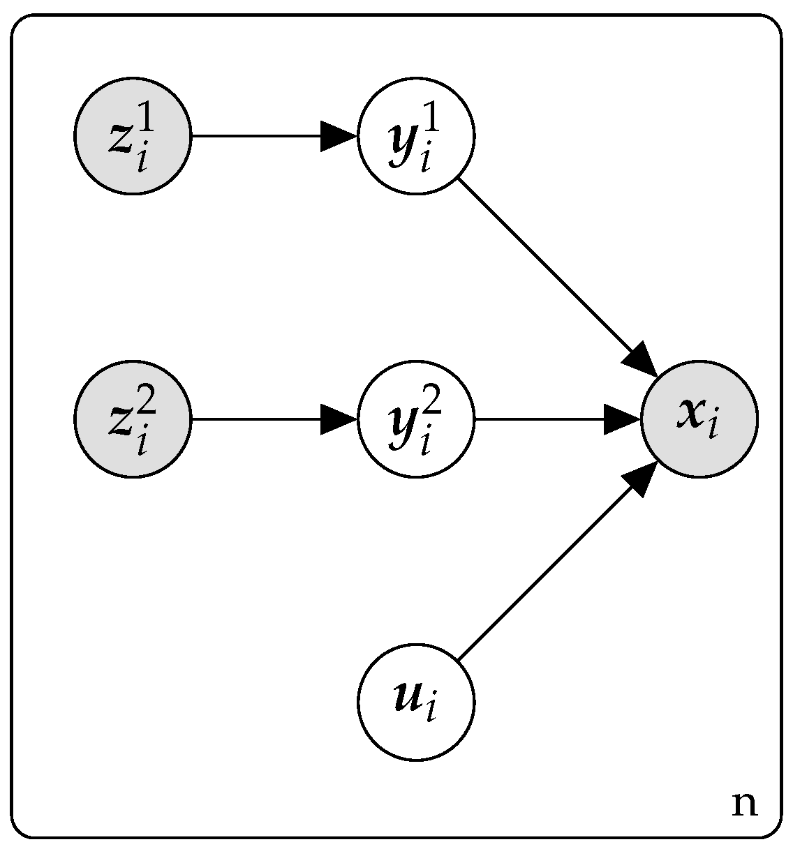
The Figure 2 illustrates the model in the case of $H=2$.

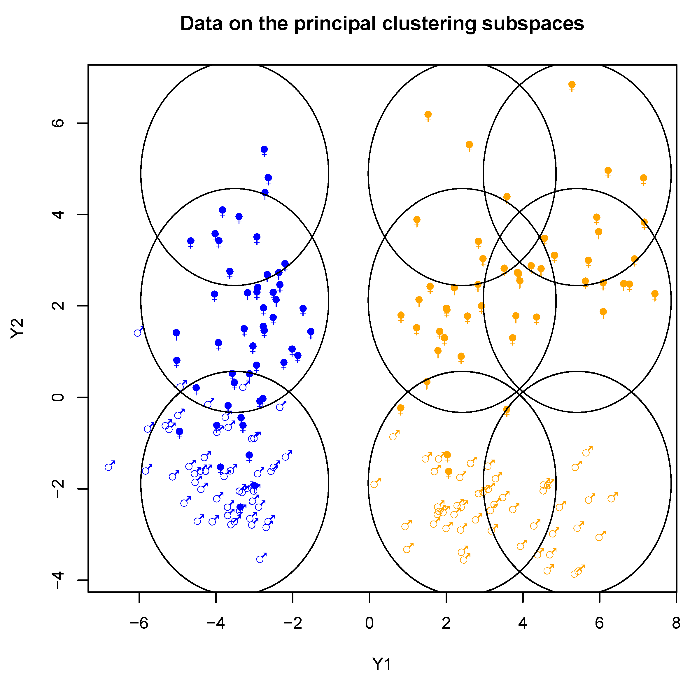
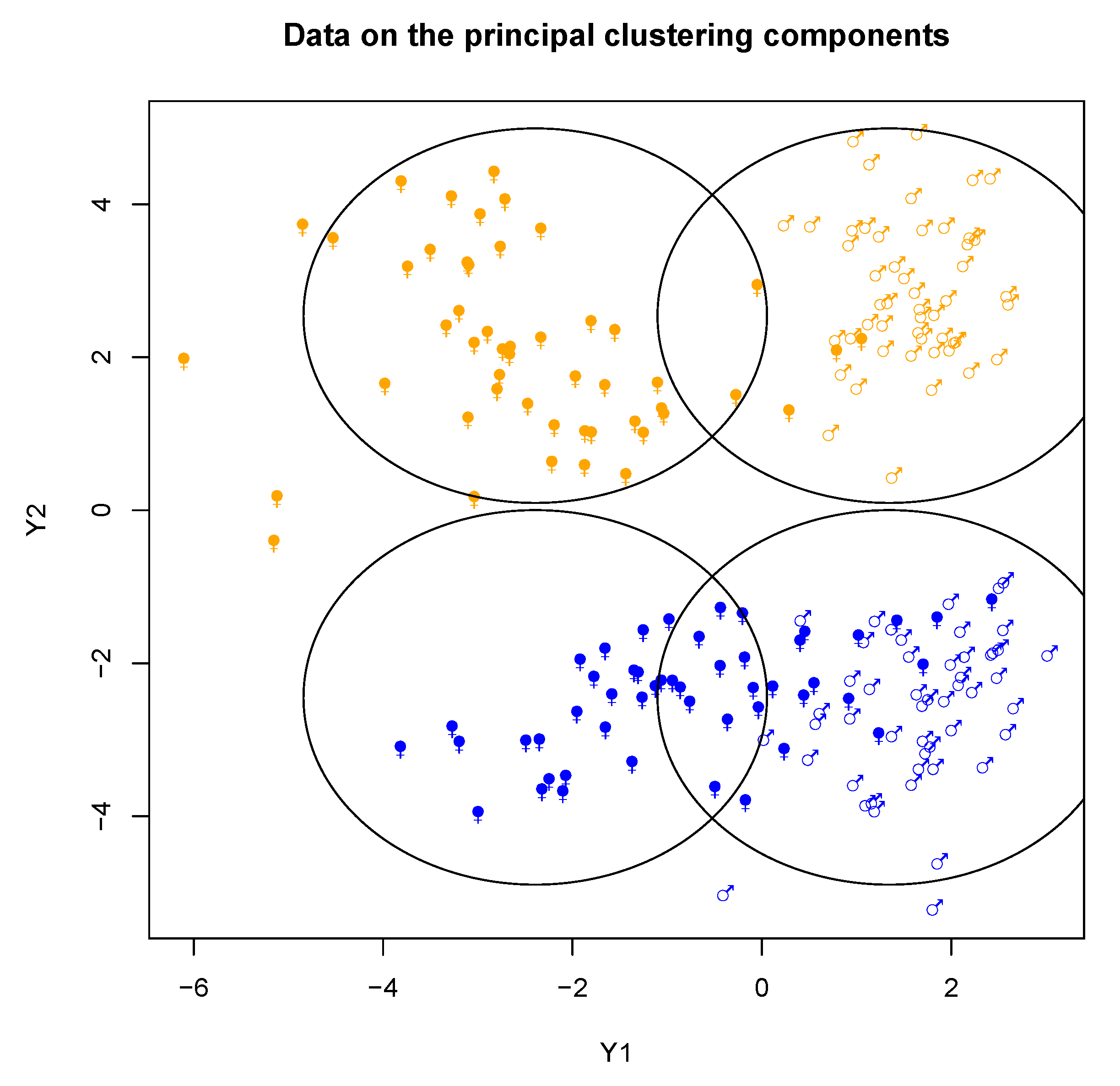
Let us notice that this model allows us to visualize many clustering viewpoints in a low dimensional space since ${\mathit{x}}_i$ can be summarized by ${\mathit{y}}_i^1$, …, ${\mathit{y}}_i^H$. For instance, one can suppose that $p_1=\dots =p_H=1$. In this case each clustering variable can be visualized on one component. We will denote by $\mathbf{\theta }=({\mathit{V}}_1,\dots ,{\mathit{V}}_H,\mathit{R},\mathit{\gamma },{\mathit{\nu }}_1^1,\dots ,{\mathit{\nu }}_{K_H}^H)$ the parameters of the model to be estimated.

3.2. Discussion about the Model

The Cartesian product of cluster spaces results in ${\prod }_{h=1}^H{K}_h$ clusters, which can be very large without needing many parameters. Thus the proposed model can be interpreted as being a very sparse Gaussian mixture model allowing the possibility to deal with a very large number of clusters, the resulting conditional means and covariances matrices are given in the following formulas:

$$\mathbb{E}({\mathit{x}}_i|z_{i{k}_1}^1=1,z_{i{k}_1}^2=1,\dots ,z_{i{k}_H}^H=1)={\left(\begin{array}{c}{\mathit{V}}_1\\ ⋮\\ {\mathit{V}}_H\\ \mathit{R}\end{array}\right)}^{-1}\left(\begin{array}{c}{\mathit{\nu }}_{k_1}^1\\ ⋮\\ {\mathit{\nu }}_{k_H}^H\\ \mathit{\gamma }\end{array}\right),$$

and

$$\mathbb{V}({\mathit{x}}_i|z_{i{k}_1}^1=1,z_{i{k}_1}^2=2,\dots ,z_{i{k}_H}^H=1)={({\mathit{V}}_1^{\mathrm{T}}{\mathit{V}}_1+\cdots +{\mathit{V}}_H^{\mathrm{T}}{\mathit{V}}_H+{\mathit{R}}^{\mathrm{T}}\mathit{R})}^{-1}.$$

Thus, the expectation of ${\mathit{x}}_i$ given in all the clusters is a linear combination of the cluster specific means which can be referred to as a multiple-way MANOVA setting. On the one hand, as a particular homoscedastic Gaussian mixture, our model is more prone to model bias than free homoscedastic Gaussian mixture, and in the case when our model would be well-specified the homoscedastic Gaussian mixture would give a similar clustering for a large sample size (i.e., the same partitions with respect to the partition resulting from the product space of our multi-partitions model). On the other hand, our approach produces a factorised version of the partition space as well as the related clustering subspaces which is not a standard output of clustering methods, and it can deal with a large number of clusters in a sparse way which can be particularly useful for a moderated sample size. In practice, the choice between our model and an other mixture model can simply be performed through the BIC criterion.

In some sense our model can be linked with the mixture of factor analyzers [18]. In mixture of factor analyzers the model is of the type:

$${\mathit{x}}_i=\mathit{A}{\mathit{y}}_i+{\mathit{u}}_i,$$

where $\mathit{A}$ is a low rank matrix. But here we have chosen a model of the type

$${\mathit{x}}_i=\mathit{A}\left(\begin{array}{c}{\mathit{y}}_i\\ {\mathit{u}}_i\end{array}\right),$$

which allows us to deal with the noise in a different way. Actually, our model is invariant up to a bijective linear transformation of the data which is not the case for the mixtures of factor analyzers. On the other hand, our model can only deal with data with moderated dimension with respect to the number of statistical units; it assumes that the sources ${\mathit{y}}_i$ can be recovered from the observed data ${\mathit{x}}_i$.

3.3. Estimation of the Parameters of the Model in the Supervised Setting

The likelihood of the model can be written:

$$\begin{array}{cc}\hfill \ell (\mathbf{\theta };\mathbf{x},\mathbf{z})=& nlog\left|det\left(\begin{array}{c}{\mathit{V}}_1\\ ⋮\\ {\mathit{V}}_H\\ \mathit{R}\end{array}\right)\right|-\sum _{i=1}^n\sum _{h=1}^H\sum _{k=1}^{K_h}{z}_{ik}^h{\parallel {\mathit{V}}_h^{\mathrm{T}}{\mathit{x}}_i-{\mathit{\nu }}_k^h\parallel }^2\hfill \\ & +\sum _{i=1}^n\sum _{h=1}^H\sum _{k=1}^{K_h}{z}_{ik}^{h}log\left({\pi }_k^h\right)-\sum _{i=1}^n{\parallel {\mathit{R}}^{\mathrm{T}}{\mathit{x}}_i-\mathit{\gamma }\parallel }^2-\frac{n}{2}log\left(2\pi \right).\hfill \end{array}$$

The likelihood cannot be maximized directly. However, in the case of $H=1$, it reduces to the problem of Section 2. Let notice that if all the parameters are fixed except ${\mathit{V}}_h$ and $\mathit{R}$, ${\mathit{\nu }}_k^h$ and $\mathit{\gamma }$, the optimisation can be easily performed by constraining ${\mathit{V}}_h^{(r+1)}$ and ${\mathit{R}}^{(r+1)}$ to be linear combinations of ${\mathit{V}}_h^{\left(r\right)}$ and ${\mathit{R}}^{\left(r\right)}$. Thus the likelihood will be optimized by using an alternate optimization algorithm. Let $\mathbf{M}\in {\mathcal{M}}_{d-p_{•}+p_h,d-p_{•}+p_h}\left(\mathbb{R}\right)$ the matrix which allow to compute ${\mathit{V}}_h^{(r+1)}$ and ${\mathit{R}}^{(r+1)}$ based on ${\mathit{V}}_h^{\left(r\right)}$ and ${\mathit{R}}^{\left(r\right)}$:

$$\left(\begin{array}{c}{\mathit{V}}_h^{(r+1)}\\ {\mathit{R}}^{(r+1)}\end{array}\right)=\mathit{M}\left(\begin{array}{c}{\mathit{V}}_h^{\left(r\right)}\\ {\mathit{R}}^{\left(r\right)}\end{array}\right)=\left(\begin{array}{c}{\mathit{M}}_1\\ {\mathit{M}}_2\end{array}\right)\left(\begin{array}{c}{\mathit{V}}_h^{\left(r\right)}\\ {\mathit{R}}^{\left(r\right)}\end{array}\right),$$

where ${\mathit{M}}_1$ is the sub-matrix containing the $p_h$ first rows of $\mathit{M}$ and ${\mathit{M}}_2$ the matrix containing the last $d-p_{•}$ rows of $\mathit{M}$.

Thus, the increase of the likelihood when all the parameters are fixed except ${\mathit{V}}_h$, $\mathit{R}$, ${\mathit{\nu }}_k^h$ and $\mathit{\gamma }$ becomes:

$$\begin{array}{cc}\hfill C({\mathit{M}}_1,{\mathit{M}}_2,{\mathit{\nu }}_k,\mathit{\gamma })=& nlog|det\left(\mathit{M}\right)|-\frac{1}{2}\sum _{i=1}^n\sum _{k=1}^{K_h}{z}_{ik}^h{∥{\mathit{M}}_1\left(\begin{array}{c}{\mathit{V}}_h^{\left(r\right)}\\ {\mathit{R}}^{\left(r\right)}\end{array}\right){\mathit{x}}_i-{\mathit{\nu }}_k^h∥}^2\hfill \\ & -\frac{1}{2}\sum _{i=1}^n{∥{\mathit{M}}_2\left(\begin{array}{c}{\mathit{V}}_h^{\left(r\right)}\\ {{\mathit{R}}^{\left(r\right)}}^{\mathrm{T}}\end{array}\right){\mathit{x}}_i-\mathit{\gamma }∥}^2.\hfill \end{array}$$

By denoting

$$\left(\begin{array}{c}{{\mathit{y}}_i^h}^{\left(r\right)}\\ {{\mathit{u}}_i}^{\left(r\right)}\end{array}\right)=\left(\begin{array}{c}{\mathit{V}}_h^{\left(r\right)}\\ {\mathit{R}}^{\left(r\right)}\end{array}\right){\mathit{x}}_i,$$

we have to maximize:

$$\begin{array}{cc}\hfill C({\mathit{M}}_1,{\mathit{M}}_2,{\mathit{\nu }}_k,\mathit{\gamma })=& nlog|det\left(\mathit{M}\right)|-\frac{1}{2}\sum _{i=1}^n\sum _{k=1}^{K_h}{z}_{ik}^h{∥{\mathit{M}}_1\left(\begin{array}{c}{{\mathit{y}}_i^h}^{\left(r\right)}\\ {{\mathit{u}}_i}^{\left(r\right)}\end{array}\right)-{\mathit{\nu }}_k^h∥}^2\hfill \\ & -\frac{1}{2}\sum _{i=1}^n{∥{\mathit{M}}_2\left(\begin{array}{c}{{\mathit{y}}_i^h}^{\left(r\right)}\\ {{\mathit{u}}_i}^{\left(r\right)}\end{array}\right)-\mathit{\gamma }∥}^2.\hfill \end{array}$$

Consequently, $\mathit{M}$ and the others parameters can be obtained by applying a simple FDA on the data $({{{\mathit{y}}_i^h}^{\left(r\right)}}^{\mathrm{T}},{{{\mathit{u}}_i}^{\left(r\right)}}^{\mathrm{T}})$. In order to optimise over all the parameters, we can loop over all the clustering dimensions.

Thus, in the case of mixed continuous and categorical data, this model can be used to visualize the clustering behavior of the categorical variables with respect to the quantitative ones.

3.4. Estimation of the Parameters of the Model in the Clustering Setting

Here our main goal is to consider the clustering setting, that is, when ${\mathit{z}}_i^1,\dots ,{\mathit{z}}_i^H$ are unknown. Consequently we will use an EM algorithm to “reconstitute the missing label” in order to maximize the likelihood. Thus the algorithm stays the same as in the supervised setting, except that the data at each iteration are now weighted by ${t_{ik}^h}^{(r+1)}$ instead of $z_{ik}^h$.

The algorithm is the following:

• Until convergence, for $h\in \{1,\dots ,H\}$ iterates the following steps:

  -

  E step: compute

  $${t_{ik}^h}^{(r+1)}=\frac{{\pi }_{k}p({{\mathit{y}}_i^h}^{\left(r\right)};{{\mathit{\nu }}_k^h}^{\left(r\right)},{\mathit{I}}_p)}{{\sum }_{k^{\prime }=1}^K{\pi }_{k^{\prime }}p({{\mathit{y}}_i^h}^{\left(r\right)};{{\mathit{\nu }}_{k^{\prime }}^h}^{\left(r\right)},{\mathit{I}}_p)}.$$

  -

  M step: compute ${{\pi }_1^h}^{(r+1)},\dots ,{{\pi }_{K_h}^h}^{(r+1)}$, ${\mathit{V}}_h^{(r+1)}$, ${\mathit{R}}^{(r+1)}$, ${\mathit{\gamma }}^{(r+1)}$ and ${{\mathit{\nu }}_k^h}^{(r+1)}$ based on formulas given in the supervised setting.

3.5. Parsimonious Models and Model Choice

The proposed model needs the user to define the number of clustering subspaces H, the number of cluster in each clustering subspace $K_1$, …, $K_H$, and the dimensionality $p_1$, …, $p_H$ of each subspace. The constraints are that $H<d$, that $p_h\le K_h-1$ and $p_{•}=p_1+\cdots +p_H<d$. It is clear that the number of possible models can become very high. To limit the combinatorial aspect, one can impose $K_1=\cdots =K_H=K$ and/or $p_1=\cdots =p_h=p$. In practice the choice of $p=1$ enforces to find clustering which could be visualized in one dimension, which can help the practitioner. Moreover, choosing $K=2$ is the minimal requirement in order to investigate a clustering structure. However, if possible we recommend to explore the largest possible number of models and choosing the best one with the BIC. Let us define the following parsimonious models and their related number of parameters:

• $\left[K_h{p}_h\right]$ the general form of the proposed model, the index h will be removed if values are the same for each clustering subspace.

  $$\sum _{h=1}^H(K_h-1)+\sum _{h=1}^H\frac{p_h(2K_h+2d-p_h+1)}{2}+\frac{(d-p_{•})(d+p_{•}+3)}{2},$$
• $\left[K{p}_h\right]$ where the number of clusters is the same for each subspace

  $$H(K-1)+\sum _{h=1}^H\frac{p_h(2K+2d-p_h+1)}{2}+\frac{(d-p_{•})(d+p_{•}+3)}{2},$$
• $\left[K_{h}p\right]$ where the dimensionalities are the same for each subspaces

  $$\sum _{h=1}^H(K_h-1)+\sum _{h=1}^H\frac{p(2K_h+2d-p+1)}{2}+\frac{(d-Hp)(d+Hp+3)}{2},$$
• $\left[K_{h}1\right]$ where the dimensionalities are equals to one for each subspaces

  $$\sum _{h=1}^H(K_h-1)+\sum _{h=1}^H(K_h+d)+\frac{(d-H)(d+H+3)}{2},$$
• $\left[Kp\right]$ where the number of clusters is the same for each subspace and the dimensionalities are the same for each subspace

  $$H(K-1)+\frac{Hp(2K+2d-p+1)}{2}+\frac{(d-Hp)(d+Hp+3)}{2},$$
• $\left[K1\right]$ where the number of clusters is the same for each subspace and the dimensionalities are equals to one for each subspaces

  $$H(K-1)+H(K+d)+\frac{(d-H)(d+H+3)}{2}.$$

For a given model m the BIC is computed as:

$$BIC\left(m\right)=\ell ({\widehat{\mathbf{\theta }}}_m;\mathbf{x})-\frac{{\nu }_m}{2}logn,$$

where ${\nu }_m$ is the number of parameters of the model detailed above. Thus the model choice consists of choosing the model maximising the BIC. BIC enjoys good theoretical consistency properties, thus providing a guarantee to select the true model as the number of data increases. The ICL criterion [19] could also be used to enforce the choice of well separated clusters, since from a classification perspective BIC is known to over-estimate the number of clusters if model assumption are violated. Let us however notice that in practice the user could be mainly interested by a low value of H, since even $H=2$ can provide him with new insights about his data, focusing on finding several clustering view points.

4. Experiments

4.1. Experiments on Simulated Data

We now present a tutorial example. Let us consider $n=100$ data, with $H=2$ clustering subspaces each one of dimension one ($p_1=p_2=1$) and containing each of two clusters ($K_1=K_2=2$). Let us draw $y_i^1$, the first clustering variable, according to a mixture of two Gaussian univariate distributions: $y_i^1\sim 0.5\mathcal{N}(0,1)+0.5\mathcal{N}(4,1)$ and draw independently $y_i^2$, the second clustering variable, according to the same mixture distribution: $y_i^2\sim 0.5\mathcal{N}(0,1)+0.5\mathcal{N}(4,1)$, then draw ${\mathit{u}}_i$ the non-classifying components according to a multivariate Gaussian distribution in ${\mathbb{R}}^4$, ${\mathit{u}}_i\sim {\mathcal{N}}_4(0,{\mathit{I}}_4)$. Finally compute ${\mathit{x}}_i$ based on the formula: ${\mathit{x}}_i=A\left(\begin{array}{c}{y}_i^1\\ y_i^2\\ {\mathit{u}}_i\end{array}\right)$, where the 36 entries of the matrix A have been drawn according to independent $\mathcal{N}(0,1)$ for sake of simplicity.

Thus the proposed model, based on the observed data $\mathbf{x}$, aims at recovering the clustering variables ${\mathbf{y}}^1$ and ${\mathbf{y}}^2$ as well as the associated cluster variables ${\mathbf{z}}^1$ and ${\mathbf{z}}^2$. The initial data $\mathbf{x}$ are presented on Figure 3, we see that the clustering structure of the data is not apparent from these scatter plots. The underlying clustering variables are presented on Figure 4, where we see the separation of the colors on the first clustering variable $Y_1$ and separation of the shapes on the second clustering variable $Y_2$. Let us notice that such factorization gives a more synthetic view of the clustering than seeing these clusters as four clusters. Using standard dimension reduction techniques such as PCA does not succeed in recovering the clustering subspace see Figure 5. Performing a factorial discriminant analysis considering the four clusters in the supervised setting we get Figure 6, it finds good separation between the clusters, however we do not obtain the factorised interpretation of the clustering as the Cartesian product of two independent clusterings. Finally by performing the estimation of the model parameters in an unsupervised setting based on the data $\mathbf{x}$ we get Figure 7. We see that ${\widehat{Y}}_1$ succeeds in recovering $Y_1$ up to a sign and that ${\widehat{Y}}_2$ succeeds in recovering $Y_2$.

Moreover, supposing $p_1=p_2=1$ we can choose $K_1$ and $K_2$ according to the BIC criterion. Values of the BIC criterion are presented in

Table 1. Value of the BIC criterion according to $K_1$ and $K_2$, for the choice of the number of clusters on the illustrative example, best value in bold.

${\mathit{K}}_1$\${\mathit{K}}_2$	1	2	3	4	5
1	−1318.40	−1301.15	−1305.20	−1305.47	−1310.08
2		−1291.80	−1293.22	−1292.28	−1307.07
3			−1296.70	−1303.68	−1310.95
4				−1306.09	−1320.29
5					−1319.22

, where we show that the selected model is the true one with $K_1=K_2=2$. The lower diagonal of the table is not presented for symmetry reasons, and we limited ourselves to $K_1,K_2\in \{1,\dots ,5\}$.

4.2. Experiments on Real Data

Let us consider the crabs dataset [20]. It consists of 200 crabs morphological data, each crab has two categorical (cluster) attributes—the species, orange or blue, and the sex, male or female. The dataset is composed of 50 males orange, 50 males blue, 50 females orange, 50 females blue for which 5 numerical attributes have been measured: the frontal lobe size, the rear width, the carapace length, the carapace width and the body depth. We can see the PCA of the data in Figure 8. We see that component two separates males and females well, whereas component three separates orange and blue subspecies. However, we will see that by applying our model we obtained a better separation of the clusters.

Like in the tutorial example we will take $p_1=p_2=1$ and $K_1,K_2\in \{1,\dots ,5\}$. The resulting BIC tabular is given in

Table 2. Value of the BIC criterion according to $K_1$ and $K_2$, for the choice of the number of clusters on the crabs dataset, best value in bold.

${\mathit{K}}_1$\${\mathit{K}}_2$	1	2	3	4	5
1	−62.66	0.41	10.40	5.11	0.80
2		17.82	16.57	18.88	0.49
3			3.75	22.52	17.44
4				−26.65	−26.64
5					12.06

, it suggests the choice of $K_1=3$ and $K_2=4$. The resulting visualization of the clustering variables in given Figure 9. Let us notice that $Y_2$ is divided in four clusters however, however we only see three since two of them have the same mean. We can see that even if the numbers of clusters do not correspond, the first clustering subspace finds the subspecies, whereas the second clustering subspace finds the sex. We could also look at the solution provided by $K_1=K_2=2$ on Figure 10, this one has a lower BIC but seems more natural for the problem at hand. We see that the obtained map is in fact quite similar the map obtained Figure 9; however, we notice that from a density approximation point of view we obtain a lower fit. In fact, if we look at the correlations between $Y_1$ Figure 9 and $Y_2$ Figure 10 we have a correlation of $-0.97$, and a similar correlation is obtained between $Y_2$ Figure 9 and $Y_1$ Figure 10. Thus, the produced subspace are finally quite similar.

5. Conclusions and Perspectives

We have proposed a model which allows us to combine visualization and clustering with many clustering viewpoints. Moreover, we have shown the possibility of performing model choice by using the BIC criterion. The proposed model can provide new information on the structure present in the data by trying to reinterpret the cluster as a result of the Cartesian product of several clustering variables.

The proposed model is limited to the homoscedatic setting, which could be seen as a limitation; however, from our point of view this is more robust than the heteroscedastic setting, which is known to be jeopardized by the degeneracy issue [21]. However, the extension of our work on the heteroscedastic setting can easily be performed from the modeling point of view; the main issue in this case would be the parameters estimation where an extension of the FDA to the heteroscedastic setting would be needed, as presented in Kumar and Andreou [17]. Another difficult issue is the choice of H, $K_1\dots ,K_H$ and $p_1,\dots ,p_H$, which is very combinatorial. Here we have proposed an estimation strategy for all these tuning parameters being fixed, and then performed a selection of the best tuning according to BIC. However, in future work, a model selection strategy to perform the model selection through a modified version of the EM algorithm will also be investigated as in Green [22]; it would thus limit the combinatorial aspect of the global model search through EM-wise local model searches.