Theoretical Aspects on Measures of Directed Information with Simulations

Abstract

Measures of directed information are obtained through classical measures of information by taking into account specific qualitative characteristics of each event. These measures are classified into two main categories, the entropic and the divergence measures. Many times in statistics we wish to emphasize not only on the quantitative characteristics but also on the qualitative ones. For example, in financial risk analysis it is common to take under consideration the existence of fat tails in the distribution of returns of an asset (especially the left tail) and in biostatistics to use robust statistical methods to trim extreme values. Motivated by these needs in this work we present, study and provide simulations for measures of directed information. These measures quantify the information with emphasis on specific parts (or events) of their probability distribution, without losing the whole information of the less significant parts and at the same time by concentrating on the information of the parts we care about the most.

1. Introduction

In statistics and other fields one of the most challenging aspects is to investigate the probabilistic behaviour of a random process with respect to specific events. From finance [1] to signal processing [2] researchers try to distinguish random processes from each other and study their behaviour. A very important tool, in the ‘quiver’ of the researcher, for that purpose is the concept of information measures. These measures are divided in two main categories, the entropic and the divergence ones. The entropic measures quantify the diversity (or the information) within a population and divergence measures quantify the dissimilarities between two different populations. These types of measures are based only on the probabilistic behaviour of each population. We often state that divergences measure the discrepancy between two probability distributions or the information needed in order to distinguish one from the other. There is plethora of estimators and hypothesis tests associated with such measures for several cases [3,4], many tests of fit based on measures of divergence and take into account dissimilarities between the distributions involved [5] or based on maximum entropy principle [6]. Also, model selection criteria [7,8,9] are based on such type of information measures.

The challenge here is to construct such measures which will take into account not only the probabilistic aspects of random processes but also the qualitative characteristics of them. These characteristics sometimes are subjective and someone would say that they are related to the significance, the relevance or the utility of the information contained which is related to a specific goal [10]. There are such measures in the literature [11] but they do not take care of some important issues that we collect and present here. Also, Barbu et al. [12] provide the weighted form of the generalizations of Alpha divergence measures and Beta divergence measures for Markov chains. We call this type of measure Directed Information Measures. These do not assume that all possible states of a random process have the same significance to a goal (like the classical ones assume), so they apply specific weights in different states or parts of these processes. By applying these directed measures we can distinguish small dissimilarities in the probabilistic behaviour of two random processes which in other cases would be difficult to notice.

A method close to this one is the concept of local divergence measures [13], which studies the dissimilarities between two random processes in a specific subset of their support. The main difference between this method and the method we study is that we do not lose the whole information of the less significant parts and at the same time we focus on the more significant parts.

The present article is structured as follows. Section 2 is devoted to the notion of directed entropy and its properties as proposed by Guiaşu [10]. We also present some theoretical problems of the classical Shannon entropy to the continuous case. In Section 3 we present the Corrected Weighted Kullback–Leibler (CWKL) divergence which is a measure of directed divergence both in the discrete and the continuous case. We also present the asymptotic distribution of the estimated CWKL divergence for tests of fit. In Section 4 we provide some simulations based on discrete and continuous distributions of measures of directed entropy and CWKL divergence. The aim of Section 4 is to scrutinize the behaviour of the above directed measures. Finally, Section 5 consists of a short conclusion of the above.

2. Measures of Directed Entropy

How will we measure the information or the uncertainty of an experiment with respect to certain characteristics of its events? The foundations of the answer lie on the work of Belis and Guiaşu [14] while the answer itself was given by Guiaşu [10] who proposed the weighted entropy. He explicitly defined the axioms, the properties and the maximum value of weighted entropic formula. After this pioneer work Guiaşu [15] used the weighted entropy to group data with respect to the importance of specific regions of the domain. Later, Narowcki and Harding [1] proposed the use of weighted entropy as a measure of investment risk, Di Crescenzo and Longobardi [16] propose the weighted residual and past entropies and Suhov and Zohren [17] proposed the quantum version of weighted entropy and its properties in quantum statistical mechanics.

2.1. Discrete Case

As we mentioned earlier in the introduction of this section, the first who proposed the weighted form of Shannon entropy and its properties was Guiaşu [10]. He proposed this form of entropy only in the discrete case because the continuous analogue as proposed by Shannon [18] raises some concerns to be discussed later. The relevant definition is presented below.

Definition 1.

Let a stochastic source described by a discrete random variable X of n possible states, with distribution $P_X$, probability mass function $\underset{\tilde{}}{p}={(p_1,\dots ,p_n)}^T$, and $\underset{\tilde{}}{w}={(w_1,\dots ,w_n)}^T$ be a vector of weights associated with these states, where $w_i\ge 0, i=1,\dots ,n$. The weighted Shannon entropy measure is defined by:

$$H^w\left(X\right)=H^w(\underset{\tilde{}}{w},\underset{\tilde{}}{p})=\sum _{i=1}^n{w}_i{p}_{i}log\frac{1}{p_i}.$$

(1)

We proceed below with the properties of the above weighted entropy as proposed by Guiaşu [10].

Proposition 1.

1. 

$H^w\left(X\right)\ge 0$.

2. 

If $w_1=w_2=\dots =w_n=w$, then $H^w\left(X\right)=wH\left(X\right)$ where $H\left(X\right)$ is the Shannon entropy.

3. 

If $p_i=1$ for some $i=1,\dots ,n$ then $H^w\left(X\right)=0$ irrespectively of the values of the weights $\underset{\tilde{}}{w}$.

4. 

If $p_i=0, w_i\ne 0\hspace{1em}\forall i\in I$ and $p_j\ne 0, w_j=0\hspace{1em}\forall j\in J$ where $I\cup J=\{1,2,\dots ,n\}$, $I\cap J=\varnothing$, then $H^w\left(X\right)=0$.

5. 

$H^w(w_1,\dots ,w_{n+1};p_1,\dots ,p_n,0)=H^w(w_1,\dots ,w_n;p_1,\dots ,p_n)=H^w\left(X\right)$, for any $w_{n+1}$.

6. 

For every non-negative, real number λ we have $H^w(\lambda \underset{\tilde{}}{w};\underset{\tilde{}}{p})=\lambda H^w(\underset{\tilde{}}{w},\underset{\tilde{}}{p})=\lambda H^w\left(X\right)$. The weight of the union of two incompatible events E and F is given by:

$$w(E\cup F)=\frac{p\left(E\right)w\left(E\right)+p\left(F\right)w\left(F\right)}{p\left(E\right)+p\left(F\right)}$$

(2)

If the events are complementary the $\left(2\right)$ reduces to $w(E\cup F)=p\left(E\right)w\left(E\right)+(1-p(E\left)\right)w\left(F\right)$.

7. 

If the equation $\left(2\right)$ holds then for $w_n=\frac{p^{\prime }{w}^{\prime }+p^{″}{w}^{″}}{p^{\prime }+p}$ and $p_n=p^{\prime }+p^{″}$, then:

$$H^w(w_1,\dots ,w_n,w^{\prime },w^{″};p_1,\dots ,p_{n-1},p^{\prime },p^{″})=H^w(w_1,\dots ,w_n;p_1,\dots ,p_n)+p_n{H}^w(w^{\prime },w^{″};\frac{p^{\prime }}{p_n},\frac{p^{″}}{p_n}).$$

(3)

Also, Guiaşu [10] proposed the axioms of weighted entropy and provided the conditions that maximized it. We give a short presentation of them and we assume that the following axioms hold from now on.

Axiom 1.

$H^w(w_1,w_2;p,1-p)$ is a continuous function of p on the interval $[0,1]$.

Axiom 2.

$H^w(\underset{\tilde{}}{w},\underset{\tilde{}}{p})$ is a symmetric function with respect to all pairs of variables $(w_i,p_i), i=1,\dots ,n$. This means that it is invariable in any permutation that keeps the pairs $(w_i,p_i), i=1,\dots ,n$ unchanged.

Axiom 3.

If all probabilities are equal $(p_i=\frac{1}{n}, i=1,\dots ,n)$, then:

$$H^w(w_1,\dots ,w_n;\frac{1}{n},\dots ,\frac{1}{n})=logn\frac{(w_1+\dots +w_n)}{n},$$

(4)

where $logn>0, \forall n>1$.

Remark 1.

For the justification of Axioms 1–3 please note that small changes in the probability of an event must affect analogously the information measure (Axiom 1), the information of an experiment must depend solely on the probabilistic behaviour of the associated events (Axiom 2), while for equal event probabilities the weighted entropy should be equal to the average of all weights (Axiom 3).

The following theorem states the condition between p and w that maximizes the weighted entropy.

Theorem 1.

(Guiaşu [10]) Consider the random variable X associated with the discrete probability distribution $p_i\ge 0,$$i=1,\dots ,n$ where ${\sum }_{i=1}^n{p}_i=1$ and the weights $w_i\ge 0,$$i=1,\dots ,n$ associated with the significance of event i. The weighted entropy:

$$H^w\left(X\right)=H^w(\underset{\tilde{}}{w},\underset{\tilde{}}{p})=\sum _{i=1}^n{w}_i{p}_{i}log\frac{1}{p_i}$$

(5)

is maximum if and only if:

$$p_i=e^{-\left(\frac{\alpha }{w_i}\right)-1},\hspace{1em}(i=1,\dots ,n)$$

(6)

where α is the solution of the equation:

$$\sum _{i=1}^n{e}^{-\left(\frac{\alpha }{w_i}\right)-1}=1$$

(7)

and the maximum value of $H^w\left(X\right)$ is:

$$\alpha +\sum _{i=1}^n{w}_i{e}^{-\left(\frac{\alpha }{w_i}\right)-1}.$$

(8)

2.2. Continuous Case

Before we propose the continuous version of the weighted entropy, we have to present the continuous version of entropy. Shannon proposed the entropy as a function which measures the uncertainty or the information of a random source. Although, his entropic formula for a discrete random source was provided to describe the uncertainty (or the information) a discrete signal contains. The nature of a signal could be not necessarily discrete but also continuous [19]. So, there is a need to introduce a formula which will measure the uncertainty in the continuous case. In the literature the continuous entropy is described by the following definition [20].

Definition 2.

Let a stochastic source X which is described by the continuous probability distribution P with support $S_X$, ${\mu }_p$ be an absolutely continuous probability measure with respect to Lebesgue measure λ and p be the induced density (Radon–Nikodym derivative). Then, the continuous version of Shannon entropy measure is defined by:

$$h\left(X\right)=-{\int }_{S_X}p\left(x\right){log}_c\left(p\left(x\right)\right)d\lambda \left(x\right).$$

(9)

This function, also called differential entropy, satisfies some of the properties of a suitable measure of uncertainty but fails to fulfil two of them, the positivity and the invariance under the change of variables. The following examples will make the problem of positivity clear.

Example 1.

Suppose the stochastic sources $X\sim U(a,b)$ and $Y\sim Exp\left(\kappa \right)$, then the entropies of X and Y are given respectively by:

$$h\left(X\right)={log}_c(b-a)\hspace{1em}\mathit{and}\hspace{1em}h\left(Y\right)=1-{log}_c\left(\kappa \right).$$

(10)

It is easy to see that the entropies $h\left(X\right)$ and $h\left(Y\right)$ which for appropriate values of the corresponding parameters will be negative.

As a result the construction of the continuous analogue in the same thinking as Guiaşu will be meaningless.

3. Measures of Directed Divergence

In contrast with weighted entropy, the weighted form of divergence measures has not extensively studied by researchers. In the previous section we stress that the weighted entropy measure is a concept to measure the probabilistic behaviour of a statistical population with greater significance in some events. Correspondingly, the weighted form of divergences measure the probabilistic dissimilarities between two statistical populations while taking into account the qualitative characteristics of each region of the support.

This section will be divided in two subsections in which we will present and study the problems arising from the concept of measures of directed divergence both in discrete and continuous case.

3.1. Discrete Case

One of the most popular and extensively used divergence measures in the literature is the Kullback–Leibler divergence [21]. From the statistical point of view, as a divergence, it quantifies the dissimilarities between two distributions with the same support. On the other hand, in information theory Kullback–Leibler divergence $D_{KL}(P,Q)$ quantifies the amount of information gained by learning that a variable previously thought to be distributed as P is actually distributed as Q.

But, as in the case of Shannon entropy, the Kullback–Leibler divergence does not take into account the qualitative characteristics of random events. The idea here is to determine the dissimilarities between two distributions with specific weight on each part of the support. In the discrete case this is resolved by putting weights on each event of the sample space. The concept of weighting is equivalent to the concept of weighted Shannon entropy. The weights are related to the significance of each event with respect to a specific goal. If one would have thought that the weighted Kullback–Leibler divergence, in discrete case, is analogous to weighted entropy then he/she would have concluded the following.

Consider two probability mass functions $\underset{\tilde{}}{p}={(p_1,\dots ,p_n)}^T$, $\underset{\tilde{}}{q}={(q_1,\dots ,q_n)}^T$ and let $\underset{\tilde{}}{w}={(w_1,\dots ,w_n)}^T$ be a vector of weights (here T denotes transposition). Then the discrete version of weighted Kullback–Leibler divergence would be the following:

$$D_{KL}^w(\underset{\tilde{}}{p},\underset{\tilde{}}{q})=\sum _{i=1}^n{w}_i{p}_{i}log\left(\frac{p_i}{q_i}\right).$$

(11)

The above expression is not proper due to the fact that the Kullback–Leibler divergence is not positive everywhere in the support but only on average. The following theorem confirms the average non-negativity of the Kullback–Leibler divergence measure.

Theorem 2.

The Kullback–Leibler divergence $D_{KL}(P,Q)$ between two distributions $P,Q$ is not negative on average.

Proof. 

Firstly, we have that $f\left(x\right)=log\left(x\right)$ is a concave function for $x=\frac{q\left(x\right)}{p\left(x\right)}\in {\mathbb{R}}_{+}$ where $q\left(x\right)$ and $p\left(x\right)$ are the Radon–Nikodym derivatives of the induced probability measures $P,Q$ and some base measure $\mu$ (commonly the Lebesgue measure for continuous random variables). Then:

$$-D_{KL}(P,Q)=-\int p\left(x\right)log\frac{p\left(x\right)}{q\left(x\right)}d\mu =\int p\left(x\right)log\frac{q\left(x\right)}{p\left(x\right)}d\mu =E_p\left[log\frac{q\left(X\right)}{p\left(X\right)}\right].$$

From Jensen inequality for a concave function we have that:

$$\begin{array}{cc}\hfill -D_{KL}(P,Q)& =E_p\left[log\frac{q\left(X\right)}{p\left(X\right)}\right]\hfill \\ & \le log\left[E_p\left(\frac{q\left(X\right)}{p\left(X\right)}\right)\right]\hfill \\ & =log\left[\int p\left(x\right)\frac{q\left(x\right)}{p\left(x\right)}d\mu \right]=log\left[\int q\left(x\right)d\mu \right]=log1=0.\hfill \end{array}$$

Thus, we prove that $D_{KL}(p,q)=E_p\left[log\frac{p\left(X\right)}{q\left(X\right)}\right]\ge 0$ with equality if and only if $p\left(x\right)=q\left(x\right)$, $\forall x\in S_X$. □

Thus even though it is positive on average, i.e., for the ‘finite case of equal weights’, it is not positive in general. The following example will make clear that the weighted Kullback–Leibler divergence could be negative.

Example 2.

Let P be a binomial distribution with $n=2, p=0.4$ and $P(X=0)=0.36, P(X=1)=0.48$, $P(X=2)=0.16$ and Q a discrete uniform distribution with the three possible outcomes $X=0,1,2$ each with probability $p=1/3$. The Kullback–Leibler divergence between P and Q is $D_{KL}(P,Q)=0.08529$. Now, if we give the event $X=2$ an enormously greater significance than the others, for example we put the following weights $\underset{\tilde{}}{w}={(1,1,4)}^T$, then the weighted Kullback–Leibler divergence, according to the previous definition, will be $D_{KL}^w(P,Q)=-0.11342$. This is due to the fact that the logarithm in the interval $(0,1)$ is negative.

Due to this fact, Kapur [22] stressed that a weighted divergence measure will be an appropriate measure of directed divergence if the following conditions are satisfied:

• It is a continuous function of $\underset{\tilde{}}{p}$, $\underset{\tilde{}}{q}$ and $\underset{\tilde{}}{w}$.
• It is permutationally symmetric function of $\underset{\tilde{}}{p}$, $\underset{\tilde{}}{q}$ and $\underset{\tilde{}}{w}$, i.e., it does not change when the triplets ($p_1$, $q_1$, $w_1$), ($p_2$, $q_2$, $w_2$), ⋯, ($p_n$, $q_n$, $w_n$) are permuted among themselves.
• It is always greater than or equal to zero for all possible choices of weights $\underset{\tilde{}}{w}$ and vanishes when $p_i=q_i$ for each $i=1,\dots ,n$.
• It is a convex function of $p_1, p_2, \dots , p_n$ which has its minimum value zero when $p_i=q_i$ for each $i=1,\dots ,n$.
• It reduces to an ordinary measure of directed divergence upon ignoring weights $(w_i=c, c>0,$$\forall i=1,\dots ,n)$.

The most important of these limitations is Condition 3, which is violated for most of the usual measures. The solution to this problem is quite simple. We just need to transform the usual measure to its positive equivalent. For this purpose Kapur [22] introduced and proved the above for the following function:

$$\varphi \left(x\right)=p\left(x\right)log\left(\frac{p\left(x\right)}{q\left(x\right)}\right)-p\left(x\right)+q\left(x\right).$$

(12)

This function is not negative ($\varphi \left(x\right)\ge 0, \forall x\in S_X$) everywhere in the support. So the divergence which is based on this $\varphi$-function is also not negative for every subset of the support. This divergence belongs to $\varphi$-divergence family [23] so we can use all the theoretical results of this family, such as the asymptotic distribution of $\varphi$-divergence estimator [24] or the least $\varphi$-divergence estimator [25].

As a result we have the following definition for the discrete case of Corrected Weighted Kullback–Leibler (CWKL) divergence.

Definition 3.

Consider two probability mass functions $\underset{\tilde{}}{p}={(p_1,\dots ,p_n)}^T$, $\underset{\tilde{}}{q}={(q_1,\dots ,q_n)}^T$ and let $\underset{\tilde{}}{w}={(w_1,\dots ,w_n)}^T$ be a vector of weights. Then the discrete CWKL divergence is the following:

$$D_{CKL}^w(\underset{\tilde{}}{p},\underset{\tilde{}}{q})=\frac{{\sum }_{i=1}^n{w}_i\left(p_{i}log\left(\frac{p_i}{q_i}\right)-p_i+q_i\right)}{{\sum }_j{w}_j{p}_j}.$$

(13)

Where $D_{CKL}^w(\underset{\tilde{}}{p},\underset{\tilde{}}{q})\ge 0, \forall x\in S_X$.

3.2. Continuous Case

We proceed now to the continuous form of weighted divergence measures which has a slightly different thinking of construction. In the discrete case we multiply each data point of the support with the desirable weight. In the continuous case we have to take into account that the support is infinite, so we have to partition it and apply the appropriate weight on each interval. More generally, we can restrict the appropriate measure (usually the Lebesgue measure) on each subset of the support we want to emphasize.

Definition 4.

Consider two absolutely continuous probability measures ${\mu }_f$ and ${\mu }_g$ with respect to the Lebesgue measure λ. Also, the Radon–Nikodym derivatives $f,g$ of ${\mu }_f$ and ${\mu }_g$ with respect to measure λ and $A_i\in \mathcal{A}$ is a partition of support $S_X$, i.e., ${\bigcup }_{i=1}^n{A}_i=S_X, A_i\cap A_j=\varnothing \forall i\ne j.$ Then, if $w_i, i=1,\dots n$ are the weights the continuous CWKL divergence measure would be the following:

$$D_{CKL}^w(f,g)=\frac{\left({\sum }_{i=1}^n{w}_i\left({\int }_{S_X}\left(f\left(x\right)log\left(\frac{f\left(x\right)}{g\left(x\right)}\right)-f\left(x\right)+g\left(x\right)\right)d{\lambda }_{{|}_{A_i}}\left(x\right)\right)\right)}{{\sum }_j{w}_j{\int }_{S_X}f\left(x\right)d{\lambda }_{|A_j}\left(x\right)}$$

(14)

where ${\lambda }_{{|}_{A_i}}$ is the restricted Lebesgue measure on the subset $A_i$ and $D_{CKL}^w(f,g)\ge 0, \forall x\in S_X$.

3.3. Asymptotic Distribution of CWKL Divergence Estimator

In this subsection we give the asymptotic distribution of the CWKL divergence estimator for goodness of fit testing between multinomial distributions. For this purpose we rely on the theoretical results of Frank et al. [11], who provides the asymptotic distribution of the estimator of the Weighted Kullback–Leibler divergence for this type of test.

Consider a random variable X described by a probability distribution $F_X\left(x\right)$. If we wish to test the hypothesis $H_0:F\left(x\right)=F^0\left(x\right)$, where $F^0\left(x\right)$ is a hypothesized distribution, then we have to partition the range of distribution in K classes, say $C_1,\dots ,C_K$. The probability of falling into the class i is $P(X\in C_i)=p_i$ where $i=1,\dots ,K$ and $w_i$, $i=1,\dots ,K$ is the weight or the importance of each class. Now, suppose that we have a random sample $X_1,\dots ,X_n$ from the distribution $F_X\left(x\right)$ and $N=(N_1,\dots ,N_K)$ is the observed number of values falling on each class $C_1,\dots ,C_K$. It is straight forward that the vector N has a multinomial distribution with parameters $(n,p_1,\dots ,p_K), n={\sum }_i{N}_i$. Also, the estimator of $P=(p_1,\dots ,p_K)$ is $\widehat{P}=(\widehat{p_1},\dots ,\widehat{p_K})$, where $\widehat{p_i}=\frac{N_i}{n}$, $i=1,\dots ,K$. Since the null hypothesis is equivalent to $H_0:P=P^0$, where $P^0$ is the hypothesized distribution, the $D_{CKL}^w(\widehat{P},P^0)$ has to be small. Otherwise, if $D_{CKL}^w(\widehat{P},P^0)$ is sufficiently large the null hypothesis should be rejected. The theorem below provides the asymptotic distribution of $D_{CKL}^w(\widehat{P},P^0)$ which is a natural extension of the result of Frank et al., [11].

Theorem 3.

Assume the weighted directed divergence $D_{CKL}^w(P,P^0)$ and its estimator $D_{CKL}^w(\widehat{P},P^0)$. Under the null hypothesis $H_0:P=P^0$ we have:

$$2n{D}_{CKL}^w(\widehat{P},P^0)\underset{n\to \infty }{\overset{L}{\to }}\sum _{i=1}^r{\beta }_i{Z}_i^2,$$

(15)

where $Z_i$, $i=1,\dots ,r$ are iid Standard Normal variables, ${\beta }_i$, $i=1,\dots ,r$ are the eigenvalues of the matrix $C{\mathsf{\Sigma }}_{P^0}$ where $C={\left(c_{ij}\right)}_{i,j=1,\dots ,K}=\left\{\begin{array}{cc}0,\hfill & \mathit{if} i\ne j\hfill \\ \frac{w_i}{p_{i0}{\sum }_l{w}_l{p}_{l0}},\hfill & \mathit{if} i=j\hfill \end{array}\right.$, ${\mathsf{\Sigma }}_{P^0}=$diag$\left(P^0\right)-P^0{\left(P^0\right)}^T$ and $r=$rank$\left({\mathsf{\Sigma }}_{P^0}C{\mathsf{\Sigma }}_{P^0}\right)$.

4. Simulations

In this Section we implement all weighted cases from the previous sections. In Section 4.1, we present Bernoulli simulations of discrete cases for the weighted Shannon entropy while in Section 4.2, we present simulations of continuous and discrete cases for the CWKL divergence. The aim of this Section is to study the behaviour of these Directed Information Measures, something that is missing in the literature, and especially to identify if the CWKL divergence can recognize small dissimilarities between distributions which the classical measures can not.

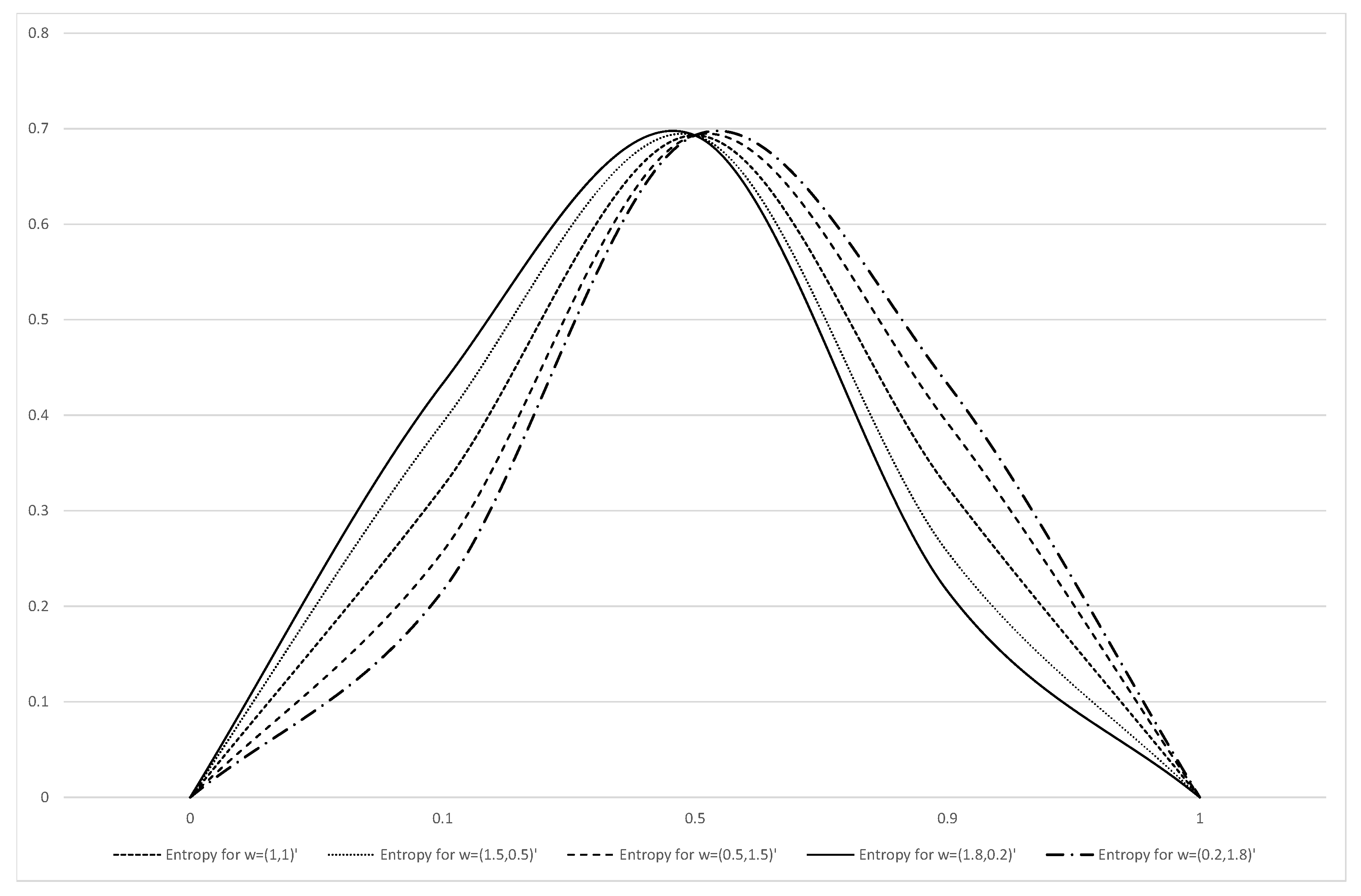
4.1. Weighted Shannon Entropy

Example 3.

Assume a coin toss, the random variable X which enumerates the probability of heads is described by a Bernoulli distribution with probability p. In

Table 1. The Weighted Shannon Entropy for $X\sim B(1,p)$.

	$\mathit{p}=0.1$	$\mathit{p}=0.5$	$\mathit{p}=0.9$
$\underset{\tilde{}}{w}={(1,1)}^T$	0.325	0.693	0.325
$\underset{\tilde{}}{w}={(1.5,0.5)}^T$	0.392	0.693	0.257
$\underset{\tilde{}}{w}={(0.5,1.5)}^T$	0.257	0.693	0.392
$\underset{\tilde{}}{w}={(1.8,0.2)}^T$	0.433	0.693	0.216
$\underset{\tilde{}}{w}={(0.2,1.8)}^T$	0.216	0.693	0.433

we present the weighted entropy of this variable for various p and $\underset{\tilde{}}{w}$.

The above results show that under the equiprobable condition (equal weights) the Shannon Entropy is symmetric around its maximum value but in all other cases with unequal weights (associated with unequal significance) the Weighted Shannon Entropy ends to be symmetric. All these are depicted in Figure 1.

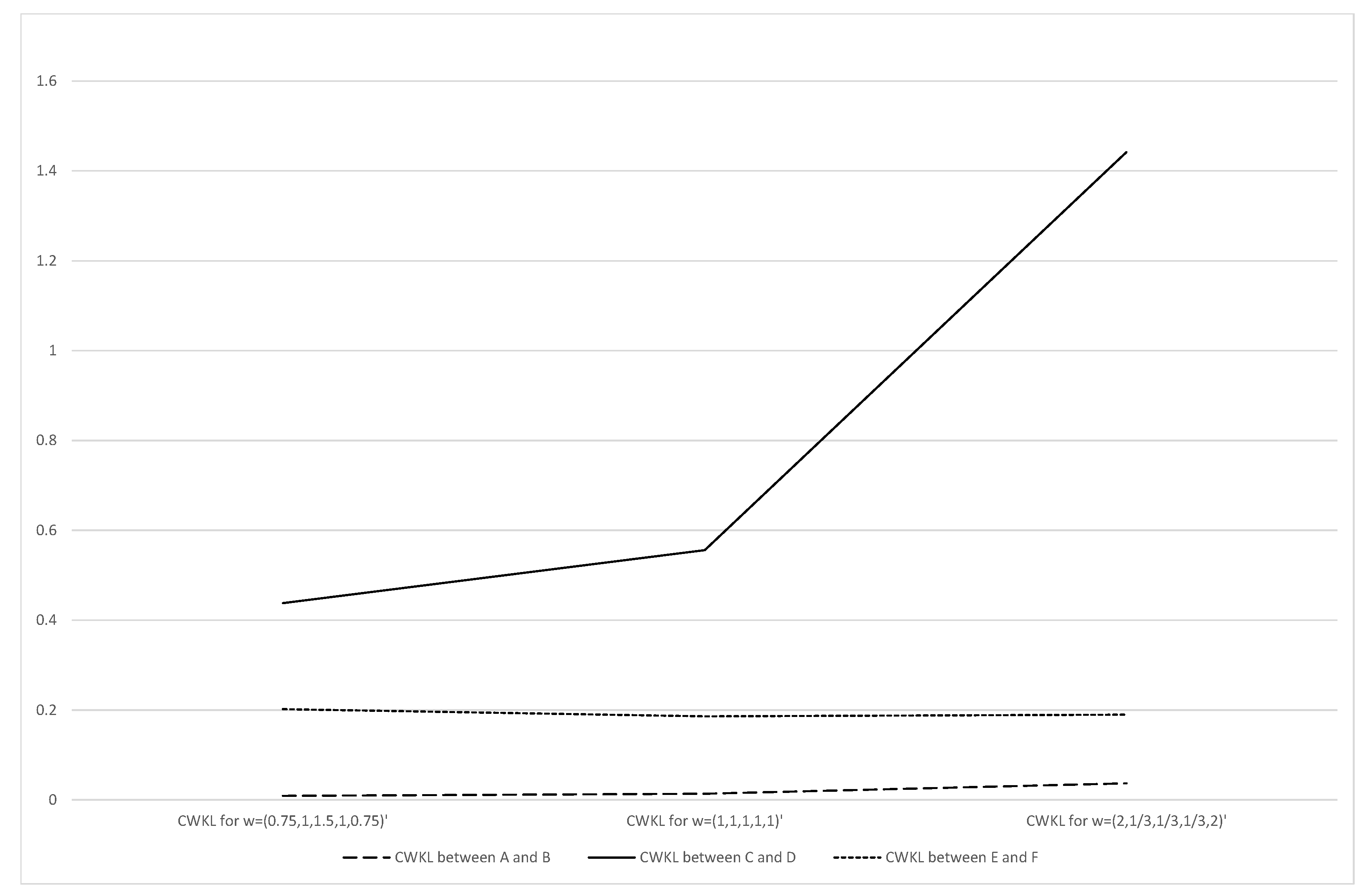
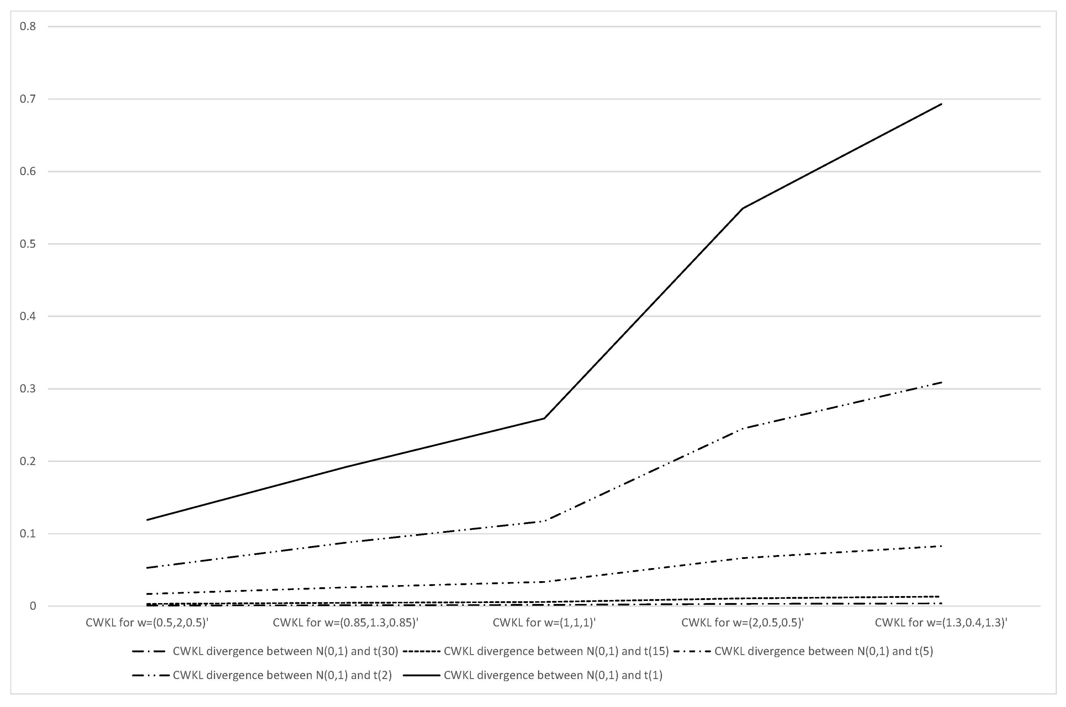
4.2. CWKL Divergence

In this subsection we present examples of the CWKL divergence and consider cases based on several distributions with various weights and our aim is to examine whether small dissimilarities between the two distributions are easily distinguished by the directed measures.

Example 4.

Consider the assets, A, B, C, D, E and F. The returns associated with five states and the probability of each to occur are given in

Table 2. The returns of assets A-F with 5 states and their associated probabilities.

State i	Return	A(${\mathit{p}}_{\mathit{i}}$)	B(${\mathit{q}}_{\mathit{i}}$)	C(${\mathit{p}}_{\mathit{i}}$)	D(${\mathit{q}}_{\mathit{i}}$)	E(${\mathit{p}}_{\mathit{i}}$)	F(${\mathit{p}}_{\mathit{i}}$)
1	$1\%$	$0.1$	$0.14$	$0.05$	$0.3$	$0.1$	$0.05$
2	$3\%$	$0.21$	$0.22$	$0.25$	$0.1$	$0.25$	$0.15$
3	$5\%$	$0.38$	$0.35$	$0.4$	$0.2$	$0.3$	$0.6$
4	$8\%$	$0.21$	$0.22$	$0.25$	$0.1$	$0.25$	$0.15$
5	$10\%$	$0.1$	$0.07$	$0.05$	$0.3$	$0.1$	$0.05$

:

In

Table 3. CWKL divergence between assets A-F for various weights.

	${\mathit{D}}_{\mathit{CKL}}^{\mathit{w}}({\mathit{P}}_{\mathit{A}},{\mathit{Q}}_{\mathit{B}})$	${\mathit{D}}_{\mathit{CKL}}^{\mathit{w}}({\mathit{P}}_{\mathit{C}},{\mathit{Q}}_{\mathit{D}})$	${\mathit{D}}_{\mathit{CKL}}^{\mathit{w}}({\mathit{P}}_{\mathit{E}},{\mathit{Q}}_{\mathit{F}})$
$\underset{\tilde{}}{w}={(1,1,1,1,1)}^T$	$0.013$	$0.556$	$0.186$
$\underset{\tilde{}}{w}={(2,0.333,0.333,0.333,2)}^T$	$0.036$	$1.442$	$0.189$
$\underset{\tilde{}}{w}={(0.75,1,1.5,1,0.75)}^T$	$0.009$	$0.438$	$0.202$

we presented the Corrected Weighted Kullback Leibler (CWKL) divergence between the assets A,B,C,D,E and F for various vectors of weights.

As we can easily see the probability distributions of the assets like A and B are quite similar in contrast with C and D which defers a lot in the ‘extreme’ states (1 and 5) or E and F which have greater dissimilarity in the state 3. From Table 3 we can identify that if we focus on the states with greater dissimilarities then the CWKL divergence increase. All the above are visualized in Figure 2.

Example 5.

Let P be a Standard Normal distribution and Q a Student’s t-distribution with one degree of freedom (df = 1). The CWKL divergence between P and Q for various weights $\underset{\tilde{}}{w}$ applied in different parts of the support is given in

Table 4. CWKL divergence between P and Q in two different partitions of the support.

	${\mathbf{S}}_1=(-\infty ,-3),{\mathbf{S}}_2=(-3,3),{\mathbf{S}}_3=(3,\infty )$	${\mathbf{S}}_1=(-\infty ,-1.85),{\mathbf{S}}_2=(-1.85,1.85),{\mathbf{S}}_3=(1.85,\infty )$
$\underset{\tilde{}}{w}={(1,1,1)}^T$	$0.259$	$0.259$
$\underset{\tilde{}}{w}={(1.3,0.4,1.3)}^T$	$0.693$	$0.738$
$\underset{\tilde{}}{w}={(0.85,1.3,0.85)}^T$	$0.192$	$0.185$
$\underset{\tilde{}}{w}={(2,0.5,0.5)}^T$	$0.549$	$0.579$
$\underset{\tilde{}}{w}={(0.5,2,0.5)}^T$	$0.119$	$0.098$

:

Now, let P be a Standard Normal distribution and Q a Student’s t-distribution with thirty degrees of freedom (df = 30). The CWKL divergence between P and Q for various weights $\underset{\tilde{}}{w}$ applied in different parts of the support is given in

Table 5. CWKL divergence between P and Q in two different partitions of the support.

	${\mathbf{S}}_1=(-\infty ,-3),{\mathbf{S}}_2=(-3,3),{\mathbf{S}}_3=(3,\infty )$	${\mathbf{S}}_1=(-\infty ,-1.85),{\mathbf{S}}_2=(-1.85,1.85),{\mathbf{S}}_3=(1.85,\infty )$
$\underset{\tilde{}}{w}={(1,1,1)}^T$	$0.0016$	$0.0016$
$\underset{\tilde{}}{w}={(1.3,0.4,1.3)}^T$	$0.0037$	$0.0051$
$\underset{\tilde{}}{w}={(0.85,1.3,0.85)}^T$	$0.0013$	$0.0011$
$\underset{\tilde{}}{w}={(2,0.5,0.5)}^T$	$0.0030$	$0.0039$
$\underset{\tilde{}}{w}={(0.5,2,0.5)}^T$	$0.0009$	$0.0004$

:

In Figure 3 we visualize the variations of the CWKL between a Standard Normal distribution and a Student’s t-distribution with various degrees of freedom (df). A plethora of weights are applied on a fixed partition of the support $S_1=(-\infty ,-3),S_2=(-3,3),S_3=(3,\infty )$.

In Example 6 we revisit a real life case proposed by Johnson and Wichern [26] and used by Avlogiaris et al., [13] to study the performance of Local Divergence Measures. The example deals with the grade point average (GPA) scores of 85 students who apply to a business school. Students are categorized in three groups\populations according to their GPA performance as ${\pi }_1$: admit, ${\pi }_2$: do not admit and ${\pi }_3$: borderline. Sample means and variances of each group together with the group sample sizes are given in

Table 6. Sample mean and variance for the three groups of grade point average (GPA) scores.

Population	Sample Size	Estimates
${\pi }_1$	31	${\overline{x}}_1=3.4, s_1^2=0.04$
${\pi }_2$	28	${\overline{x}}_2=2.48, s_2^2=0.03$
${\pi }_3$	26	${\overline{x}}_3=2.99, s_3^2=0.03$

. The aim of Example 6 is to investigate the dissimilarities between the distributions which describe each population and to compare the results with those provided by Avlogiaris et al., [13].

Example 6.

A proper distribution to describe each population, according to Avlogiaris et al., [13] is the Normal distribution with the estimated parameters of each population given in Table 6. So, we have: ${\pi }_1\sim N(3.4,0.04), {\pi }_2\sim N(2.48,0.03)$ and ${\pi }_3\sim N(2.99,0.03)$. In

Table 7. CWKL divergence between ${\pi }_1$ and ${\pi }_2$.

	${\mathbf{S}}_1=(-\infty ,2), {\mathbf{S}}_2=(2,3), {\mathbf{S}}_3=(3,4), {\mathbf{S}}_4=(4,\infty )$
$\underset{\tilde{}}{w}={(1,1,1,1)}^T$	$14.129$
$\underset{\tilde{}}{w}={(0,0,1,0)}^T$	$13.421$
$\underset{\tilde{}}{w}={(0,0,2,1)}^T$	$13.431$
$\underset{\tilde{}}{w}={(0,1,0,0)}^T$	$43.139$
$\underset{\tilde{}}{w}={(1,2,0,0)}^T$	$43.261$

,

Table 8. CWKL divergence between ${\pi }_1$ and ${\pi }_3$.

	${\mathbf{S}}_1=(-\infty ,2.7), {\mathbf{S}}_2=(2.7,3.2), {\mathbf{S}}_3=(3.2,3.7), {\mathbf{S}}_4=(3.7,\infty )$
$\underset{\tilde{}}{w}={(1,1,1,1)}^T$	$2.821$
$\underset{\tilde{}}{w}={(0,0,1,0)}^T$	$2.277$
$\underset{\tilde{}}{w}={(0,0,2,1)}^T$	$2.492$
$\underset{\tilde{}}{w}={(0,1,0,0)}^T$	$3.221$
$\underset{\tilde{}}{w}={(1,2,0,0)}^T$	$3.365$

and

Table 9. CWKL divergence between ${\pi }_2$ and ${\pi }_3$.

	${\mathbf{S}}_1=(-\infty ,2.3), {\mathbf{S}}_2=(2.3,2.8), {\mathbf{S}}_3=(2.8,3.2), {\mathbf{S}}_4=(3.2,\infty )$
$\underset{\tilde{}}{w}={(1,1,1,1)}^T$	$4.331$
$\underset{\tilde{}}{w}={(0,1,0,0)}^T$	$2.925$
$\underset{\tilde{}}{w}={(1,2,0,0)}^T$	$3.341$
$\underset{\tilde{}}{w}={(0,0,1,0)}^T$	$19.981$
$\underset{\tilde{}}{w}={(0,0,2,1)}^T$	$21.726$

we present the CWKL divergence between each pair of populations for appropriate parts of the support.

As we can observe, when we focus on the parts where one of the two distributions is heavier then the CWKL divergence increases. This means that all distributions are far from each other, a result that has also been verified by Avlogiaris et al. [13]. Nevertheless, in our case since, as opposed to the Local Divergence Measures (Avlogiaris et al., [13]), we do not discard the information of the less significant parts, we can easily identify not only whether the distributions differ but also in which parts they differ the most. For that purpose as we give attention to the more ‘extreme’ parts of the distributions (for ${\pi }_1$ and ${\pi }_2$ the $(-\infty ,2)$, for ${\pi }_1$ and ${\pi }_3$ the $(-\infty ,2.7)$ and for ${\pi }_2$ and ${\pi }_3$ the $(3.2,\infty ))$ the divergence increases, which means that they differ considerably as we ‘move’ to the tail of each.

5. Conclusions

The present study succeeds in revealing that the results based on the classical and the weighted entropies and divergences are entirely different and directly related to the specific parts of the distributions we focus on.

The above results show the behaviour of the Weighted Shannon Entropy and clearly show the effect of weights as they applied to specific parts of the distribution. Such results can be used as important probabilistic tools for descriptive as well as discriminatory purposes.

Also, as a conclusion from the above simulations the CWKL divergence is larger (smaller) than the Corrected Kullback–Leibler divergence if we apply bigger weights on the parts with greater (less) dissimilarities. At the same time Corrected Kullback–Leibler divergence is a special case of CWKL divergence when equal weights are applied.

As it is clear from all the above, the appropriate choice of weights will result in better discrimination between similar distributions. In addition, they provide us with a framework for concentrating on the ‘important’ parts of the distribution. Here, we have to mention that the choice of the weights is absolutely subjective and it is related with the belief of the researcher about the significance of each part of the domain. Nevertheless, if someone wishes to identify the parts of the domain of the distributions with the highest dissimilarities an iterative approach could be adopted. Indeed, firstly, the regions of the domain we want to study must be clearly established, then the sum of the weights must be fixed and with multiple iterations (with simultaneous permutations of the weights over the regions) we maximize the CWKL divergence.

These weighted measures could be a useful tool for the construction of ‘directed’ statistical tests on the parts of the distribution we wish to emphasize. Such tests could include goodness of fit tests or model selection criteria which will concentrate on specific parts of the distribution by assigning appropriate weights. Also, the use of weighted divergences could turn out to be useful in financial time series analysis. It is not unusual for a single stochastic model like the Barndorff–Nielsen and Shephard (BN-S) model ([27,28,29]) to fail to describe adequately derivative or commodity market dynamics. For various financial time series data, jumps that often play an important role are typically captured by a Lévy process. The weighted divergences could be incorporated into the analysis of Lévy processes for capturing (identifying) the fluctuations in the jump term of such processes. This way, the jump term could be replaced or modified accordingly, resulting in a more effective and efficient modelling approach. Thus, there is much room for improvement and research on this promising concept.

References

1. Nawrocki, D.N.; Harding, W.H. State-value weighted entropy as a measure of investment risk. Appl. Econ. 1986, 18, 411–419. [Google Scholar] [CrossRef]
2. Basseville, M. Distance measures for signal processing and pattern recognition. Signal Process. 1989, 18, 349–369. [Google Scholar] [CrossRef] [Green Version]
3. Jimenez-Gamero, M.D.; Batsidis, A. Minimum distance estimators for count data based on the probability generating function with applications. Metrika 2017, 80, 503–545. [Google Scholar] [CrossRef]
4. Pardo, L. Statistical Inference Based on Divergence Measures; CRC Press: Boca Raton, FL, USA, 2005. [Google Scholar]
5. Cressie, N.; Read, T.R. Multinomial goodness-of-fit tests. J. R. Stat. Soc. Ser. B Methodol. 1984, 46, 440–464. [Google Scholar] [CrossRef]
6. Lee, S.; Vonta, I.; Karagrigoriou, A. A maximum entropy type test of fit. Comput. Stat. Data Anal. 2011, 55, 2635–2643. [Google Scholar] [CrossRef]
7. Cavanaugh, J.E. Criteria for linear model selection based on Kullback’s symmetric divergence. Aust. N. Z. J. Stat. 2004, 46, 257–274. [Google Scholar] [CrossRef]
8. Shang, J.; Cavanaugh, J.E. Bootstrap variants of the Akaike information criterion for mixed model selection. Comput. Stat. Data Anal. 2008, 52, 2004–2021. [Google Scholar] [CrossRef]
9. Toma, A. Model selection criteria using divergences. Entropy 2014, 16, 2686. [Google Scholar] [CrossRef] [Green Version]
10. Guiaşu, S. Weighted Entropy. Rep. Math. Phys. 1971, 2, 165–179. [Google Scholar] [CrossRef]
11. Frank, O.; Men é ndez, M.L.; Pardo, L. Asymptotic distributions of weighted divergence between discrete distributions. Commun. Stat. Theory Methods 1998, 27, 867–885. [Google Scholar] [CrossRef]
12. Barbu, V.S.; Karagrigoriou, A.; Preda, V. Entropy and divergence rates for markov chains: II. The weighted case. Proc. Rom. Acad. Ser. A 2018, 1, 3–10. [Google Scholar]
13. Avlogiaris, G.; Micheas, A.; Zografos, K. On local divergences between two probability measures. Metrika 2016, 79, 303–333. [Google Scholar] [CrossRef]
14. Belis, M.; Guiaşu, S. A quantitative-qualitative measure of information in cubernetic systems. IEEE Trans. Inf. Theory 1968, 14, 593–594. [Google Scholar] [CrossRef]
15. Guiaşu, S. Grouping data by using the weighted entropy. J. Stat. Plan. Inference 1990, 15, 63–69. [Google Scholar] [CrossRef]
16. Di Crescenzo, A.; Longobardi, M. On weighted residual and past entropies. arXiv 2007, arXiv:math/0703489. [Google Scholar]
17. Suhov, Y.; Zohren, S. Quantum weighted entropy and its properties. arXiv 2014, arXiv:11411.0892. [Google Scholar]
18. Shannon, C.E. A mathematical theory of communication. Bell Syst. Tech. J. 1948, 27, 379–423. [Google Scholar] [CrossRef] [Green Version]
19. Moddemeijer, R. On estimation of entropy and mutual information of continuous distributions. Signal Process. 1989, 16, 233–248. [Google Scholar] [CrossRef] [Green Version]
20. Marsh, C. Introduction to Continuous Entropy; Department of Computer Science, Princeton University: Princeton, NJ, USA, 2013. [Google Scholar]
21. Kullback, S.; Leibler, R. On information and sufficiency. Ann. Math. Stat. 1951, 22, 571–575. [Google Scholar] [CrossRef]
22. Kapur, J.N. Measures of Information and Their Applications; Publishing House: New York, NY, USA, 1994. [Google Scholar]
23. Csiszar, I. On infinite products of random elements and infinite convolutions of probability distributions on locally compact groups. Z. Wahrscheinlichkeitstheorie verw Gebiete 1966, 5, 279–295. [Google Scholar] [CrossRef]
24. Zografos, K.; Ferentinos, K.; Papaioannou, T. Divergence statistics: Sampling properties and multinomial goodness of fit and divergence tests. Commun. Stat. Theory Methods 1990, 19, 1785–1802. [Google Scholar] [CrossRef]
25. Morales, D.; Pardo, L.; Vajda, I. Asymptotic divergence of estimates of discrete distributions. J. Stat. Plan. Inference 1995, 48, 347–369. [Google Scholar] [CrossRef]
26. Johnson, R.A.; Wichern, D.W. Applied Multivariate Statistical Analysis, 3rd ed.; Publishing House, Prentice Hall International Editions: Englewood Cliffs, NJ, USA, 1992. [Google Scholar]
27. Barndorff-Nielsen, O.E.; Shephard, N. Non-Gaussian Ornstein-Uhlenbeck-based models and some of their uses in financial economics. J. R. Stat. Soc. Ser. B 2001, 63, 167–241. [Google Scholar] [CrossRef]
28. Barndorff-Nielsen, O.E.; Shephard, N. Modelling by Lévy processes for financial econometrics. In Lévy Processes; Birkhäuser: Boston, MA, USA, 2001; pp. 283–318. [Google Scholar]
29. Barndorff-Nielsen, O.E. Superposition of Ornstein-Uhlenbeck type processes. Theory Probab. Appl. 2001, 45, 175–194. [Google Scholar] [CrossRef]
Figure 1. Weighted Shannon Entropy of Bernoulli trials.
Mathematics 08 00587 g001
Figure 2. CWKL divergence between assets.
Mathematics 08 00587 g002
Figure 3. CWKL divergence between Standard Normal and various Student’s t-distributions.
Mathematics 08 00587 g003