An Evolve-Then-Correct Reduced Order Model for Hidden Fluid Dynamics

Abstract

In this paper, we put forth an evolve-then-correct reduced order modeling approach that combines intrusive and nonintrusive models to take hidden physical processes into account. Specifically, we split the underlying dynamics into known and unknown components. In the known part, we first utilize an intrusive Galerkin method projected on a set of basis functions obtained by proper orthogonal decomposition. We then present two variants of correction formula based on the assumption that the observed data are a manifestation of all relevant processes. The first method uses a standard least-squares regression with a quadratic approximation and requires solving a rank-deficient linear system, while the second approach employs a recurrent neural network emulator to account for the correction term. We further enhance our approach by using an orthonormality conforming basis interpolation approach on a Grassmannian manifold to address off-design conditions. The proposed framework is illustrated here with the application of two-dimensional co-rotating vortex simulations under modeling uncertainty. The results demonstrate highly accurate predictions underlining the effectiveness of the evolve-then-correct approach toward real-time simulations, where the full process model is not known a priori.

1. Introduction

In the fluid mechanics community, flow systems are often characterized by excessively large spatio-temporal scales. This puts a severe restriction on efficient deployment of practical applications, which usually require near real-time and many-query responses. Traditional full-order simulations cannot achieve this since their computational cost cannot be handled even with the largest supercomputers. Therefore, reduced order modeling emerges as a natural choice to tackle the computationally expensive problems with acceptable accuracy [1,2,3,4,5,6,7,8]. In reduced order models (ROMs), the evolution of the most important and relevant features can be tracked rather than simulating each point in the flow field. These features represent the dynamics of the underlying flow patterns, also called basis functions or modes.

Proper orthogonal decomposition (POD) is a common technique to extract the dominant modes that contribute most to the total system’s energy [9]. POD, coupled with Galerkin projection (GP), has been used for many years to formulate ROMs for dynamical systems [10,11,12,13]. In these ROMs, the full-order set of equations is projected onto the reduced space, resulting in a dynamical system (in modal coefficients) with much lower order than the full order model (FOM). Clearly, this type of ROM is limited to systems for which we have access to the governing equations. That is why they are called intrusive ROMs. However, in many situations, there is a discrepancy between the governing equations and the observed system. This might result from the approximation of underlying phenomena, incorrect parameterization, or insufficient information about source terms embedded within the system. This is, in particular, evident in atmospheric and geophysical systems where many complex phenomena and source terms interact with each other in different ways [14,15,16].

Conversely, pure data-driven techniques, also known as nonintrusive, solely depend on observed data to model the system of interest. Therefore, more complicated processes can be modeled without the need to formulate them with mathematical expressions [17]. Machine learning (ML) tools have shown substantial success in the fluid mechanics community, identifying the underlying structures and mimicking their dynamics [18,19,20,21,22,23,24,25]. However, end-to-end modeling with ML, especially deep learning, has been facing stiff opposition, both in academia and industry, because of the black-box nature and lack of interpretability and generalizability, which might produce nonphysical results [26,27,28]. Even when the input and output data used for training ML algorithms are physically accurate, interpolated quantities by an ML approach can deviate substantially from a physically accurate solution. A perspective on machine learning for advancing fluid mechanics is available in a recent review article [20].

Hybridization of both of the aforementioned approaches is therefore sought to maximize their pros and mitigate their cons [28,29]. Several research efforts have been devoted to achieving this hybridization, for example, in the form of closure modeling [30,31,32,33,34], accelerating simulations [35], controlling numerical oscillations in a higher order numerical solver [36], and enforcing physical laws by tailoring loss functions [37,38,39,40]. In this paper, we address the problem of hidden physics, or unknown source terms, by utilizing a data-driven model with the assumption that the observed data are a manifestation of all interacting mechanisms and sources. The fundamental difference between this study and previous studies is that the automatic pattern-identification capability of learning algorithms is exploited to learn both closure modeling (i.e., the effect of truncated modes in ROM) and the hidden physics (i.e., the unmodeled part in the governing equations) all together. For example, we might have the data observed using RADAR or LiDAR for the underlying transport phenomena. The physical model presenting the vortex merging process might not account for certain parameters such as humidity and temperature on the evolution of vortices. The observed data, on the other hand, comprise these effects, and data-driven methods can be employed to model these effects. We also highlight that our correction formulation implicitly includes the effects of the nonlinear interactions between retained and truncated scales to improve the representation power on reduced dimensions.

If the physical model is incomplete, the GP cannot account for hidden physics embedded within the system. Therefore, we utilize data-driven methods to model this hidden physics information. We first demonstrate the performance of least-squares regression with the quadratic approximation to model the evolution of hidden physics present in the system. Even though this is an interpretable approach, it has limited prediction capability due to its quadratic approximation. In the second framework, a long short-term memory (LSTM) architecture, a variant of recurrent neural networks, is used to account for the unknown physics by learning a correction term representing the discrepancy between the physical model and actual observations. This is the part where intrusive ROM fails. Meanwhile, the generalizability of the model under different operating conditions is retained by employing intrusive (physics-based) ROM to represent the core dynamics. In other words, the underlying physics is divided into two parts, the known part (core physics) modeled by intrusive approaches (e.g., Galerkin ROM) and the unknown part (hidden physics) modeled by nonintrusive approaches (e.g., LSTM). A similar framework was presented in another study where we proposed a modular hybrid analysis and modeling (HAM) approach to account for hidden physics in parameterized systems [41]. The main difference between the two studies is the mechanism of adding a correction to the GP model. In the previous study, the GP model was corrected dynamically with the LSTM model at each time step, and the corrected modal coefficients were used to predict the future state recursively. In the present study, we propose an evolve-then-correct (ETC) approach to account for the hidden physics where the GP and LSTM models are segregated. First, the GP model is used to evolve the initial state to the final time based on the known core dynamics. Then, a correction from the LSTM model is added to the time instant of interest. This means that the GP model evolves with uncorrected modal coefficients, and the correction is enforced statically as a final post-processing step. In other words, in the present study, we learn and enforce a “global” correction, rather than a local one as in [41]. This global correction accounts for the propagation and accumulation of the numerical error from solving GP ROM in addition to the closure effects and hidden physics. This, in turn, provides more insight about the stability performance of the LSTM corrector for long time intervals. Meanwhile, in addition to the LSTM correction, we also study the possibility of imposing a quadratic formula correction following the physics-based GP model.

Relevant to our ETC approach, an evolve-then-filter approach was introduced by Wells et al. [42] as ROM regularization. In their study, GP ROM was evolved for one time step, after which a spatial filter was applied to filter the intermediate solution obtained in the evolve step. This filtering reduces the numerical oscillation of the flow variables (i.e., adds numerical stabilization to ROM). More recently, Gunzburger et al. [43] proposed an evolve-filter-relax approach for uncertainty quantification of the time-dependent Navier–Stokes equations in convection-dominated regimes. This is similar to the evolve-then-filter approach with the additional step of relaxation, which averages the unfiltered and filtered flow variables to control the amount of numerical dissipation introduced by the filter.

In the present paper, we put forth an ETC methodology to take hidden physics into account for superparameterized systems and devise two different data-driven approaches: a least-squares regression-based model and a nonintrusive memory embedding neural network model. An illustration of the proposed framework is provided in solving fluid flow problems governed by the two-dimensional vorticity transport equation. We highlight that our ETC is modular in the sense that it does not require any change in the legacy codes and can be considered as an enabler for parametric model order reduction of partial differential equations. Due to rapid progress in machine learning formulations for ROMs, Section 2 provides a brief overview of the state-of-the-art applications of neural networks in transport processes. We present two variants of the ETC framework in Section 3. The results for numerical experiments with the ETC framework for the vortex-merging process are discussed in Section 4. Finally, Section 5 summarizes our conclusions and highlights some extensions of our approach.

2. Motivating Examples

The POD is one of the most widely used methods to extract the most energetic modes of the system [5,9] and has been used for various fluid flows, ranging from simple, canonical flows to highly complex, real-world engineering applications [7,44]. Barbagallo et al. [45] introduced bi-orthogonal projection for closed-loop control of separated flows and demonstrated its efficient performance against POD for two-dimensional incompressible flow over an open square cavity. In addition to control applications, POD have been used for design optimization of airfoils [46], identification of coherent structures in turbulent flows [47], data assimilation of wind-driven circulation gyre flow [48], variational data assimilation of urban environmental flows [49], and model reduction of thermally buoyant flows [50].

Despite the success of standard POD-GP ROMs, they are limited in their capability to handle complex flows, which are characterized by multiple scales in space and time [31,42,51,52]. In particular, there have been successful efforts to make POD-GP ROM work for the post-transient flow (e.g., nonlinear eddy-viscosities leading to guaranteed boundedness [53,54] or force terms accounting for the neglected high-frequency components). However, challenges arise for strongly transient flows, as well as off-design conditions. Neural networks can be used to obtain robust and stable ROMs for such complex flows. For example, the nonlinear basis functions of a high-dimensional dynamical system can be constructed using a neural network. A neural network can be considered as an extension and generalization of the POD, which provides a more efficient representation of the data [55]. Milano and Koumoutsakos [56] developed a feedforward neural network methodology to reconstruct the near-wall field in turbulent flows and showed the improved prediction capability of the near-wall velocity field with nonlinear neural networks. With the recent advancement in deep learning, nonlinear basis functions can be computed in a computationally efficient manner using convolutional autoencoders (CAE) [57]. Lee and Carlberg [25] proposed a model reduction framework by projecting dynamical systems on nonlinear manifolds using minimum residual formulations. They computed nonlinear manifolds with CAEs and presented the framework for advection-dominated problems exhibiting slowly decaying Kolmogorov n-width. Xu and Duraisamy [58] used CAEs to compute nonlinear manifolds for predictive modeling of spatio-temporal dynamics over a range of parameters. Mohan et al. [59] utilized CAEs for dimensionality reduction of three-dimensional turbulent flows.

The dynamics of the system on the reduced order space is usually modeled using GP, which relies on the governing equations of the system. The GP often suffers from instabilities due to the truncation of lower energy modes and often requires some type of closure to build stable ROMs [60,61,62,63]. Recently, neural networks have become popular for predicting the dynamics of spatio-temporal chaotic systems. Vlachas et al. [64] introduced a data-driven forecasting method for high-dimensional systems by inferring their dynamics in reduced order space with LSTM recurrent neural networks. Pathak et al. [65] developed a hybrid forecasting method that utilizes reservoir computing along with the knowledge-based model and demonstrated its longer prediction performance for the Lorenz system and Kuramoto–Sivashinsky equations. Chen and Xiu [66] presented a generalized residual network framework for learning unknown dynamical systems that learn the discrepancy observation data and the prediction made by another model.

The accurate time series prediction capability of recurrent neural networks has also been exploited to obtain stable and accurate ROMs. For example, Rahman et al. [67] developed a nonintrusive ROM for quasi-geostrophic flows by training LSTM network for modal coefficients extracted from the projection of high-resolution data snapshot on a reduced order basis computed with POD. Ahmed et al. [68] introduced nonintrusive ROM based on LSTM and principal interval decomposition to account for modal deformation for non-ergodic flows. Lui and Wolf [69] developed ROMs for turbulent flows over an airfoil by using spectral POD for dimensionality reduction and a feedforward neural network for the regression of modal coefficients. Zucatti et al. [70] assessed the performance of physics-based and data-driven ROMs for convective heat transfer in a rectangular cavity. They applied the sparse identification of nonlinear dynamics (SINDY) approach and feedforward neural network for modeling the dynamics on the reduced order basis. Wang et al. [71] demonstrated a nonintrusive ROM using POD and an LSTM network for ocean gyre fluid flows. Wu et al. [72] presented a nonintrusive ROM based on POD and a temporal convolutional neural network (CNN) for modeling lower dimensional features. They illustrated the efficiency of temporal CNN in terms of fewer training parameters for flow past a cylinder. Nonintrusive ROMs enabled by neural networks are also applied for aerodynamic applications such as unsteady aerodynamic and aeroelastic analysis using multi-kernel neural networks [73,74]. Baiges et al. [75] developed an ROM based on adaptive finite element meshes in which the neural network was employed for learning a correction between coarse and high-fidelity simulations. Nonintrusive ROMs are also built using machine learning algorithms other than neural networks, such as radial basis function methods to generate dynamics on a reduced space [76] and domain-decomposition nonintrusive ROMs for turbulent flows [77,78].

There is also a growing interest in constructing efficient and robust ROMs with CAEs employed for nonlinear basis computation and recurrent neural network for modeling the dynamics in latent space. For example, Gonzalez and Balajewicz [79] demonstrated the performance of deep convolutional recurrent autoencoders for long-term prediction of incompressible cavity flows. Maulik et al. [80] demonstrated the efficient performance of CAEs in identifying nonlinear latent-space dimensions followed by a recurrent neural network for reduced-space time evolution. They tested the framework for advection-dominated PDEs like the viscous Burgers equation and shallow water equations.

Other than using neural networks to build a fully data-driven nonintrusive ROM, there have been many efforts towards using neural networks to correct and augment GP ROMs in a hybrid fashion. The GP ROM often suffers from instabilities for nonlinear systems due to the modal truncation. In GP ROM, the solution trajectory is assumed to live in a reduced subspace spanned by the first few POD modes. Then, the full order model operators are projected onto this subspace. Due to the inherent system nonlinearity, the truncated modes affect the dynamics of the retained modes. To illustrate this, let us consider a simple example as:

$${\displaystyle \frac{\mathrm{d}u}{\mathrm{d}t}}=u^2.$$

(1)

Assume that our state u can be “fully” described by two modes as $u=a_1{\varphi }_1+a_2{\varphi }_2$, which can be rewritten as:

$$\begin{array}{cc}\hfill {\displaystyle \frac{\mathrm{d}(a_1{\varphi }_1+a_2{\varphi }_2)}{\mathrm{d}t}}& ={(a_1{\varphi }_1+a_2{\varphi }_2)}^2\hfill \end{array}$$

(2)

$$\begin{array}{cc}\hfill & =a_1^2{\varphi }_1^2+a_2^2{\varphi }_2^2+2a_1{a}_2{\varphi }_1{\varphi }_2.\hfill \end{array}$$

(3)

It can be seen that the model’s nonlinearity causes an interaction between the two modes (last term). When ${\varphi }_1$ and ${\varphi }_2$ are independent of time and orthogonal (as is the case for POD), an inner product with ${\varphi }_1$ and ${\varphi }_2$ can be performed to give the following:

$$\begin{array}{cc}\hfill {\displaystyle \frac{\mathrm{d}{a}_1}{\mathrm{d}t}}& ={\varphi }_1^T(a_1^2{\varphi }_1^2+a_2^2{\varphi }_2^2+2a_1{a}_2{\varphi }_1{\varphi }_2),\hfill \end{array}$$

(4)

$$\begin{array}{cc}\hfill {\displaystyle \frac{\mathrm{d}{a}_2}{\mathrm{d}t}}& ={\varphi }_2^T(a_1^2{\varphi }_1^2+a_2^2{\varphi }_2^2+2a_1{a}_2{\varphi }_1{\varphi }_2).\hfill \end{array}$$

(5)

Now, if our reduced order approximation includes only one mode (first mode), then the second equation for $a_2$ is truncated, leaving only the equation for ${\displaystyle \frac{\mathrm{d}{a}_1}{\mathrm{d}t}}$. However, this equation also includes the contribution from the truncated $a_2$. In traditional (flat) GP ROM, the effects of the truncated (second) mode on the dynamics of the retained (first) mode are ignored, giving rise to instabilities and inaccuracies as:

$$\begin{array}{cc}\hfill {\displaystyle \frac{\mathrm{d}{a}_1}{\mathrm{d}t}}& ={\varphi }_1^T\left(a_1^2{\varphi }_1^2\right).\hfill \end{array}$$

(6)

Instead, a map can be approximated between $a_1$ and $a_2$ (known as nonlinear GP ROM). However, such a map between different modal coefficients is not guaranteed to exist (e.g., [81]); thus, nonlinear GP ROM may or may not work. Furthermore, even if this map exists, it is usually not straightforward to approximate analytically or empirically (e.g., [82]). To use the power of neural networks of learning nonlinear maps, Wan et al. [32] used LSTMs to compensate the effect of truncated dynamics on the reduced order model. This is usually called closure modeling (inspired by turbulence modeling). The mathematical model represents a continuous representation of the system, while the numerical solution is our discrete approximation of this representation. Usually, there is a gap between the mathematical model and the numerical approximation due to scale under-resolving and truncation. Closure modeling simply tries to fill this gap. However, there exist many situations where the mathematical model by itself provides an incomplete representation of the physical system. This might be due to the existence of some hidden source terms or dynamical processes that we cannot formulate in a closed form. Similarly, this imperfection in the mathematical model can arise from inaccurate parametrization and/or linearizations. Consequently, the solution of the mathematical model at its best will incur an additional error due to those hidden physics. This is depicted graphically in Figure 1, where the green curve represents the “actual” trajectory of the physical system, while the black one represents our best understanding and formulation of that system where this gray area describes the discrepancy due to hidden physics. Finally, due to numerical approximations and truncation, there is a discrepancy between the mathematical model (black curve) and the numerical solution (red curve). Relating this to our toy example described above, the black curve is what we should recover if we include all the modes (two modes) in our solution, but the red one is what we recover with the ROM with one mode. Many efforts have been made to recover this shaded yellow area with closure modeling [42,43,83,84]. Meanwhile, if our model (i.e., $u^2$) is not sufficient to describe the physical process, then the black curve no longer represents the complete physics (i.e., green curve). Therefore, in the present study, we aim to generalize ROM correction to not only include closure effects, but also to account for the imperfections of mathematical models due to hidden physical processes.

3. Evolve-Then-Correct Approach

In this study, we consider the nonlinear dynamical system parameterized with a parameter $\mu$, which has the form:

$${\mathbf{u}}_t(\mu ,\kappa )=\mathbf{F}(\mathbf{u};\mu )+\mathbf{\Pi }(\mathbf{u};\mu ,\kappa ),$$

(7)

where $\mathbf{u}$ is the state of the system, the subscript t denotes the temporal derivative, $\mathbf{F}$ is the dynamical core of the system governing the known processes parameterized by $\mu$, and $\mathbf{\Pi }$ includes the unknown physics. The unknown physics encompasses deviation between the modeled and observed data resulting from several factors such as empirical parameterizations and imperfect knowledge about the physical processes. The $\kappa$ in our study refers to the control parameter modeling the interaction between the dynamical core of the system and hidden physics.

We use the POD to extract the dominant modes representing the above nonlinear dynamical system. We collect the data snapshots ${\mathbf{u}}_1,{\mathbf{u}}_2,\dots ,{\mathbf{u}}_N$∈${\mathbb{R}}^M$ at different time instances. Here, M is the spatial degree of freedom, which is equal to the total number of grid points, and N is the number of snapshots. In POD, we construct a set of orthonormal basis functions that optimally describes the field variable of the system. We form the rectangular matrix $\mathbf{A}\in {\mathbb{R}}^{M\times N}$ consisting of the the data snapshot ${\mathbf{u}}_n$ as its column. Then, we use singular value decomposition (SVD) to compute the left and right singular vectors of the matrix $\mathbf{A}$. In matrix form, the SVD can be written as:

$$\mathbf{A}=\mathbf{W}\mathbf{\Sigma }{\mathbf{V}}^T=\sum _{k=1}^N{\sigma }_k{\mathbf{w}}_k{\mathbf{v}}_k^T,$$

(8)

where $\mathbf{W}\in {\mathbb{R}}^{M\times N}$, $\mathbf{\Sigma }\in {\mathbb{R}}^{N\times N}$, and $\mathbf{V}\in {\mathbb{R}}^{N\times N}$. $\mathbf{W}$ and $\mathbf{V}$ contain the left and right singular vectors, which are identical to the eigenvectors of $\mathbf{A}{\mathbf{A}}^T$ and ${\mathbf{A}}^T\mathbf{A}$, respectively. Furthermore, the square of singular vales is equal to the eigenvalues, i.e., ${\lambda }_k={\sigma }_k^2$. The vectors ${\mathbf{w}}_k$ (also the eigenvectors of $\mathbf{A}{\mathbf{A}}^T$) are the POD basis functions, and we denote them as ${\varphi }_k$ in this text. The POD basis functions are orthonormal (i.e., $\langle {\varphi }_i,{\varphi }_j\rangle ={\delta }_{ij}$) and are computed in an optimal manner in the $L_2$ sense [85,86]. The state of the dynamical system can be approximated using these POD basis functions as follows,

$$\mathbf{u}(\mathbf{x},t)=\sum _{k=1}^R{a}_k\left(t\right){\varphi }_k\left(\mathbf{x}\right),$$

(9)

where R is the number of retained basis functions such that $R<<N$ and $a_k$ are the time-dependent modal coefficients. We note that mean-subtracted (or anomaly) fields are often used in basis construction and building ROMs. However, we opted to use whole field data (i.e., without centering) for the clarity, simplicity, and brevity of the ETC presentation. The POD basis functions minimize the mean squared error between the field variable and its truncated representation. Moreover, it also minimizes the number of basis functions required to describe the field variable for a given error [87]. The number of retained modes is usually decided based on their energy content. Using these retained modes, we can form the POD basis set $\mathsf{\Phi }={\left\{{\varphi }_k\right\}}_{k=1}^R$ to build the ROM.

POD is often complemented with GP to reduce the higher dimensional partial differential equations (PDEs) into reduced order ordinary differential equations (ODEs). To get GP equations, first, we use a linear superposition of the approximated field variable given by Equation (9) into the governing equation of the physical system. Then, we apply the inner product of the resulting equation with the orthonormal basis function ${\varphi }_k$. Therefore, we need the complete information about the governing equation of the physical system to form the GP equations that can describe the system accurately. However, we do not know about the hidden physics given by the source term $\mathbf{\Pi }$ in Equation (7). Therefore, we cannot derive a fully intrusive GP model for such a dynamical system.

In this study, we use two data-driven algorithms to model the hidden physics (i.e., the source term), and GP equations are derived based on the dynamical core of the system $\mathbf{F}$. The GP equations for the system with linear and nonlinear operators can be written as:

$$\dot{\mathbf{a}}=\mathfrak{L}\mathbf{a}+{\mathbf{a}}^T\mathfrak{N}\mathbf{a},$$

(10)

or more explicitly,

$${\displaystyle \frac{\mathrm{d}{a}_k}{\mathrm{d}t}}=\sum _{i=1}^R{\mathfrak{L}}_k^i{a}_i+\sum _{i=1}^R\sum _{j=1}^R{\mathfrak{N}}_k^{ij}{a}_i{a}_j,$$

(11)

where $\mathfrak{L}$ and $\mathfrak{N}$ are the linear and nonlinear operators of the physical system. We limited our formulation in considering quadratic nonlinearity without loss of generality by using R modes. We used the third-order Adams–Bashforth method (AB3) to integrate Equation (11) numerically. In the discrete sense, the update formula can be written as:

$$a_k^{(n+1)}=a_k^{\left(n\right)}+\Delta t\sum _{q=0}^s{\beta }_{q}G\left(a_k^{(n-q)}\right),$$

(12)

where s and ${\beta }_q$ are the constants corresponding to the AB3 scheme, which are $s=2,{\beta }_0=23/12,{\beta }_1=-16/12,$ and ${\beta }_2=5/12$. We can obtain the true projection modal coefficients by simply projecting the field variable onto the basis functions, which can be written as:

$${\alpha }_k^{\left(n\right)}=\langle \mathbf{u}(\mathbf{x},t_n),{\varphi }_k\rangle ,$$

(13)

where the angle parentheses refer to the Euclidean inner product defined as $\langle \mathbf{x},\mathbf{y}\rangle ={\mathbf{x}}^T\mathbf{y}={\sum }_{i=1}^M{x}_i{y}_i$. The true projection modal coefficients include the hidden physics and its interaction with the dynamical core of the system. Note that the GP modal coefficients to be calculated by solving Equation (11) do not model this effect. We can then define the correction term as:

$$\mathrm{Correction}:=C_k^{\left(n\right)}={\alpha }_k^{\left(n\right)}-a_k^{\left(n\right)}.$$

(14)

Our goal in this work is to develop supervised learning frameworks to model the correction term C. Albeit sharing some similarities with other data-driven ROMs with regard to its estimation procedure from available snapshot data, the proposed framework is an attempt to bring correction into our consideration after the model has evolved in time. Therefore, the correction procedure is segregated from the dynamic model updates. This allows us to evolve our process with a physics-based model that captures the essential dynamics and correct our quantity of interest using a supervised correction approach at any desired time. In a nutshell, our approach can be framed as:

$$\begin{array}{|c|}\hline \mathrm{ETC}\mathrm{ROM}=\mathrm{GP}\mathrm{ROM}+\mathrm{Correction}\\ \hline\end{array}$$

or more specifically, at any time, it reads as,

$${\tilde{a}}_k^{\left(n\right)}\leftarrow a_k^{\left(n\right)}+C_k^{\left(n\right)}\left(a_k^{\left(n\right)}\right),$$

(15)

where the superscript tilde refers to the rectified coefficients, and we devise two approaches for estimating the mapping function $C_k^{\left(n\right)}\left(a_k^{\left(n\right)}\right)$ to correct our model update. Furthermore, in certain situations, one might not have a mechanistic model with which to start. This way, we also highlight that our approach can be reduced to a fully nonintrusive method where we can only use the part provided by the supervised learning.

3.1. ETC-LS: Least-Squares Correction

In order to implement the ETC approach, we follow regression techniques to learn a mapping between the GP model predictions ($a_k^{\left(n\right)}$) and the correction given in Equation (14). Different data mining [88,89,90] and symbolic regression [91,92,93,94,95] ideas might be utilized in order to design a model to fit. Inspired by the GP model in Equation (11), we adopt a similar quadratic formula to represent the missing physics as follows:

$${\widehat{\mathfrak{B}}}_k+\sum _{i=1}^R{\widehat{\mathfrak{L}}}_k^i{a}_i^{\left(n\right)}+\sum _{i=1}^R\sum _{j=1}^R{\widehat{\mathfrak{N}}}_k^{ij}{a}_i^{\left(n\right)}{a}_j^{\left(n\right)}={\alpha }_k^{\left(n\right)}-a_k^{\left(n\right)}.$$

(16)

It turns out that Equation (16) has a number of $\mathfrak{D}$ coefficients ($\widehat{\mathfrak{B}}$, $\widehat{\mathfrak{L}}$, and $\widehat{\mathfrak{N}}$) to predetermine, where $\mathfrak{D}\approx R+R^2+R^3$. Indeed, due to the symmetry of $\widehat{\mathfrak{N}}$, the number of unknown coefficients is actually less than that value (i.e., $\mathfrak{D}=R+R^2+R^2(R+1)/2$). In order to evaluate these coefficients, we use training data where ${\alpha }_k^{\left(n\right)}$ and $a_k^{\left(n\right)}$ are known. For every snapshot, we can evaluate Equation (16) as below:

$$\begin{array}{cc}\hfill & {\widehat{\mathfrak{B}}}_1+\sum _{i=1}^R{\widehat{\mathfrak{L}}}_1^i{a}_i^{\left(n\right)}+\sum _{i=1}^R\sum _{j=1}^R{\widehat{\mathfrak{N}}}_1^{ij}{a}_i^{\left(n\right)}{a}_j^{\left(n\right)}={\alpha }_1^{\left(n\right)}-a_1^{\left(n\right)}\hfill \\ \hfill & {\widehat{\mathfrak{B}}}_2+\sum _{i=1}^R{\widehat{\mathfrak{L}}}_2^i{a}_i^{\left(n\right)}+\sum _{i=1}^R\sum _{j=1}^R{\widehat{\mathfrak{N}}}_2^{ij}{a}_i^{\left(n\right)}{a}_j^{\left(n\right)}={\alpha }_2^{\left(n\right)}-a_2^{\left(n\right)}\hfill \\ \hfill & ⋮\hfill \\ \hfill & {\widehat{\mathfrak{B}}}_R+\sum _{i=1}^R{\widehat{\mathfrak{L}}}_R^i{a}_i^{\left(n\right)}+\sum _{i=1}^R\sum _{j=1}^R{\widehat{\mathfrak{N}}}_R^{ij}{a}_i^{\left(n\right)}{a}_j^{\left(n\right)}={\alpha }_R^{\left(n\right)}-a_R^{\left(n\right)},\hfill \end{array}$$

so we have ($N·R$) equations for each value of the control parameter $\mu$ (i.e., totaling a number $\mathfrak{C}=N·R·P$ of equations, where P is the number of parameter values). Note that Equation (16) can be rewritten as a linear system of equations in the standard form of $\widehat{\mathbf{A}}\widehat{\mathbf{z}}=\widehat{\mathbf{b}}$, where $\widehat{\mathbf{A}}\in {\mathcal{R}}^{\mathfrak{C}\times \mathfrak{D}}$, $\widehat{\mathbf{z}}\in {\mathcal{R}}^{\mathfrak{D}}$, and $\widehat{\mathbf{b}}\in {\mathcal{R}}^{\mathfrak{C}}$, where $\widehat{\mathbf{z}}$ represents $\widehat{\mathfrak{B}}$, $\widehat{\mathfrak{L}}$, and $\widehat{\mathfrak{N}}$. Normally, we would usually have a larger number of equations than unknowns (i.e., overdetermined system). Therefore, we can adopt a least-squares (LS) regression approach where the norm of the residual vector ($\parallel \widehat{\mathbf{b}}-\widehat{\mathbf{A}}\widehat{\mathbf{z}}\parallel$) is minimized. As detailed in [33], the solution of this LS problem can be obtained as:

$${\widehat{\mathbf{z}}}_{\mathrm{LS}}=\widehat{\mathbf{V}}{\widehat{\mathbf{\Sigma }}}^{-1}{\widehat{\mathbf{U}}}^T\widehat{\mathbf{b}},$$

(17)

where $\widehat{\mathbf{A}}=\widehat{\mathbf{U}}\widehat{\mathbf{\Sigma }}{\widehat{\mathbf{V}}}^T$ (i.e., the SVD of the matrix $\widehat{\mathbf{A}}$). Herein, the sorted diagonal matrix $\widehat{\mathbf{\Sigma }}=\mathrm{diag}[{\widehat{\sigma }}_1,{\widehat{\sigma }}_2,\dots ,{\widehat{\sigma }}_m,\dots ,{\widehat{\sigma }}_{\mathfrak{D}}]$ can be inverted using a truncated SVD approach since Equation (16) constitutes an ill-posed (rank-deficient) linear system. The truncated SVD inversion hence reads as ${\widehat{\mathbf{\Sigma }}}^{-1}=\mathrm{diag}[1/{\widehat{\sigma }}_1,1/{\widehat{\sigma }}_2,\dots ,1/{\widehat{\sigma }}_m,0,\dots ,0]$, where ${\widehat{\sigma }}_m$ can be determined by a user-specified tolerance (i.e., we retain the singular values of ${\widehat{\sigma }}_k$ that satisfy ${\widehat{\sigma }}_k^2/{\widehat{\sigma }}_1^2>{10}^{-5}$, where $k=1,2,\dots ,m$, and truncate the remaining ones in our computations). After the linear LS problem is solved, the vector $\widehat{\mathfrak{B}}$, matrix $\widehat{\mathfrak{L}}$, and tensor $\widehat{\mathfrak{B}}$ can be constructed, and Equation (16) can be used to estimate the required correction to account for the hidden source terms and closures. Finally, the first correction approach (called ETC-LS in this study) reads as:

$${\tilde{a}}_k^{\left(n\right)}=a_k^{\left(n\right)}+{\widehat{\mathfrak{B}}}_k+\sum _{i=1}^R{\widehat{\mathfrak{L}}}_k^i{a}_i^{\left(n\right)}+\sum _{i=1}^R\sum _{j=1}^R{\widehat{\mathfrak{N}}}_k^{ij}{a}_i^{\left(n\right)}{a}_j^{\left(n\right)},$$

(18)

where we emphasize that the correction can be applied at any desired time since data-driven correction will not affect the evolution trajectory of Galerkin ROM. At the same time, our dynamical model is not fully a black-box since we evolve the process in time using a physics-based model (to our best available knowledge about its behavior) and correct its predictive performance locally in time from archival data.

3.2. ETC-LSTM: Long Short-Term Memory Correction

Although our least-squares treatment in the previous discussion promotes the interpretability of the correction model following the physics-based GP core model, our approximation is limited to the adopted quadratic formula. Now, we can extend this mapping approximation by learning the correction term with one of the state-of-the-art machine learning tools often used in speech recognition and natural language processing. We employ the LSTM architecture [96], a variant of the recurrent neural network, to learn this correction. LSTM networks are particularly suitable for time-series prediction, since they can use the information about the previous state of the system to predict the next state of the system. Therefore, the LSTM architecture has been employed for many nonintrusive ROMs [32,67,68,97] due to its capability of built-in memory-embedding. We trained our LSTM neural network to learn the mapping from GP modal coefficients to the correction term, i.e., $\{a_1,\dots ,a_R\}\in {\mathbb{R}}^R\to \{C_1,\dots ,C_R\}\in {\mathbb{R}}^R$, where $C_k$ is the correction given by Equation (14). We used three lookbacks to be consistent with the AB3 scheme during training (please see the details in [67]). Since GP modal coefficients were used as input features to the LSTM network, the parameter $\mu$ governing the system’s behavior was taken implicitly into account. Once the model was trained, we could correct the GP modal coefficients with LSTM-based correction to approximate true projection modal coefficients. Hence, the second approach can be summarized as:

$${\tilde{a}}_k^{\left(n\right)}=a_k^{\left(n\right)}+C_k^{\left(n\right)},$$

(19)

which we denote as ETC-LSTM when we present our results.

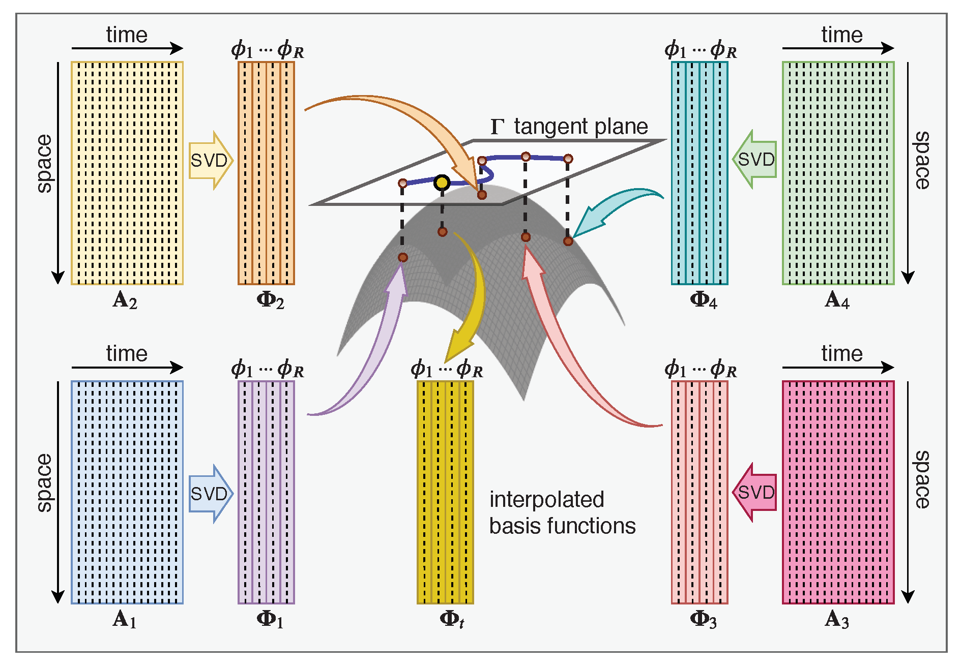
3.3. Grassmann Manifold Interpolation

The ROM requires the basis functions that were obtained using POD on the dataset. The dataset for the POD was generated using FOM and/or collecting snapshots from experimental measurements. Running FOM for every ROM is opposite the motivation behind using ROM. Hence, we should be able to approximate the POD basis functions for the test parameter from existing POD basis sets (included in the training), and we employed Grassmann manifold interpolation [98,99] to achieve this. The training data were generated for different values of parameters ${\mu }_1,\dots ,{\mu }_P$. We computed the separate basis set ${\mathsf{\Phi }}_1,\dots ,{\mathsf{\Phi }}_P$ for each of these parameters. The graphical illustration of the Grassmann manifold interpolation is provided in Figure 2, and the procedure is described in Algorithm 1. We note that the Grassmann manifold interpolation provides substantial speed-ups and computational savings since FOM snapshots need not be collected for every new parameter value. However, the reduced operators $\mathfrak{L}$ and $\mathfrak{N}$ have to be re-computed before the GP ROM can be solved. This might induce a computational overhead compared to GP ROMs with global basis functions, where a unique basis and model operators are used across a wide range of parameters. Meanwhile, this overhead can be reduced by utilizing hyper-reduction techniques tailored to reduce the online computational cost of such operators during the online phase [100,101], like the empirical interpolation method (EIM) [102] or its discrete version, the discrete empirical interpolation method (DEIM) [103,104], gappy POD [105,106], and missing point estimation (MPE) [107,108].

Algorithm 1 Grassmann manifold interpolation.
1:	Given a set of basis functions ${\mathsf{\Phi }}_1,{\mathsf{\Phi }}_2,\dots ,{\mathsf{\Phi }}_P$ corresponding to the offline simulations (i.e., with mapping $S_1,S_2,\dots ,S_P$) parameterized by ${\mu }_1,{\mu }_2,\dots ,{\mu }_P$.
2:	Select a point $S_0\leftarrow S_i\in [S_1,\dots ,S_P]$ corresponding to the basis function set ${\mathsf{\Phi }}_0\leftarrow {\mathsf{\Phi }}_i\in [{\mathsf{\Phi }}_1,\dots ,{\mathsf{\Phi }}_P]$ as the reference point.
3:	Map each point $S_i$ to a matrix ${\mathbf{\Gamma }}_i$, which represents the tangent space using logarithm map ${\mathrm{Log}}_{S_0}$: $$({\mathsf{\Phi }}_i-{\mathsf{\Phi }}_0{\mathsf{\Phi }}_0^T{\mathsf{\Phi }}_i){\left({\mathsf{\Phi }}_0^T{\mathsf{\Phi }}_i\right)}^{-1}={\mathbf{U}}_i{\mathbf{\Sigma }}_i{\mathbf{V}}_i^T,$$ (20) $${\mathbf{\Gamma }}_i={\mathbf{U}}_i{\tan }^{-1}\left({\mathbf{\Sigma }}_i\right){\mathbf{V}}_i^T.$$ (21)
4:	Construct matrix ${\mathbf{\Gamma }}_t$ corresponding to the test parameter ${\mu }_t$ using the Lagrange interpolation of matrices ${\mathbf{\Gamma }}_i$, corresponding to ${\mu }_1,\dots ,{\mu }_P$: $${\mathbf{\Gamma }}_t=\sum _{i=1}^P\left(\prod _{\begin{array}{c}j=1j\ne i\end{array}}^P\frac{{\mu }_t-{\mu }_j}{{\mu }_i-{\mu }_j}\right){\mathbf{\Gamma }}_i.$$ (22)
5:	Compute the POD basis functions ${\mathsf{\Phi }}_{\mathbf{t}}$ corresponding to the test parameter ${\mu }_t$ using the exponential map. $${\mathbf{\Gamma }}_t={\mathbf{U}}_t{\mathbf{\Sigma }}_t{\mathbf{V}}_t^T,$$ (23) $${\mathsf{\Phi }}_t=[{\mathsf{\Phi }}_0{\mathbf{V}}_t\cos \left({\mathbf{\Sigma }}_t\right)+{\mathbf{U}}_t\sin \left({\mathbf{\Sigma }}_t\right)]{\mathbf{V}}_t^T,$$ (24)
	where the trigonometric operators apply only to the diagonal elements.

4. Numerical Results

We demonstrate the performance of ETC framework discussed in Section 3 for the two-dimensional vorticity transport equation. The vorticity transport equation can be written as:

$$\begin{array}{cc}\hfill {\displaystyle \frac{\partial \omega }{\partial t}}+{\displaystyle \frac{\partial \psi }{\partial y}}{\displaystyle \frac{\partial \omega }{\partial x}}-{\displaystyle \frac{\partial \psi }{\partial x}}{\displaystyle \frac{\partial \omega }{\partial y}}& ={\displaystyle \frac{1}{\mathrm{Re}}}\left({\displaystyle \frac{{\partial }^2\omega }{\partial x^2}}+{\displaystyle \frac{{\partial }^2\omega }{\partial y^2}}\right)+\Pi ,\hfill \end{array}$$

(25)

$$\begin{array}{c}\hfill {\displaystyle \frac{{\partial }^2\psi }{\partial x^2}}+{\displaystyle \frac{{\partial }^2\psi }{\partial y^2}}=-\omega ,\end{array}$$

(26)

where $\omega$ is the vorticity defined as $\omega =\nabla \times \mathbf{u}$, $\mathbf{u}={[u,v]}^T$ is the velocity vector, and $\psi$ is the streamfunction. We used vortex merger as the test example. In this test example, a pair of co-rotating vortices that are separated from each other by some distance induces the fluid motion. The vortex merging process has been extensively studied in the two-dimensional context as it explains the average inverse energy and direct enstrophy cascades observed in two-dimensional turbulence [109]. The initial condition for the vortex merger test case is given as:

$$\begin{array}{c}\hfill \omega (x,y,0)=exp\left(-\pi \left[{(x-x_1)}^2+{(y-y_1)}^2\right]\right)+exp\left\{\left(-\pi \left[{(x-x_2)}^2+{(y-y_2)}^2\right]\right)\right\},\end{array}$$

(27)

where their centers are initially located at $(x_1,y_1)=(3\pi /4,\pi )$ and $(x_2,y_2)=(5\pi /4,\pi )$. Figure 3 shows how two co-rotating vortices separated by a certain distance evolve over time in the absence of any source term. We utilized an arbitrary array of Taylor–Green vortices as the source term, which represents a perturbation field (i.e., referring to hidden physics). The source term in Equation (25) is given below:

$$\Pi =-F\left(t\right)\cos \left(\eta x\right)\cos \left(\eta y\right),$$

(28)

where $F\left(t\right)=\gamma e^{-t/\mathrm{Re}}$ and $\eta =3$. The parameter $\gamma$ controls the strength of Taylor–Green vortices. We used computational domain $(x,y)\in [0,2\pi ]$ with periodic boundary conditions. We generated data snapshots for $\mathrm{Re}=[200,400,600,800]$ with a ${256}^2$ spatial grid and a time-step of $0.01$ from time $t=0$ to $t=20$. We tested the ETC framework for the out-of-sample condition at $\mathrm{Re}=1000$. The linear and nonlinear operators in GP equations for two-dimensional vorticity transport equation are:

$$\begin{array}{cc}\hfill {\mathfrak{L}}_k^i& =〈{\displaystyle \frac{1}{\mathrm{Re}}}\left({\displaystyle \frac{{\partial }^2{\varphi }_i^{\omega }}{\partial x^2}}+{\displaystyle \frac{{\partial }^2{\varphi }_i^{\omega }}{\partial y^2}}\right),{\varphi }_k^{\omega }〉,\hfill \end{array}$$

(29)

$$\begin{array}{cc}\hfill {\mathfrak{N}}_k^{ij}& =〈-\left({\displaystyle \frac{\partial {\varphi }_i^{\omega }}{\partial x}}{\displaystyle \frac{\partial {\varphi }_j^{\psi }}{\partial y}}-{\displaystyle \frac{\partial {\varphi }_i^{\omega }}{\partial y}}{\displaystyle \frac{\partial {\varphi }_j^{\psi }}{\partial x}}\right),{\varphi }_k^{\omega }〉,\hfill \end{array}$$

(30)

where ${\varphi }_k^{\omega }$ and ${\varphi }_k^{\psi }$ refer to POD basis functions of the vorticity and streamfunction fields, respectively [110]. We can compute the energy retained by POD basis functions using a relative information content (RIC) formula as given below:

$$\mathrm{RIC}\left(R\right)=\left(\frac{{\sum }_{j=1}^R{\sigma }_j^2}{{\sum }_{j=1}^N{\sigma }_j^2}\right).$$

(31)

In other words, RIC represents the fraction of information (variance) of the the total data that can be recovered using R basis functions. Figure 4 displays the convergence of relative information content with respect to the number of POD basis functions used to represent the reduced order system for different Reynolds number of flow included in the training. We retained eight basis functions (i.e., $R=8$) as they captured more than $99.95\%$ of the energy for all Reynolds numbers included in our training.

We illustrate the ETC approach for two different magnitudes of the source term, $\gamma =0.01$ and $\gamma =0.1$. We used $\mathrm{Re}=800$ as the reference Reynolds number to obtain basis functions using the Grassmann manifold interpolation procedure for both test cases. Figure 5 shows the true basis functions and interpolated basis functions at $\mathrm{Re}=1000$. The Grassmann manifold interpolation procedure can compute correct basis functions with very little deviation (especially for bases ${\varphi }_7$ and ${\varphi }_8$) from true basis functions. We trained the LSTM network with two hidden layers and 80 cells. Our experiments with different hyperparameters showed that the results were not highly sensitive to the choice of hyperparameters.

Figure 6 shows the evolution of vorticity modal coefficients for $\gamma =0.01$. The GP modal coefficients were different from the true projection modal coefficients even though the eight modes were capturing more than $99.95\%$ of the energy. This difference was due to the source term not modeled by GP equations. In the ETC approach, we corrected the GP modal coefficients and obtained excellent agreement with the true modal coefficients after correction. The accuracy of the results obtained with the ETC approach would depend on the approximation capability of the data-driven method used to model the hidden physics. We can see that the ETC-LS framework with its quadratic approximation was able to model the hidden physics correctly. The vorticity modal coefficients obtained with the ETC-LSTM framework were almost the same as the true projection modal coefficients. Figure 7 displays the evolution of the error between true modal coefficients and modal coefficients computed using the GP, ETC-LS, and ETC-LSTM framework.

To show the difference between vorticity modal coefficients for all training and testing Reynolds numbers, we plot the time series of modal coefficients for all Reynolds numbers in the same plot as reported in Figure 8. We can observe that the evolution of vorticity modal coefficients for the test Reynolds number was significantly different from the projection trajectories of each training Reynolds number, and the ETC-LSTM framework was able to produce the correct trajectory of modal coefficients for the test Reynolds number. This also showed that the LSTM had not simply memorized the correction from the training set, but it learned the dependence of modal coefficients on the parameter (through input features) governing the physical system. Since the GP was used to model the core physics of the system, the generalizability was further enforced in the ETC approach.

Figure 9 displays the evolution of modal coefficients for $\gamma =0.1$. We see that there was a large deviation between GP modal coefficients and true projection modal coefficients due to the large magnitude of the source term. The ETC-LS framework was able to correct the trajectory of vorticity modal coefficients especially for the first three modes. However, the ETC-LS framework was limited by quadratic approximation and was inadequate in correcting the trajectory for later modes. Therefore, even though the ETC-LS framework was attractive due to its interpretability, it was limited in its representational capability. The ETC-LSTM framework on the other hand could correct GP modal coefficients and produce the modal coefficients’ trajectories close to the true projection. Figure 10 shows the evolution of error between true modal coefficients and modal coefficients predicted by the GP, ETC-LS, and ETC-LSTM framework for $\gamma =0.1$. Since the source term was very large and had a similar magnitude as the main field, we did not get the same level of accuracy as the test case with $\gamma =0.01$, especially near the end time (i.e., $t=15-20$). Figure 11 presents the vorticity modal coefficients at all training Reynolds numbers and the test Reynolds number.

Finally, Figure 12 shows the three-dimensional plot of the reconstructed vorticity field computed with true projection, GP, ETC-LS, and ETC-LSTM modal coefficients. We did not see a significant difference between the three-dimensional vorticity field computed with GP and ETC modal coefficients for $\gamma =0.01$. However, the orientation of two vortices was not correctly captured by GP modal coefficients in comparison to the true projection. The ETC-LS and ETC-LSTM frameworks correctly predicted the orientation of two vortices close to the true projection. Moreover, there was a large difference between the reconstructed vorticity field for GP and true projection at $\gamma =0.1$. The magnitude of the reconstructed vorticity field with GP modal coefficients was very small compared to the true projection modal coefficients, and it was not able to represent the vorticity field affected by the Taylor–Green vortices. The ETC-LS and ETC-LSTM frameworks correctly predicted the vorticity field with sufficient accuracy and also produced the vorticity field due to the Taylor–Green vortices. The correct prediction of the vorticity field for the large source term illustrated the advantage of the ETC approach for physical systems where there is a large discrepancy between the modeled and observed data due to modeling assumptions, imperfect parameterizations, and insufficient knowledge about the physical system.

We would like to reiterate here that in our study, we assumed that any information about the source term was not available, and hence, we had to employ data-driven methods to model this unknown information. However, if the information about the source term were available, we could include it in the GP model to build accurate ROMs. For a fair comparison, we present the results for ROM with the source term included in the GP model, and we refer to this as the GP (C) model. If we project the source term $\Pi$ given in Equation (28), we get a correction term given by:

$${\mathfrak{b}}_k=\langle \Pi ,{\varphi }_k^{\omega }\rangle ,$$

(32)

and the evolution of the corrected GP (C) model is given by:

$${\displaystyle \frac{\mathrm{d}{a}_k}{\mathrm{d}t}}={\mathfrak{b}}_k+\sum _{i=1}^R{\mathfrak{L}}_k^i{a}_i+\sum _{i=1}^R\sum _{j=1}^R{\mathfrak{N}}_k^{ij}{a}_i{a}_j.$$

(33)

Figure 13 shows the three-dimensional plot of the vorticity field at final time $t=20$ computed with the GP (C) model for $\gamma =0.01$ and $\gamma =0.1$. If we compare Figure 12 and Figure 13, we see an excellent agreement between the true projection vorticity field and the vorticity field computed using the GP (C) model. Therefore, if the physical model used to represent a physical process was accurate and included all the information, then we could recover accurate results with the GP model. However, the main idea in this study was to recover accurate dynamics for physical systems where the interpretable mathematical model did not contain all the information about physical processes, such as the unknown source term, and how to utilize observations in the form of snapshots to correct the incomplete physical model.

To quantify the performance of different frameworks, we defined the root mean squared error (RMSE) between the FOM vorticity field and the vorticity field computed with different ROM frameworks. The RMSE is defined as:

$$\mathrm{RMSE}\left(t_n\right)=\sqrt{\frac{1}{n_x{n}_y}\sum _{i=1}^{n_x}\sum _{j=1}^{n_y}{\left({\omega }^{\mathrm{FOM}}(x_i,y_j,t_n)-{\omega }^{\mathrm{ROM}}(x_i,y_j,t_n)\right)}^2},$$

(34)

where ${\omega }^{\mathrm{FOM}}$ is the FOM vorticity field, ${\omega }^{\mathrm{ROM}}$ is the vorticity field computed using ROM, and $n_x$ and $n_y$ are the number of grid points in both directions.

Table 1. Root mean squared error (RMSE) between the FOM vorticity field and the vorticity field predicted with the true, GP, GP (C), ETC-LS, and ETC-LSTM framework at time $t=20$ with $R=8$ basis functions.

	True	GP	GP (C)	ETC-LS	ETC-LSTM
$\gamma =0.01$	$3.09\times {10}^{-5}$	$1.04\times {10}^{-4}$	$3.25\times {10}^{-5}$	$3.11\times {10}^{-5}$	$3.14\times {10}^{-5}$
$\gamma =0.1$	$8.36\times {10}^{-5}$	$2.21\times {10}^{-3}$	$1.01\times {10}^{-4}$	$8.30\times {10}^{-4}$	$5.56\times {10}^{-4}$

reports the RMSE at the final time $t=20$ for two different amplitudes of the source terms investigated in this study. It can be seen that the ETC framework provided a very accurate vorticity field close to the true projection vorticity field for both magnitudes of source terms. For a higher amplitude of the source term (i.e., $\gamma =0.1$), the source term $\Pi$ was dominant in the whole dynamics. Its relative effect was much more pronounced than the nonlinear advection and linear dissipation terms. Therefore, if we correctly (i.e., analytically) represented the source term $\Pi$ in our model (e.g., the analytically expressible form given by Equation (28)), we recovered the vorticity field with great accuracy in the GP (C) model.

Table 2. CPU time (in s) comparison for the different ROM frameworks investigated in this study. Note that the elapsed CPU time for an FOM simulation (with ${256}^2$ resolution) is about 103 s.

	GP	GP (C)	ETC-LS	ETC-LSTM
$\gamma =0.01$	0.5127	0.4977	0.5968	0.8823
$\gamma =0.1$	0.5041	0.5410	0.5718	0.7818

compares the computational performance of different ROM frameworks. The CPU time for the GP (C) model (i.e., when the source term was included in GP equations) was almost the same as the GP model. The ETC framework involved an additional step of correcting the GP model, and hence, the computational overhead of the ETC framework was more than the GP model. It can be seen that the CPU time for the GP model and the ETC framework was of the same order of magnitude, and hence, the ETC framework was effective in recovering the hidden physics in physical processes with much less computational overhead. Since we report the execution time of a single instruction, small fluctuations in elapsed CPU time between two different experiments should not be given too much weight in the overall evaluation of the methods.

5. Concluding Remarks

We presented a modular evolve-then-correct (ETC) approach for reduced order modeling of parameterized systems with hidden information. This hidden information can be attributed to unknown source term, imperfect parameterizations, or incorrect modeling assumptions. We corrected the physics-based model (Galerkin projection (GP) model in this study) with the hidden information recovered by two methods in our framework. The first variant of the ETC approach was based on the least-squares regression referred to as the ETC-LS framework in this study, while the second approach was based on using an LSTM neural network referred to as the ETC-LSTM framework in this study to model the hidden information manifested within the system.

We demonstrated the performance of the ETC approach for the two-dimensional vorticity transport equation used to simulate the merging of co-rotating vortices. Our numerical experiments with two different magnitudes of the source term yielded highly accurate solutions close to the true projection results. Our tests demonstrated that both variants of the ETC approach worked well and captured the correction term quite accurately. However, we found that the ETC-LSTM seemed to be superior to the ETC-LS due to its enhanced representational power. This slightly better performance of the LSTM model could be mainly attributed to the increase of the number of parameters for the same data. Furthermore, our observation was consistent with the fact that the ETC-LS model assumed a particular quadratic structural form in performing the least-squares regression, while the ETC-LSTM was more flexible. This implied that the ETC-LSTM could also be used as a viable tool for capturing the missing physics beyond the quadratic approximation.

To illustrate the feasibility of the ETC approach, in the present study, we generated synthetic data using an array of Taylor–Green vortices in our numerical experiments. However, there are several research directions that we plan to pursue in the future to better understand the capability and limitations of the ETC approach. One of the future research directions is to test the ETC approach with more realistic noisy data obtained from sensors. The other one would be the exploration of a symbolic regression approach to learn the functional form of $\mathbf{\Pi }$ explicitly to obtain a map between the proposed model and actual observations. Furthermore, a stability analysis and the boundedness characteristics of the ETC approach over long time intervals need to addressed to better evaluate and appreciate the reliability of the proposed framework.

References

1. Noack, B.R.; Afanasiev, K.; Morzyński, M.; Tadmor, G.; Thiele, F. A hierarchy of low-dimensional models for the transient and post-transient cylinder wake. J. Fluid Mech. 2003, 497, 335–363. [Google Scholar] [CrossRef] [Green Version]
2. Lucia, D.J.; Beran, P.S.; Silva, W.A. Reduced-order modeling: New approaches for computational physics. Prog. Aerosp. Sci. 2004, 40, 51–117. [Google Scholar] [CrossRef] [Green Version]
3. Quarteroni, A.; Rozza, G. Reduced Order Methods for Modeling and Computational Reduction; Springer: Cham, Switzerland, 2014; Volume 9. [Google Scholar]
4. Noack, B.R.; Morzynski, M.; Tadmor, G. Reduced-Order Modelling for Flow Control; Springer: Vienna, Austria, 2011; Volume 528. [Google Scholar]
5. Taira, K.; Brunton, S.L.; Dawson, S.T.; Rowley, C.W.; Colonius, T.; McKeon, B.J.; Schmidt, O.T.; Gordeyev, S.; Theofilis, V.; Ukeiley, L.S. Modal analysis of fluid flows: An overview. AIAA J. 2017, 55, 4013–4041. [Google Scholar] [CrossRef] [Green Version]
6. Benner, P.; Gugercin, S.; Willcox, K. A survey of projection-based model reduction methods for parametric dynamical systems. SIAM Rev. 2015, 57, 483–531. [Google Scholar] [CrossRef]
7. Taira, K.; Hemati, M.S.; Brunton, S.L.; Sun, Y.; Duraisamy, K.; Bagheri, S.; Dawson, S.T.; Yeh, C.A. Modal analysis of fluid flows: Applications and outlook. AIAA J. 2019, 58, 998–1022. [Google Scholar] [CrossRef]
8. Puzyrev, V.; Ghommem, M.; Meka, S. pyROM: A computational framework for reduced order modeling. J. Comput. Sci. 2019, 30, 157–173. [Google Scholar] [CrossRef]
9. Berkooz, G.; Holmes, P.; Lumley, J.L. The proper orthogonal decomposition in the analysis of turbulent flows. Annu. Rev. Fluid Mech. 1993, 25, 539–575. [Google Scholar] [CrossRef]
10. Ito, K.; Ravindran, S. A reduced-order method for simulation and control of fluid flows. J. Comput. Phys. 1998, 143, 403–425. [Google Scholar] [CrossRef] [Green Version]
11. Rowley, C.W.; Colonius, T.; Murray, R.M. Model reduction for compressible flows using POD and Galerkin projection. Phys. D Nonlinear Phenom. 2004, 189, 115–129. [Google Scholar] [CrossRef]
12. Stankiewicz, W.; Morzyński, M.; Noack, B.R.; Tadmor, G. Reduced order Galerkin models of flow around NACA-0012 airfoil. Math. Model. Anal. 2008, 13, 113–122. [Google Scholar] [CrossRef]
13. Akhtar, I.; Nayfeh, A.H.; Ribbens, C.J. On the stability and extension of reduced-order Galerkin models in incompressible flows. Theor. Comput. Fluid Dyn. 2009, 23, 213–237. [Google Scholar] [CrossRef]
14. Krasnopolsky, V.M.; Fox-Rabinovitz, M.S.; Chalikov, D.V. New approach to calculation of atmospheric model physics: Accurate and fast neural network emulation of longwave radiation in a climate model. Mon. Weather Rev. 2005, 133, 1370–1383. [Google Scholar] [CrossRef] [Green Version]
15. Krasnopolsky, V.M.; Fox-Rabinovitz, M.S. Complex hybrid models combining deterministic and machine learning components for numerical climate modeling and weather prediction. Neural Netw. 2006, 19, 122–134. [Google Scholar] [CrossRef] [PubMed]
16. Brenowitz, N.D.; Bretherton, C.S. Prognostic validation of a neural network unified physics parameterization. Geophys. Res. Lett. 2018, 45, 6289–6298. [Google Scholar] [CrossRef]
17. Peherstorfer, B.; Willcox, K. Data-driven operator inference for nonintrusive projection-based model reduction. Comput. Methods Appl. Mech. Eng. 2016, 306, 196–215. [Google Scholar] [CrossRef] [Green Version]
18. Kutz, J.N. Deep learning in fluid dynamics. J. Fluid Mech. 2017, 814, 1–4. [Google Scholar] [CrossRef] [Green Version]
19. Brunton, S.L.; Noack, B.R.; Koumoutsakos, P. Machine learning for fluid mechanics. Annu. Rev. Fluid Mech. 2019, 52, 477–508. [Google Scholar] [CrossRef] [Green Version]
20. Brenner, M.; Eldredge, J.; Freund, J. Perspective on machine learning for advancing fluid mechanics. Phys. Rev. Fluids 2019, 4, 100501. [Google Scholar] [CrossRef]
21. Duraisamy, K.; Iaccarino, G.; Xiao, H. Turbulence modeling in the age of data. Annu. Rev. Fluid Mech. 2019, 51, 357–377. [Google Scholar] [CrossRef] [Green Version]
22. Xie, X.; Zhang, G.; Webster, C.G. Non-intrusive inference reduced order model for fluids using deep multistep neural network. Mathematics 2019, 7, 757. [Google Scholar] [CrossRef] [Green Version]
23. Iten, R.; Metger, T.; Wilming, H.; Del Rio, L.; Renner, R. Discovering physical concepts with neural networks. Phys. Rev. Lett. 2020, 124, 010508. [Google Scholar] [CrossRef] [PubMed] [Green Version]
24. Yu, J.; Hesthaven, J.S. Flowfield Reconstruction Method Using Artificial Neural Network. AIAA J. 2019, 57, 482–498. [Google Scholar] [CrossRef]
25. Lee, K.; Carlberg, K.T. Model reduction of dynamical systems on nonlinear manifolds using deep convolutional autoencoders. J. Comput. Phys. 2020, 404, 108973. [Google Scholar] [CrossRef] [Green Version]
26. Faghmous, J.H.; Banerjee, A.; Shekhar, S.; Steinbach, M.; Kumar, V.; Ganguly, A.R.; Samatova, N. Theory-guided data science for climate change. Computer 2014, 47, 74–78. [Google Scholar] [CrossRef]
27. Wagner, N.; Rondinelli, J.M. Theory-guided machine learning in materials science. Front. Mater. 2016, 3, 28. [Google Scholar] [CrossRef] [Green Version]
28. Karpatne, A.; Atluri, G.; Faghmous, J.H.; Steinbach, M.; Banerjee, A.; Ganguly, A.; Shekhar, S.; Samatova, N.; Kumar, V. Theory-guided data science: A new paradigm for scientific discovery from data. IEEE Trans. Knowl. Data Eng. 2017, 29, 2318–2331. [Google Scholar] [CrossRef]
29. Reichstein, M.; Camps-Valls, G.; Stevens, B.; Jung, M.; Denzler, J.; Carvalhais, N.; Prabhat. Deep learning and process understanding for data-driven Earth system science. Nature 2019, 566, 195–204. [Google Scholar] [CrossRef]
30. Rahman, S.; San, O.; Rasheed, A. A hybrid approach for model order reduction of barotropic quasi-geostrophic turbulence. Fluids 2018, 3, 86. [Google Scholar] [CrossRef] [Green Version]
31. San, O.; Maulik, R. Neural network closures for nonlinear model order reduction. Adv. Comput. Math. 2018, 44, 1717–1750. [Google Scholar] [CrossRef] [Green Version]
32. Wan, Z.Y.; Vlachas, P.; Koumoutsakos, P.; Sapsis, T. Data-assisted reduced-order modeling of extreme events in complex dynamical systems. PLoS ONE 2018, 13, e0197704. [Google Scholar] [CrossRef]
33. Xie, X.; Mohebujjaman, M.; Rebholz, L.G.; Iliescu, T. Data-driven filtered reduced order modeling of fluid flows. SIAM J. Sci. Comput. 2018, 40, B834–B857. [Google Scholar] [CrossRef] [Green Version]
34. Mohebujjaman, M.; Rebholz, L.G.; Iliescu, T. Physically constrained data-driven correction for reduced-order modeling of fluid flows. Int. J. Numer. Methods Fluids 2019, 89, 103–122. [Google Scholar] [CrossRef] [Green Version]
35. Maulik, R.; Sharma, H.; Patel, S.; Lusch, B.; Jennings, E. Accelerating RANS turbulence modeling using potential flow and machine learning. arXiv 2019, arXiv:1910.10878. [Google Scholar]
36. Discacciati, N.; Hesthaven, J.S.; Ray, D. Controlling oscillations in high-order Discontinuous Galerkin schemes using artificial viscosity tuned by neural networks. J. Comput. Phys. 2020, 409, 109304. [Google Scholar] [CrossRef] [Green Version]
37. Raissi, M.; Perdikaris, P.; Karniadakis, G.E. Physics-informed neural networks: A deep learning framework for solving forward and inverse problems involving nonlinear partial differential equations. J. Comput. Phys. 2019, 378, 686–707. [Google Scholar] [CrossRef]
38. Pan, S.; Duraisamy, K. Physics-informed probabilistic learning of linear embeddings of non-linear dynamics with guaranteed stability. arXiv 2019, arXiv:1906.03663. [Google Scholar]
39. Zhu, Y.; Zabaras, N.; Koutsourelakis, P.S.; Perdikaris, P. Physics-constrained deep learning for high-dimensional surrogate modeling and uncertainty quantification without labeled data. J. Comput. Phys. 2019, 394, 56–81. [Google Scholar] [CrossRef] [Green Version]
40. Márquez-Neila, P.; Salzmann, M.; Fua, P. Imposing hard constraints on deep networks: Promises and limitations. arXiv 2017, arXiv:1706.02025. [Google Scholar]
41. Pawar, S.; Ahmed, S.E.; San, O.; Rasheed, A. Data-driven recovery of hidden physics in reduced order modeling of fluid flows. arXiv 2019, arXiv:1910.13909. [Google Scholar] [CrossRef] [Green Version]
42. Wells, D.; Wang, Z.; Xie, X.; Iliescu, T. An evolve-then-filter regularized reduced order model for convection-dominated flows. Int. J. Numer. Methods Fluids 2017, 84, 598–615. [Google Scholar] [CrossRef]
43. Gunzburger, M.; Iliescu, T.; Mohebujjaman, M.; Schneier, M. An evolve-filter-relax stabilized reduced order stochastic collocation method for the time-dependent Navier–Stokes equations. SIAM/ASA J. Uncertain. Quantif. 2019, 7, 1162–1184. [Google Scholar] [CrossRef]
44. Freund, J.; Colonius, T. Turbulence and sound-field POD analysis of a turbulent jet. Int. J. Aeroacoustics 2009, 8, 337–354. [Google Scholar] [CrossRef]
45. Barbagallo, A.; Sipp, D.; Schmid, P.J. Closed-loop control of an open cavity flow using reduced-order models. J. Fluid Mech. 2009, 641, 1–50. [Google Scholar] [CrossRef] [Green Version]
46. LeGresley, P.; Alonso, J. Airfoil design optimization using reduced order models based on proper orthogonal decomposition. In Proceedings of the Fluids 2000 Conference and Exhibit, Denver, CO, USA, 19–22 June 2000; p. 2545. [Google Scholar]
47. Ribeiro, J.H.M.; Wolf, W.R. Identification of coherent structures in the flow past a NACA0012 airfoil via proper orthogonal decomposition. Phys. Fluids 2017, 29, 085104. [Google Scholar] [CrossRef]
48. Xiao, D.; Du, J.; Fang, F.; Pain, C.; Li, J. Parameterised non-intrusive reduced order methods for ensemble Kalman filter data assimilation. Comput. Fluids 2018, 177, 69–77. [Google Scholar] [CrossRef]
49. Arcucci, R.; Mottet, L.; Pain, C.; Guo, Y.K. Optimal reduced space for variational data assimilation. J. Comput. Phys. 2019, 379, 51–69. [Google Scholar] [CrossRef]
50. San, O.; Borggaard, J. Principal interval decomposition framework for POD reduced-order modeling of convective Boussinesq flows. Int. J. Numer. Methods Fluids 2015, 78, 37–62. [Google Scholar] [CrossRef]
51. Ballarin, F.; Manzoni, A.; Quarteroni, A.; Rozza, G. Supremizer stabilization of POD–Galerkin approximation of parametrized steady incompressible Navier–Stokes equations. Int. J. Numer. Methods Eng. 2015, 102, 1136–1161. [Google Scholar] [CrossRef]
52. Benosman, M.; Borggaard, J.; San, O.; Kramer, B. Learning-based robust stabilization for reduced-order models of 2D and 3D Boussinesq equations. Appl. Math. Model. 2017, 49, 162–181. [Google Scholar] [CrossRef] [Green Version]
53. Schlegel, M.; Noack, B.R. On long-term boundedness of Galerkin models. J. Fluid Mech. 2015, 765, 325–352. [Google Scholar] [CrossRef] [Green Version]
54. Cordier, L.; Noack, B.R.; Tissot, G.; Lehnasch, G.; Delville, J.; Balajewicz, M.; Daviller, G.; Niven, R.K. Identification strategies for model-based control. Exp. Fluids 2013, 54, 1580. [Google Scholar] [CrossRef]
55. Takane, Y. Nonlinear multivariate analysis by neural network models. In Data Science, Classification, and Related Methods; Springer: Tokyo, Japan, 1998; pp. 527–538. [Google Scholar]
56. Milano, M.; Koumoutsakos, P. Neural network modeling for near wall turbulent flow. J. Comput. Phys. 2002, 182, 1–26. [Google Scholar] [CrossRef] [Green Version]
57. Masci, J.; Meier, U.; Cireşan, D.; Schmidhuber, J. Stacked convolutional auto-encoders for hierarchical feature extraction. In International Conference on Artificial Neural Networks; Springer: Berlin/Heidelberg, Germany, 2011; pp. 52–59. [Google Scholar]
58. Xu, J.; Duraisamy, K. Multi-level Convolutional Autoencoder Networks for Parametric Prediction of Spatio-temporal Dynamics. arXiv 2019, arXiv:1912.11114. [Google Scholar]
59. Mohan, A.; Daniel, D.; Chertkov, M.; Livescu, D. Compressed convolutional LSTM: An efficient deep learning framework to model high fidelity 3D turbulence. arXiv 2019, arXiv:1903.00033. [Google Scholar]
60. Borggaard, J.; Iliescu, T.; Wang, Z. Artificial viscosity proper orthogonal decomposition. Math. Comput. Model. 2011, 53, 269–279. [Google Scholar] [CrossRef]
61. Balajewicz, M.; Dowell, E.H. Stabilization of projection-based reduced order models of the Navier–Stokes. Nonlinear Dyn. 2012, 70, 1619–1632. [Google Scholar] [CrossRef]
62. Wang, Z.; Akhtar, I.; Borggaard, J.; Iliescu, T. Proper orthogonal decomposition closure models for turbulent flows: A numerical comparison. Comput. Methods Appl. Mech. Eng. 2012, 237, 10–26. [Google Scholar] [CrossRef] [Green Version]
63. Lassila, T.; Manzoni, A.; Quarteroni, A.; Rozza, G. Model order reduction in fluid dynamics: Challenges and perspectives. In Reduced Order Methods for Modeling and Computational Reduction; Springer: Cham, Switzerland, 2014; pp. 235–273. [Google Scholar]
64. Vlachas, P.R.; Byeon, W.; Wan, Z.Y.; Sapsis, T.P.; Koumoutsakos, P. Data-driven forecasting of high-dimensional chaotic systems with long short-term memory networks. Proc. R. Soc. A: Math. Phys. Eng. Sci. 2018, 474, 20170844. [Google Scholar] [CrossRef] [Green Version]
65. Pathak, J.; Wikner, A.; Fussell, R.; Chandra, S.; Hunt, B.R.; Girvan, M.; Ott, E. Hybrid forecasting of chaotic processes: Using machine learning in conjunction with a knowledge-based model. Chaos: Interdiscip. J. Nonlinear Sci. 2018, 28, 041101. [Google Scholar] [CrossRef] [Green Version]
66. Chen, Z.; Xiu, D. On generalized residue network for deep learning of unknown dynamical systems. arXiv 2020, arXiv:2002.02528. [Google Scholar]
67. Rahman, S.; Pawar, S.; San, O.; Rasheed, A.; Iliescu, T. A nonintrusive reduced order modeling framework for quasi-geostrophic turbulence. Phys. Rev. E 2019, 100, 053306. [Google Scholar] [CrossRef] [PubMed] [Green Version]
68. Ahmed, S.E.; Rahman, S.M.; San, O.; Rasheed, A.; Navon, I.M. Memory embedded non-intrusive reduced order modeling of non-ergodic flows. Phys. Fluids 2019, 31, 126602. [Google Scholar] [CrossRef] [Green Version]
69. Lui, H.F.; Wolf, W.R. Construction of reduced-order models for fluid flows using deep feedforward neural networks. J. Fluid Mech. 2019, 872, 963–994. [Google Scholar] [CrossRef] [Green Version]
70. Zucatti, V.; Lui, H.F.S.; Pitz, D.B.; Wolf, W.R. Assessment of reduced-order modeling strategies for convective heat transfer. Numer. Heat Transf. Part A Appl. 2020, 77, 709–729. [Google Scholar] [CrossRef]
71. Wang, Z.; Xiao, D.; Fang, F.; Govindan, R.; Pain, C.C.; Guo, Y. Model identification of reduced order fluid dynamics systems using deep learning. Int. J. Numer. Methods Fluids 2018, 86, 255–268. [Google Scholar] [CrossRef] [Green Version]
72. Wu, P.; Sun, J.; Chang, X.; Zhang, W.; Arcucci, R.; Guo, Y.; Pain, C.C. Data-driven reduced order model with temporal convolutional neural network. Comput. Methods Appl. Mech. Eng. 2020, 360, 112766. [Google Scholar] [CrossRef]
73. Kou, J.; Zhang, W. Multi-kernel neural networks for nonlinear unsteady aerodynamic reduced-order modeling. Aerosp. Sci. Technol. 2017, 67, 309–326. [Google Scholar] [CrossRef]
74. Kou, J.; Zhang, W. A hybrid reduced-order framework for complex aeroelastic simulations. Aerosp. Sci. Technol. 2019, 84, 880–894. [Google Scholar] [CrossRef]
75. Baiges, J.; Codina, R.; Castañar, I.; Castillo, E. A finite element reduced-order model based on adaptive mesh refinement and artificial neural networks. Int. J. Numer. Methods Eng. 2020, 121, 588–601. [Google Scholar] [CrossRef]
76. Xiao, D.; Fang, F.; Pain, C.; Navon, I. A parameterized non-intrusive reduced order model and error analysis for general time-dependent nonlinear partial differential equations and its applications. Comput. Methods Appl. Mech. Eng. 2017, 317, 868–889. [Google Scholar] [CrossRef] [Green Version]
77. Xiao, D.; Heaney, C.; Mottet, L.; Fang, F.; Lin, W.; Navon, I.; Guo, Y.; Matar, O.; Robins, A.; Pain, C. A reduced order model for turbulent flows in the urban environment using machine learning. Build. Environ. 2019, 148, 323–337. [Google Scholar] [CrossRef] [Green Version]
78. Xiao, D.; Fang, F.; Heaney, C.E.; Navon, I.; Pain, C. A domain decomposition method for the non-intrusive reduced order modelling of fluid flow. Comput. Methods Appl. Mech. Eng. 2019, 354, 307–330. [Google Scholar] [CrossRef]
79. Gonzalez, F.J.; Balajewicz, M. Deep convolutional recurrent autoencoders for learning low-dimensional feature dynamics of fluid systems. arXiv 2018, arXiv:1808.01346. [Google Scholar]
80. Maulik, R.; Lusch, B.; Balaprakash, P. Reduced-order modeling of advection-dominated systems with recurrent neural networks and convolutional autoencoders. arXiv 2020, arXiv:2002.00470. [Google Scholar]
81. Luchtenburg, D.M.; Günther, B.; Noack, B.R.; King, R.; Tadmor, G. A generalized mean-field model of the natural and high-frequency actuated flow around a high-lift configuration. J. Fluid Mech. 2009, 623, 283–316. [Google Scholar] [CrossRef]
82. Loiseau, J.C.; Noack, B.R.; Brunton, S.L. Sparse reduced-order modelling: Sensor-based dynamics to full-state estimation. J. Fluid Mech. 2018, 844, 459–490. [Google Scholar] [CrossRef] [Green Version]
83. Mou, C.; Liu, H.; Wells, D.R.; Iliescu, T. Data-driven correction reduced order models for the quasi-geostrophic equations: A numerical investigation. Int. J. Comput. Fluid Dyn. 2020, 1–13. [Google Scholar] [CrossRef] [Green Version]
84. Wang, Q.; Ripamonti, N.; Hesthaven, J.S. Recurrent neural network closure of parametric POD-Galerkin reduced-order models based on the Mori-Zwanzig formalism. J. Comput. Phys. 2020, 410, 109420. [Google Scholar] [CrossRef]
85. Holmes, P.; Lumley, J.L.; Berkooz, G.; Rowley, C.W. Turbulence, Coherent Structures, Dynamical Systems and Symmetry; Cambridge University Press: Cambridge, UK, 2012. [Google Scholar]
86. Rowley, C.W.; Dawson, S.T. Model reduction for flow analysis and control. Annu. Rev. Fluid Mech. 2017, 49, 387–417. [Google Scholar] [CrossRef] [Green Version]
87. Algazi, V.; Sakrison, D. On the optimality of the Karhunen-Loève expansion (Corresp.). IEEE Trans. Inf. Theory 1969, 15, 319–321. [Google Scholar] [CrossRef]
88. Hand, D.J. Principles of data mining. Drug Saf. 2007, 30, 621–622. [Google Scholar] [CrossRef] [PubMed]
89. Ramakrishnan, N.; Bailey-Kellogg, C.; Tadepalli, S.; Pandey, V.N. Gaussian processes for active data mining of spatial aggregates. In Proceedings of the 2005 SIAM International Conference on Data Mining, Newport Beach, CA, USA, 21–23 April 2005; pp. 427–438. [Google Scholar]
90. Wu, X.; Zhu, X.; Wu, G.Q.; Ding, W. Data mining with big data. IEEE Trans. Knowl. Data Eng. 2013, 26, 97–107. [Google Scholar]
91. Vaddireddy, H.; Rasheed, A.; Staples, A.E.; San, O. Feature engineering and symbolic regression methods for detecting hidden physics from sparse sensor observation data. Phys. Fluids 2020, 32, 015113. [Google Scholar] [CrossRef] [Green Version]
92. Quade, M.; Abel, M.; Shafi, K.; Niven, R.K.; Noack, B.R. Prediction of dynamical systems by symbolic regression. Phys. Rev. E 2016, 94, 012214. [Google Scholar] [CrossRef] [PubMed] [Green Version]
93. Luo, C.; Zhang, S.L. Parse-matrix evolution for symbolic regression. Eng. Appl. Artif. Intell. 2012, 25, 1182–1193. [Google Scholar] [CrossRef] [Green Version]
94. Brunton, S.L.; Proctor, J.L.; Kutz, J.N. Discovering governing equations from data by sparse identification of nonlinear dynamical systems. Proc. Natl. Acad. Sci. USA 2016, 113, 3932–3937. [Google Scholar] [CrossRef] [Green Version]
95. Rudy, S.H.; Brunton, S.L.; Proctor, J.L.; Kutz, J.N. Data-driven discovery of partial differential equations. Sci. Adv. 2017, 3, e1602614. [Google Scholar] [CrossRef] [Green Version]
96. Hochreiter, S.; Schmidhuber, J. Long short-term memory. Neural Comput. 1997, 9, 1735–1780. [Google Scholar] [CrossRef]
97. Mohan, A.T.; Gaitonde, D.V. A deep learning based approach to reduced order modeling for turbulent flow control using LSTM neural networks. arXiv 2018, arXiv:1804.09269. [Google Scholar]
98. Amsallem, D.; Farhat, C. Interpolation method for adapting reduced-order models and application to aeroelasticity. AIAA J. 2008, 46, 1803–1813. [Google Scholar] [CrossRef] [Green Version]
99. Zimmermann, R.; Peherstorfer, B.; Willcox, K. Geometric subspace updates with applications to online adaptive nonlinear model reduction. SIAM J. Matrix Anal. Appl. 2018, 39, 234–261. [Google Scholar] [CrossRef]
100. Ştefănescu, R.; Sandu, A.; Navon, I.M. Comparison of POD reduced order strategies for the nonlinear 2D shallow water equations. Int. J. Numer. Methods Fluids 2014, 76, 497–521. [Google Scholar] [CrossRef] [Green Version]
101. Dimitriu, G.; Ştefănescu, R.; Navon, I.M. Comparative numerical analysis using reduced-order modeling strategies for nonlinear large-scale systems. J. Comput. Appl. Math. 2017, 310, 32–43. [Google Scholar] [CrossRef]
102. Barrault, M.; Maday, Y.; Nguyen, N.C.; Patera, A.T. An Empirical Interpolation Method: Application to Efficient Reduced-Basis Discretization of Partial Differential Equations. C. R. Math. 2004, 339, 667–672. [Google Scholar] [CrossRef]
103. Chaturantabut, S.; Sorensen, D.C. Discrete empirical interpolation for nonlinear model reduction. In Proceedings of the 48th IEEE Conference on Decision and Control, Shanghai, China, 15–18 December 2009; pp. 4316–4321. [Google Scholar]
104. Chaturantabut, S.; Sorensen, D.C. Nonlinear model reduction via discrete empirical interpolation. SIAM J. Sci. Comput. 2010, 32, 2737–2764. [Google Scholar] [CrossRef]
105. Everson, R.; Sirovich, L. Karhunen–Loeve procedure for gappy data. JOSA A 1995, 12, 1657–1664. [Google Scholar] [CrossRef] [Green Version]
106. Carlberg, K.; Farhat, C.; Cortial, J.; Amsallem, D. The GNAT method for nonlinear model reduction: Effective implementation and application to computational fluid dynamics and turbulent flows. J. Comput. Phys. 2013, 242, 623–647. [Google Scholar] [CrossRef] [Green Version]
107. Astrid, P.; Weiland, S.; Willcox, K.; Backx, T. Missing point estimation in models described by proper orthogonal decomposition. IEEE Trans. Autom. Control 2008, 53, 2237–2251. [Google Scholar] [CrossRef] [Green Version]
108. Zimmermann, R.; Willcox, K. An accelerated greedy missing point estimation procedure. SIAM J. Sci. Comput. 2016, 38, A2827–A2850. [Google Scholar] [CrossRef] [Green Version]
109. Reinaud, J.N.; Dritschel, D.G. The critical merger distance between two co-rotating quasi-geostrophic vortices. J. Fluid Mech. 2005, 522, 357–381. [Google Scholar] [CrossRef] [Green Version]
110. San, O.; Iliescu, T. A stabilized proper orthogonal decomposition reduced-order model for large scale quasi-geostrophic ocean circulation. Adv. Comput. Math. 2015, 41, 1289–1319. [Google Scholar] [CrossRef] [Green Version]
Figure 1. A conceptual illustration of the closure modeling and hidden physics modeling errors.
Mathematics 08 00570 g001
Figure 2. An illustration of the Grassmann manifold interpolation procedure to construct basis functions for a new testing condition.
Mathematics 08 00570 g002
Figure 3. Evolution of the merging of two co-rotating vortices without any source term (i.e., Π = 0 ) at Reynolds number Re = 1000.
Mathematics 08 00570 g003
Figure 4. Square of the singular values of the snapshot data matrix A (equivalent to the eigenvalues of A A T or A T A ) for different Re training datasets obtained for the two-dimensional vorticity transport equation with γ = 0.01 (left) and γ = 0.1 (right).
Mathematics 08 00570 g004
Figure 5. Proper orthogonal decomposition (POD) basis functions for Re = 1000 with γ = 0.1 illustrating the true basis functions generated from the full order model (FOM) data (top) and the Grassmann interpolated basis functions generated from the data provided by the training snapshots (bottom).
Mathematics 08 00570 g005
Figure 6. Evolution of vorticity modal coefficients at Re = 1000 for γ = 0.01 . GP, Galerkin projection; ETC, evolve-then-correct.
Mathematics 08 00570 g006
Figure 7. Evolution of the error with respect to true vorticity modal coefficients at Re = 1000 with γ = 0.01 .
Mathematics 08 00570 g007
Figure 8. Evolution of vorticity modal coefficients for different training Reynolds numbers and the test Reynolds number ( Re = 1000 ) with γ = 0.01 . The time series for Re = [ 200 , 400 , 600 , 800 ] are true vorticity modal coefficients.
Mathematics 08 00570 g008
Figure 9. Evolution of vorticity modal coefficients at Re = 1000 for γ = 0.1 .
Mathematics 08 00570 g009
Figure 10. Evolution of the error with respect to true vorticity modal coefficients at Re = 1000 with γ = 0.1 .
Mathematics 08 00570 g010
Figure 11. Evolution of vorticity modal coefficients at different training Reynolds numbers and the test Reynolds number ( Re = 1000 ) with γ = 0.1 . The time series for Re = [ 200 , 400 , 600 , 800 ] are true vorticity modal coefficients.
Mathematics 08 00570 g011
Figure 12. Vorticity field at the final time t = 20 for Re = 1000 , γ = 0.01 (top) and γ = 0.1 (bottom).
Mathematics 08 00570 g012
Figure 13. Vorticity field at the final time t = 20 for Re = 1000 , γ = 0.01 (left) and γ = 0.1 (right) for ROM-GP (C) framework.
Mathematics 08 00570 g013