1. Introduction
Analytic functions are of clear importance as an area of mathematics and also in physics, chemistry, engineering, and other applied areas. It is the set of points where analyticity breaks down, in the form of singularities, that often carries the most information about the function and hence about the physical phenomenon it describes. In most applications, the set of singularities is a set of discrete points called isolated singularities. Characteristic of analytic functions is the fact that one can construct a Taylor series representation where the isolated singularities determine the radius of convergence. One is then often able to analytically continue functions outside the radius of convergence by various methods (see References [
1,
2]).
In certain instances, the singularities are no longer isolated but instead form a curve in the complex plane called a natural boundary. Analytic continuation is not possible through the natural boundary. One set of functions that have a natural boundary are the lacunary functions (see References [
1,
2]). The Taylor series of Lacunary functions has “gaps” (or “lacunae”) in the powers present in the series expansion. One simple example is
. In this example, the natural boundary lies on the unit circle and
is analytic in the open unit disk.
Because the natural boundary is difficult to deal with, functions with natural boundaries have not been heavily utilized in physics over the years. Nonetheless, the presence of natural boundaries does result in real physical consequences. Creagh and White showed that in optics, the calculation of evanescent waves extending from elliptical dielectrics can involve functions with natural boundaries (see Reference [
3]). In mechanics, particularly integrable/nonintegrable systems, Greene and Percival investigate the role of natural boundaries in the context of Hamiltonian maps (see Reference [
4]). Shado and Ikeda have shown that quantum tunneling in some systemes can be impacted by natural boundaries which influence instanton orbiting (see Reference [
5]). Quite recently, Yamada and Ikeda have studied Anderson-localized states in the Harper model in quantum mechanics and the role of natural boundaries associated with the wavefunctions (see Reference [
6]).
Guttmann et al. have proven that any solution of a non-solvable Ising-like model must be expressible in terms of functions having natural boundaries (see References [
7,
8]). Relatedly, Nickel has shown that natural boundaries appear in the calculation of the magnetic susceptibility in the 2D Ising model (see Reference [
9]). In molecular kinetic theory, lacunary functions display characteristics near the natural boundary that are related to Weiner (stochastic) processes. Because of this, lacunary functions have been studied in connection with Brownian motion (see Reference [
10]).
More mathematically, Eckstein and Zaja̧c investigated heat traces of unbounded operators in Hilbert space (see Reference [
11]). Behr et al. have discussed lacunary generation functions in the context of their rather comprehensive study of Sobolev-Jacobo polynomials (see [
12]). And, recently, Kişi, Gümüş, and Savas studied
-lacunary convergence and Cesàro summability with respect to lacunary sequences (see Reference [
13]).
Of the lacunary functions, the family generated by centered polygonal numbers have particularly interesting features. This family is called centered polygonal lacunary functions. Their special properties are mainly due to the unusual symmetry present in this family, compared to an arbitrary lacunary function (see References [
14,
15,
16]). A class of infinite sequences associated with lacunary functions are called lacunary sequences and recent work has focused on exploring particular bounded sequences of numbers arising at the natural boundary of centered polygonal lacunary sequences (see References [
14,
15]). These
p-sequences, as they are called, have been well characterized and this work has been significantly enhanced by the construction of graphs to represent the
p-sequences (see Reference [
14]). The graphs that have arisen are interesting in and of themselves, especially in that they reveal self-similarity and scaling that allow for a renormalization approach (see Reference [
15]). The self-similarity hints at the fractal character of the centered polygonal lacunary functions. Indeed, explicit investigation of this fractal character in the form of Julia sets has recently been presented (see Reference [
16]).
This current contribution builds upon the above-mentioned work and is focused on some of the substructure in the summation terms of the centered polygonal lacunary functions as well as the behavior of these functions on restricted subspaces of the unit disk. The periodic nature of the
p-sequences and the fact that there is a well-defined sequence that actually converges to zero at the natural boundary offers an opportunity to make some degree of sense of the centered polygonal lacunary functions at the natural boundary. This is the case, at least, when restricting the domain from the unit disk onto a set of line segments which are determined by the function itself. This restricted space is referred to here as the symmetry angle space and is defined in
Section 4. Symmetry angle space, as a topology, is very much like the so-called “broom topology” space (see Reference [
17]). Throughout this work, the topology on the unit disk is the normal topology of
and the topology on the union of line segments is the induced topology, that is, the normal topology of the unit interval. The periodic nature of the
p-sequences suggests a natural decomposition of the centered polygonal lacunary functions on symmetry angle space.
Further, there is a convenient surjective mapping of the unit disk to the sphere such that the natural boundary maps to a single point. Symmetry angle space then consists of the union of longitudinal lines on the surface of the manifold of the 2-sphere,
[
18]. Obvious closures of the mapped symmetry angle space allow inclusion of the natural boundary as a single point. Line integrals are investigated which include loops “through” the natural boundary.
The ultimate goal of the current work is to provide some useful insight into the nature of the natural boundary of centered polygonal lacunary functions. All visualizations of functions in this work were calculated and produced using MATHEMATICA (see Reference [
19]).
2. Centered Polygonal Lacunary Functions
Definitions, notation, and some theorems from References [
14,
15] are briefly collected here for the convenience of the reader.
The
Nth member of a lacunary sequence of functions is defined here as
where
is a function of
n, a positive integer, that follows the criteria of Hadamard’s gap theorem (see Reference [
2]). (Note that the sum starts at
for convenience but not necessity.) Following References [
14,
15], we use the notation
to represent the particular lacunary sequence described by
, in complex variable
z. The lacunary function associated with the sequence
is
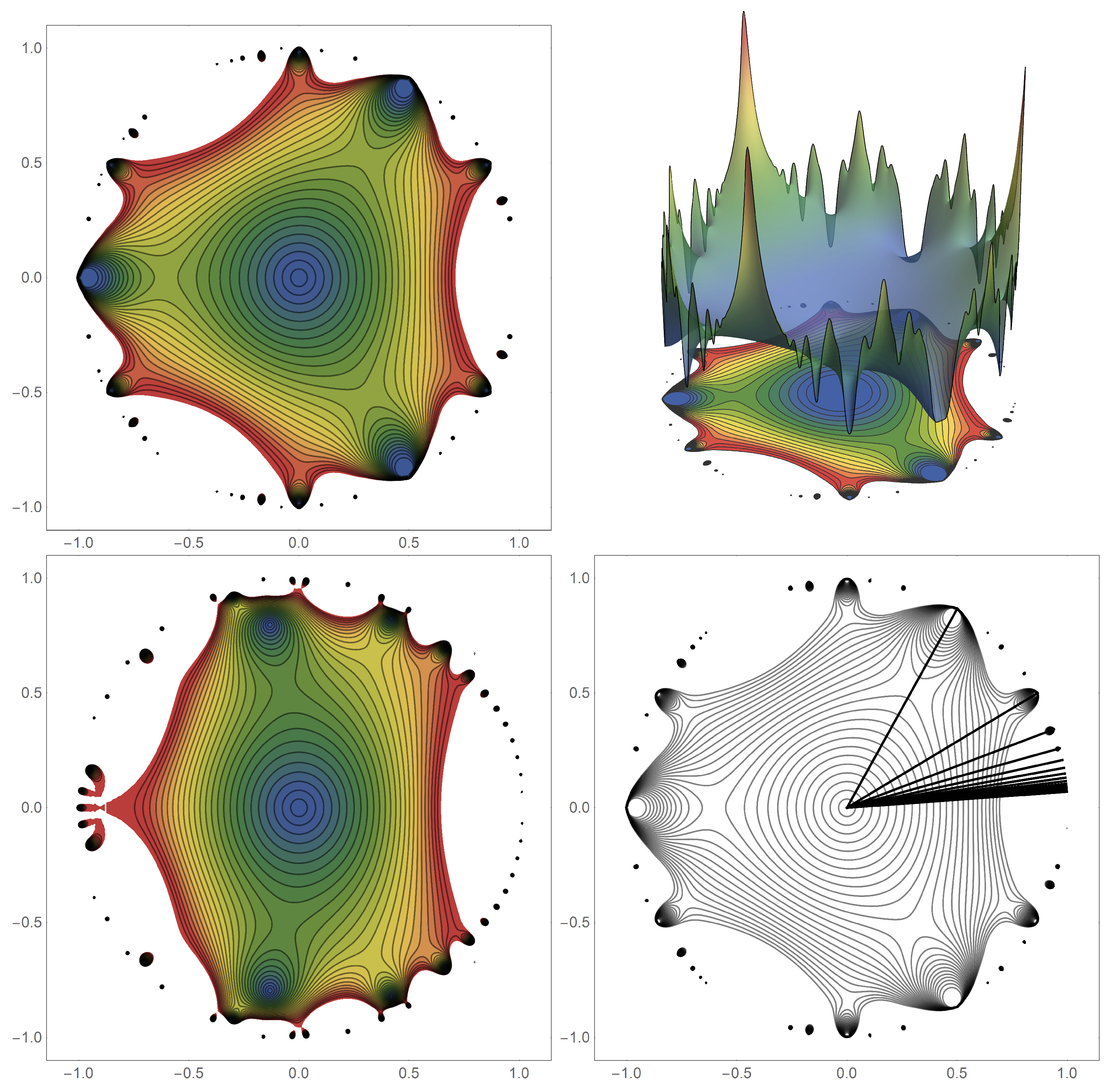
. One particularly important representation of this example function is shown in the bottom left panel of
Figure 1 for the example case of
, the well-known triangular numbers.
Figure 1 shows the modulus of
,
, where the graph is limited to
. That is, the graph is truncated at the unity level set. This is done to better expose the symmetry features of the functions otherwise the divergence at the natural boundary obscures the view of these features.
A
family of note that yields particularly interesting lacunary functions are the centered polygonal numbers. The centered polygonal numbers are a sequence of numbers arising from considering points on an polygonal lattice (see References [
20,
21,
22,
23]). The centered
k-gonal numbers are defined by the formula (for positive integer
)
When is the centered k-gonal number, then is the centered polygonal lacunary function. Also, is the centered polygonal lacunary sequence associated with f.
It turns out that nearly all of the structural features of centered polygonal lacunary functions are independent of the choice of
k (see References [
14,
15]). This is because the centered polygonal numbers are related to the triangular numbers (see Reference [
24]) in a simple way. The set of triangular numbers is
For convenience, lemmas, theorems, and corollaries are proven in Reference [
14] and are stated here without proof. A couple of definitions from Reference [
14] are included as well.
Lemma 1. whereandmean the nth member of the respective sequences. Lemma 2. The sequence of triangular numbers mod p is a-cycle. The sequence is symmetric about the midpoint of the-cycle. Theth member of the-cycle is zero.
Definition 1. Primary symmetry. The rotational symmetry of themember of,, is called the primary symmetry.
Theorem 1. The primary symmetry ofis.
3. The –Sequences
The centered polygonal lacunary functions have very interesting organizational structure at the natural boundary (see References [
14,
15]). Of particular interest are the
p-sequences (see Reference [
14]). These arise when considering the value of the centered polygonal lacunary function on the line segment that runs from the origin to the natural boundary at an angle of
,
. Interestingly, in the limit of
, the sequence
becomes a bounded
cycle of complex numbers (see Reference [
14]).
Definition 2. Symmetry angle. Let the primary symmetry be k-fold. The first symmetry angle is , . The pth symmetry angle is , . The primary symmetry angle is .
At the natural boundary, the
p-sequences have intricate structure (see Reference [
14]) that is a manifestation of Lemma 1. Because of Lemma 2, the values of
oscillate. Further, they take on the value of zero at values of
, where
m is a positive integer. This allows for a convergent sub-sequence which is discussed in
Section 5.
This section concludes with an additional theorem specific to centered polygonal numbers proven here.
Theorem 2. The following rearrangement holds for.whereindicates the floor function. Proof. The identity of Equation (
6) follows directly from the identity
and the well-known quotient-remainder formula,
, where
a,
b,
are any integers. Each term in the summation is then,
Thus Equation (
6) holds and Theorem 2 is proven. □
This theorem has real practical use in that it radically speeds up certain calculations and simplifies certain expressions on MATHEMATICA.
4. Symmetry Angle Spaces
The focus of this work is to restrict the centered polygonal functions, which are analytic on the open complex disk, to a topological space consisting of the union of the line segments lying along the symmetry angles which run from the origin to the natural boundary (located on the unit circle).
Let be the open unit disk in the complex plane and let let be the closed unit disk. Further, one can define for (that, is the line segment along the pth symmetry angle, . One likewise define the closure of as , where now .
The symmetry angle space is then defined as
and its closure,
Note that as
p approaches
∞ the symmetry line approaches the real axis. Thus one needs to consider a second type of closure. If the real line is included, one denotes the subspaces as
and
.
Thus, there are four related subspaces upon which the centered lacunary functions are restricted:
,
,
, and
. These subspaces are related to the so-called broom topological spaces (see Reference [
17]). They naturally take on a subspace topology, that is the normal topology for a line segment. All four of these subspaces are arc-connected and, in fact, star-connected through the origin. In
Section 7, subspaces
,
,
, and
are homeomorphically mapped to longitudinal lines of the sphere. This allows for closed form expressions for integrals of
along paths in these mapped spaces.
5. Cyclic Decomposition
Along the symmetry angle, the resultant
p-sequence has a
cycle, and, in fact, the
cycle further breaks into a
-cycle at the modulus level as discussed in
Section 3. Finally, by Lemma 2 the
member of the the
cycle is zero. Because of this, it is natural to consider a subset of
for which
,
; call this subsequence
. For every member of this subsequence
is zero.
One can express the
jth cycle as
where
j is any non-negative integer. Thus, the full function can be decomposed into the cyclic summations,
Figure 2 shows the cyclic summation decomposition of
for the examples of
and
. The fundamental component,
, captures much of the full function, but deviates significantly as
. The actual peak occurs at
. An inspection of
Figure 2 shows that
increases with increasing
k as the curves are skewed towards the natural boundary.
The higher components
contribute very little for low values of
. Each of the subsequent higher components begin to make significant contributions to the full function closer and closer to the natural boundary. One notices in
Figure 2 that both the real (blue curve in figure) and imaginary (red curve) parts of the component cyclic summations alternate signs.
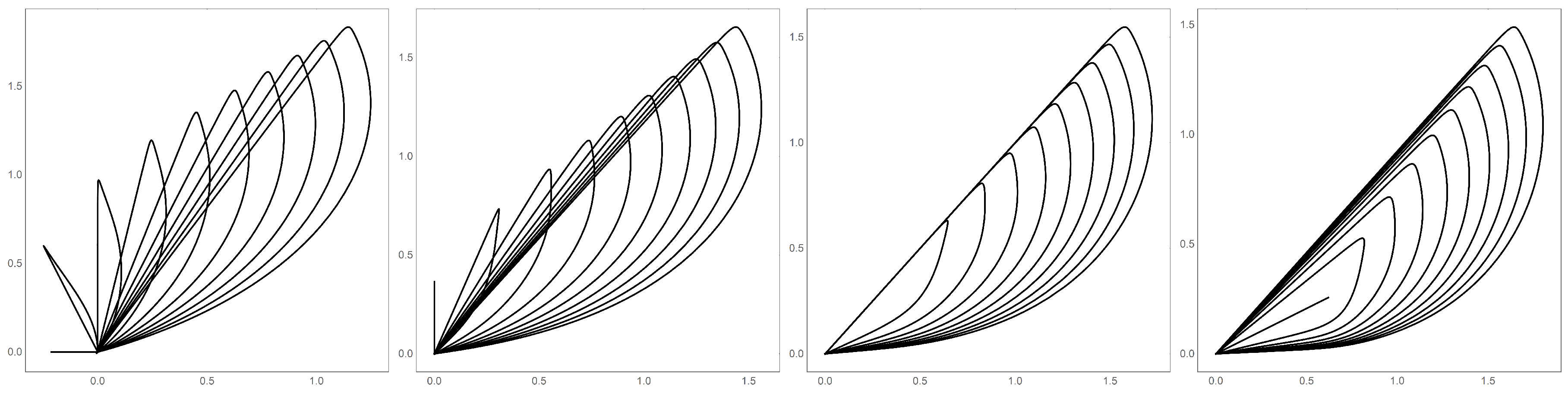
Figure 3 shows cyclic decompositions for the centered polygonal lacunary functions along the line segments at
for several different values of
k.
6. Parametric Curves
The centered polygonal lacunary functions on
can be represented in a visually instructive way via the parametric curves:
The parametric curves for
are shown in
Figure 4. Here values of
are shown for each
k. (Note,
is plotted in an auxiliary
plane, not in the original complex plane containing
.)
The most obvious feature is that these produce a closed curve in the plane starting at the origin for
and returning to the origin for
. Note that the curves
are all degenerate meaning that the encircled area is zero. Higher values of
p give rise to larger and larger enclosed areas (
Figure 4). Hand-in-hand with increasing area is increasing arclength which is also shown in
Figure 4 and
Figure 5.
A more subtle view of the closed curves reveals an “acceleration” with
and this acceleration increases with increasing
p. The “velocity” is represented as red tangent vectors in
Figure 5. One notices a slow acceleration along the lower arc of the curve (for
). Acceleration then rapidly increases at the apex of the curve and along the return path (
). The change in acceleration at the apex corresponds to an abrupt change in arclength with
(see the bottom left panel of
Figure 5). An incidental observation regarding arclength is that it closely fits an empirical curve of the form
regardless of
k (see bottom right panel of
Figure 5).
Perhaps more interesting, however, is the geometrical behavior of the curves. The initial angle of the curve at is . This is intuitive and quick to prove.
Theorem 3. The initial angle ofis.
Proof. One can make use of the fact that for small
,
is dominated by the first term in the sum. This goes as
The asymptotic form as
is
The phase is
, which completes the proof. □
Less intuitive is the behavior of the return angle as . First after the curve is nearly a straight line. Further, the angle of that line is for , but, interestingly, it asymptotically goes to as . The return angle becomes independent of k. The proof of this statement is probabilistic in nature and is wanting of a more rigorous proof.
Theorem 4. The return angle offoris.
Proof. From Theorem 2 and
, one has
Now, from Equation (
3)
and
So this reduces
to
The sum is now pure real and setting
. Hence, the return angle is
. □
Conjecture 1. For p a positive integer, Remark 1. The proof is subtle and an analytic one remains elusive. Nonetheless, the conjecture is understandable on probabilistic grounds. Unfortunately, the limit ofis not helpful since the function is identically zero and information about the approach angle is lost. As opposed to the case of, the case ofnow activates many terms in the summation of. In betweenand 1 there is not equal weighting of the terms in the cyclic summation, but the weights of the higher terms are no longer negligible. Thus, the limit is a (non-zero) weighted average of many terms. For large p values, the weighed average of manyultimately gives rise toand, hence, the return angle is.
Because these parametric curves produce enclosed regions, the area within the curves can be calculated. This area is found through a numerical integration of the curve, however the area of every value of
k for
will be zero, as the parametric graph of
is a straight line.
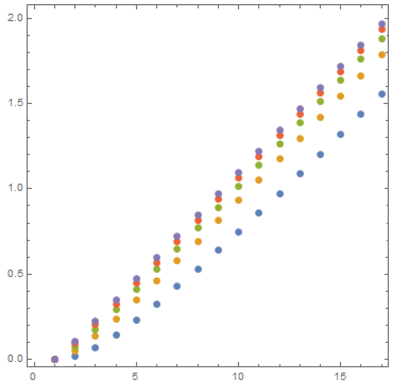
Figure 6 is a graph of the area of the associated parametric curves for
and
. Each set of points shows the area for a distinct
k value, with the bottom set being the area of
, and the top being the area of
. As the
p value increases a linear trend appears, however the equation for what
p approaches to does not seem to have a general trend.
7. Whole Sphere Mapping
Due to the natural boundary of the centered polygonal lacunary functions sitting on the unit circle in the complex plane, there is no reason to consider the domain outside of the closed disk. There is an interesting and convenient mapping that maps the disk to , which is embedded in as the unit sphere centered at the origin, such that the entire unit circle is mapped to the south pole (). As will be seen, this, in some sense, compresses the natural boundary to an isolated singularity. Further, the symmetry angle spaces map to longitudinal arcs and, given the nature of the p-sequences, this singularity is, again in some sense, removed.
Specifically, the above map is a parametric mapping that will take point,
from
into
, such that the set of all points in
cover the unit sphere centered at the origin. It is convenient to use spherical polar coordinates to describe the parametric surface. This is done with the identification,
With this identification,
is expressed as a function of the zenith angle (
) from spherical polar coordinates,
. Likewise,
in the complex plane corresponds directly to azimuthal angle (
) of spherical polar coordinates. The parametric mapping on
, which is embedded in
parametrically as
, can be written as
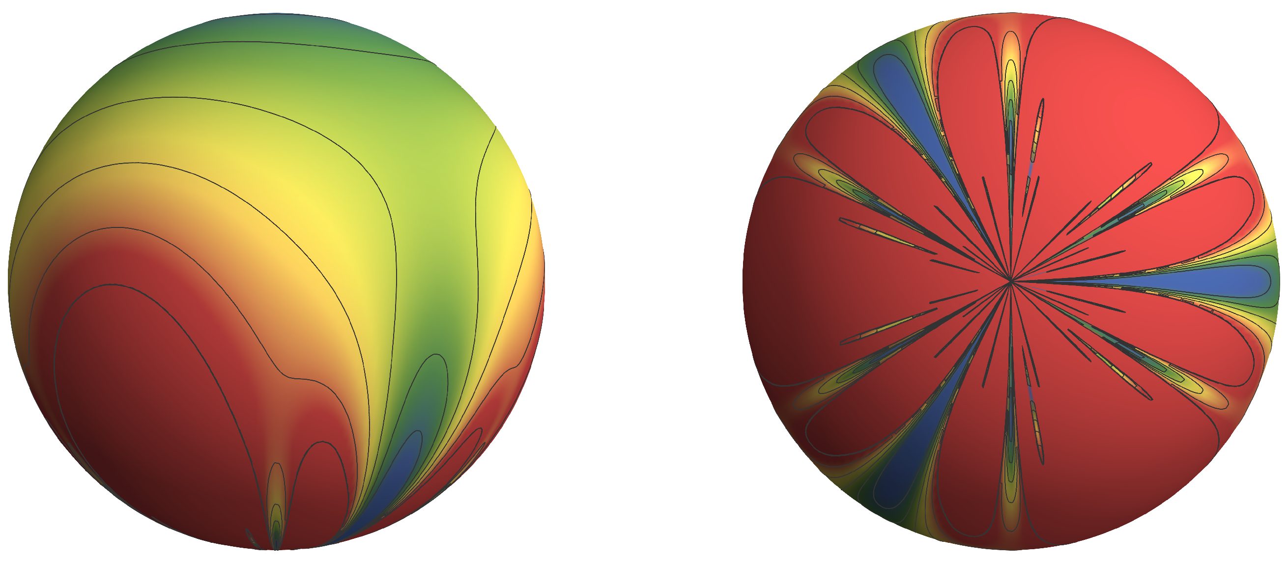
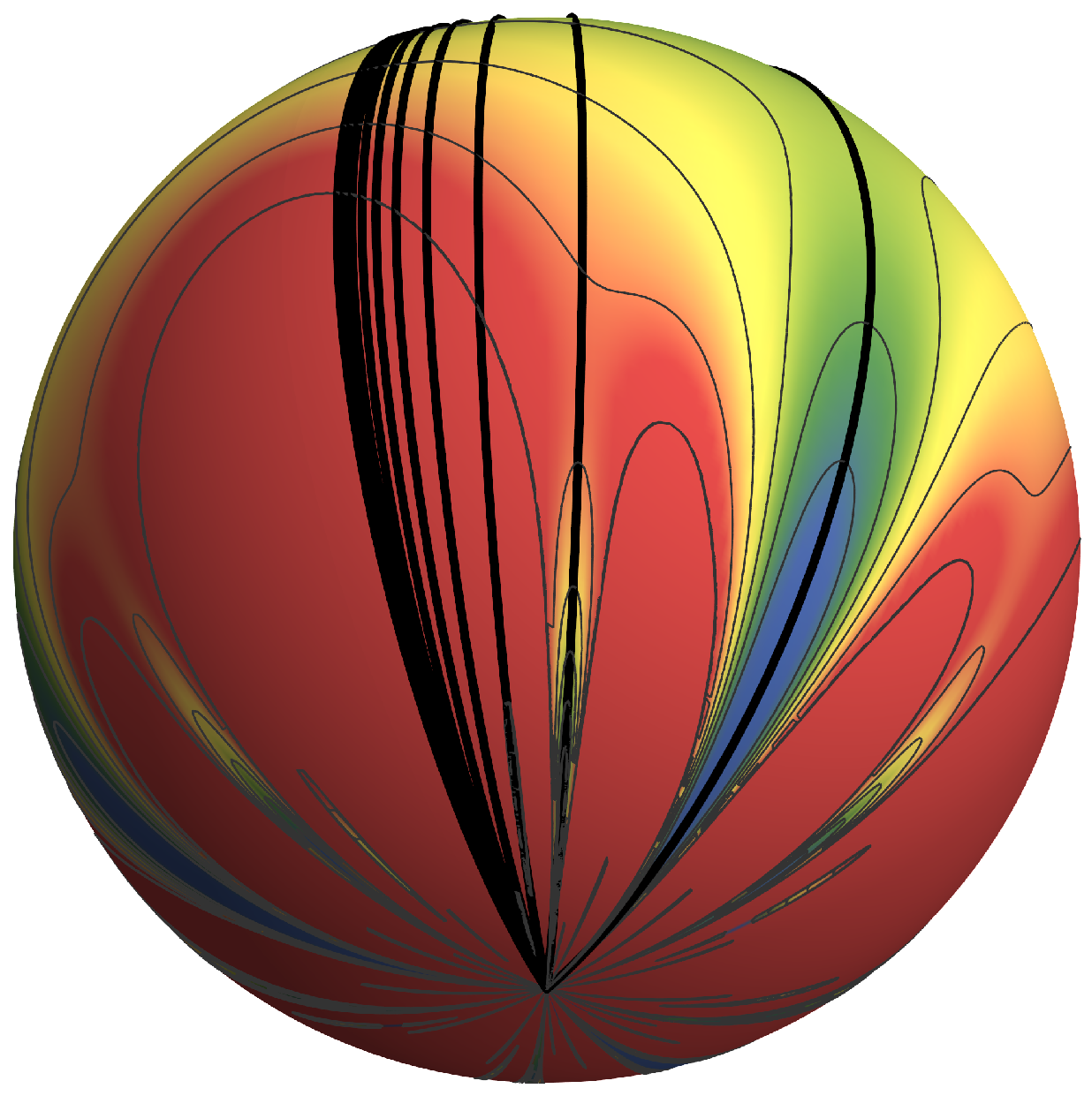
Under this mapping,
becomes
. The example of
is shown in
Figure 7. The mapping is that of the centered polygonal lacunary function shown in the upper left panel of
Figure 1. So the centered polygonal functions is the wrapped over the sphere such that the natural boundary gets pinched into the south pole.
Then the restriction to, for example,
induces the map
Here
is the restricted domain of longitudinal arcs; an example is shown in
Figure 8.
(as well as
) are star-connected through both the north pole (origin) and south pole (contracted unit circle). Because of this, one can define loops on
and
, with the north pole as the base-point, that traverse one longitudinal arc
and return along another
. The fundamental group (in the homotopy sense) is
, where ∗ is the loop product, that is, the concatenation of loops [
18].
The spaces
and
offer an interesting opportunity to explore closed-loop path integrals of
. Call the path along the
p symmetry angle running from the north pole to south pole in
,
. Then a closed-loop can be obtained by considering
. The integral along
is expressed as
The second factor accounts for the appropriate integration metric along angle
. This integral can be evaluated and one has the following theorem.
Theorem 5. Let k, m, p be any positive integers and let. Then, Proof. Now, Equation (
23) is
Expressing
in summation form and interchanging the summation and the integration gives
Using,
the integral is quickly evaluated.
where
and
were expressed in their functional form as well as expressing
. □
Conjecture 2. Let k and m be positive integers and,This can also be written aswhereis the digamma function (see Reference [25]) and. Remark 2. When, Equation (28) becomesThis summation yields to a closed form which is Equation (29) (see Reference [19]). Using the relations for the digamma function built in to MATHEMATICA, this simplifies to Equation (30) (see Reference [19]). The digamma function has many applications in physics and even in the life sciences (see the review by Hăşmăşanu et al. [
26])
versus
k is shown in
Figure 9.
approaches a
k-dependent limit value.
Corollary 1. Let k, m, p be positive integers and. Then, on,where. Proof. Beginning with the summation formula of the tangent function,
(see Reference [
25,
27]), and
. Starting with the right hand side of Equation (
32),
Simplify and manipulating gives,
This completes the proof. □
Corollary 2. Let k be a positive integer, thenand
Proof. The proof follows from Equations (
30) and (
32) by first making a change of variable
. Upon doing this and performing a bit of algebraic simplification, Equation (
30) becomes
One can then expand this expression in a Taylor series about
to get
Which in the limit of
becomes
.
By a similar procedure, Equation (
32) becomes
Series expansion gives
which, again is
in the limit of
. □
Based on Corollary 2 the following unproven conjecture is proposed.
Conjecture 3. Let k be a positive integer, then
Remark 3. is special and Equations (30) and (32) must be evaluated using limits ofand L’Hospital’s rule. When, Equation (30) becomesand Equation (32) becomes. The closed-loop integral is then on
and
,
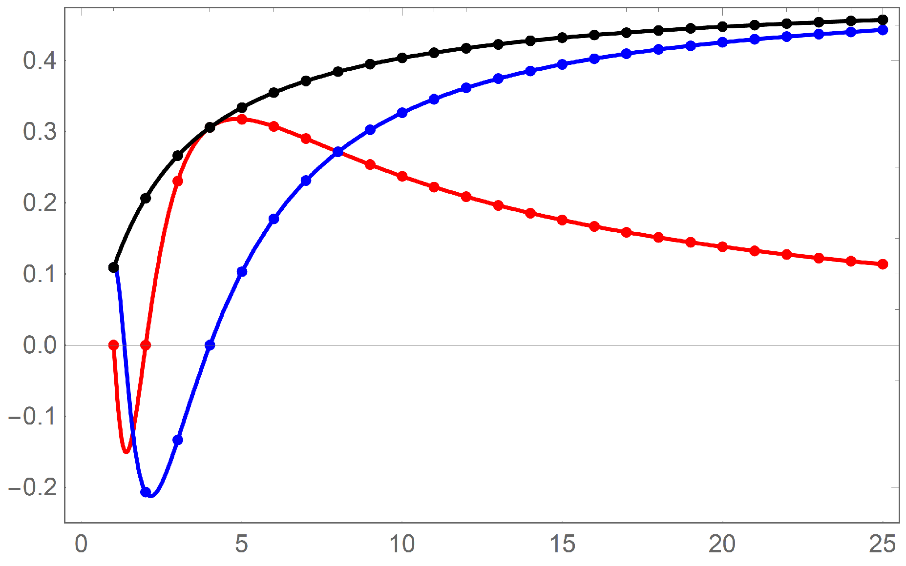
Of special interest is
, where the return path is along
. The left panel of
Figure 10 shows the behavior of
for
through
and
. A finite limiting values is reached for
. It is natural to consider a normalized version of
to compare different values of
k. This is done by multiplying by
and a graph is shown in the right panel of
Figure 10. The dashed line in the figure represent the limiting value of
as
as given by the following theorem.
Theorem 6. Let k be any positive integer. On, Proof. One considers
(c.f., Equations (
30) and (
32)) and uses the same strategy as in the proof of those expressions. Change of variable
and simplification gives,
And series expansion yields
Thus the limit as
is
. □
8. Conclusions
This work focused on the centered polygonal lacunary functions restricted to symmetry angle space. The periodicity of the p-sequences and the existence of a convergent subsequence provided a framework for decomposition of the centered polygonal lacunary functions. This decomposition could be potentially useful in renormalization procedures as one approaches the natural boundary.
The surjective spherical mapping of the unit disk such that the natural boundary is mapped to the south pole was useful in investigating line integrals of the centered polygonal lacunary functions. Closed form functional representations were achieved in some cases.
It is hoped that this work provides useful insight into the nature of the natural boundary of centered polygonal lacunary functions, both on the full unit disk and also restricted to symmetry angle space. Statistical mechanics is the most promising link of this work to physics. This is for two reasons. First is simply a counting application, for example, the canonical partition function. Second is the self-similarity of these functions and the possible use in renormalization schemes applied to phase transitions. Optics may be the closest experimental link either via simple signal processing scheme or, more interestingly, in application to, for example the Talbot effect or other such phenomena.


