Article

Optimum Design of Infinite Perforated Orthotropic and Isotropic Plates

by
Mohammad Jafari
1,
Seyed Ahmad Mahmodzade Hoseyni
1,
Holm Altenbach
2 and
Eduard-Marius Craciun
3,*
1
Faculty of Mechanical and Mechatronics Engineering, Shahrood University of Technology, P.O. box 3619995161 Shahrood, Iran
2
Lehrstuhl für Technische Mechanik, Institut für Mechanik, Fakultät für Maschinenbau, Otto-von-Guericke-Universität Magdeburg, 39106 Magdeburg, Germany
3
Faculty of Mechanical, Industrial and Maritime Engineering, Ovidius University of Constanta, 900527 Constanta, Romania
*
Author to whom correspondence should be addressed.
Mathematics 2020, 8(4), 569; https://doi.org/10.3390/math8040569
Submission received: 6 March 2020 / Revised: 30 March 2020 / Accepted: 7 April 2020 / Published: 11 April 2020
(This article belongs to the Special Issue Applied Mathematics and Solid Mechanics)

Abstract

:
In this study, an attempt was made to introduce the optimal values of effective parameters on the stress distribution around a circular/elliptical/quasi-square cutout in the perforated orthotropic plate under in-plane loadings. To achieve this goal, Lekhnitskii’s complex variable approach and Particle Swarm Optimization (PSO) method were used. This analytical method is based on using the complex variable method in the analysis of two-dimensional problems. The Tsai–Hill criterion and Stress Concentration Factor (SCF) are taken as objective functions and the fiber angle, bluntness, aspect ratio of cutout, the rotation angle of cutout, load angle, and material properties are considered as design variables. The results show that the PSO algorithm is able to predict the optimal value of each effective parameter. In addition, these parameters have significant effects on stress distribution around the cutouts and the load-bearing capacity of structures can be increased by appropriate selection of the effective design variables. The main innovation of this study is the use of PSO algorithm to determine the optimal design variables to increase the strength of the perforated plates. Finite element method (FEM) was employed to examine the results of the present analytical solution. The results obtained by the present solution are in accordance with numerical results.

1. Introduction

Nowadays, the design of metal and composite plates with cutouts is of a great importance due to their extensive application in different industries [1,2]. It is well known that, due to geometric changes in different structures, highly localized stresses are created around discontinues areas, at which structural failure usually occurs [3]. Therefore, the analysis of this phenomenon, called stress concentration, has a significant importance for designers of engineering structures. The fracture strength of these structures depends strongly on the stress concentration caused by cutouts. Stress concentration and fracture criterions are very important in evaluating the reliability of engineering structures [4]. For instance, designing vehicles with the purpose of weight reduction in order to decrease fuel consumption and utilize engines with less power are some applications of these plates. In this study, according to the extensive usage of different types of cutouts and considering a long process of trial and error to find their optimum design, particle swarm optimization (PSO) algorithm (see, e.g., [5]) is employed for the integrity of the search process in obtaining the optimum design. The main innovation of this paper is the use of PSO algorithm to determine the optimal design variables to increase the strength of the perforated plates.

2. Literature Review

Complex potential method established by G.V. Kolosov and N.I Muskhelishvili (see, e.g., [6,7,8]) has been applied for anisotropic plates by Green and Zerna [7], Lekhniskii [9], Sih et al. [10], Lekhniskii [11], Bigoni and Movchan [12], Radi et al. [13], Craciun and Soós [14], Craciun and Barbu [15], and Chaleshtari and Jafari [16]. Tsutsumi et al. [17] investigated the solution of a semi-infinite plane with one circular hole. Their solution was based on repeatedly superposing the solution of an infinite plane with one circular hole and of a semi-infinite plane without holes to eliminate the stresses arising on both boundaries. Applying Lekhnitskii’s method [9,11], Rezaeepazhand and Jafari [18] presented an analytical solution for the stress analysis of orthotropic plates with different cutouts and evaluated the stress distribution around a quasi-square cutout in orthotropic plates. They studied the effect of various parameters such as load angle, fiber angle, and cutout orientation for perforated orthotropic plates. Yang et al. [19] presented an analytical solution for the stress concentration problem of an infinite plate with a rectangular cutout under biaxial tensions. Rao et al. [20] found stress distribution around square and rectangular cutouts using Savin’s formulation [6]. Sharma [21] used Mushkhelishvili’s complex variable approach [8] and presented the stress field around polygonal shaped cutouts in infinite isotropic plates. The effect of cutout shape, bluntness, load angle, and cutout orientation on the stress distribution was studied for triangular, square, pentagonal, hexagonal, heptagonal, and octagonal cutout shapes. Banerjee et al. [22] studied stress distribution around the circular cutout in isotropic and orthotropic plates under transverse loading using three-dimensional finete element models created in ANSYS. They investigated the effects of plate thickness, cutout diameter, and material on the amount of stress concentration in orthotropic plates. Marin et al. [23] studied the structural stability of an elastic body with voids and straight cracks in dipolar elastic bodies. Using the method of singular integral equations (see, e.g., [24]), Kazberuk et al. [25] presented the stress distribution in the quasi-orthotropic plane weakened by semi-infinite rounded V-notch.
Optimal structures with irregular geometry but with simple fields inside were investigated by Vigdergauz [26,27,28], Grabovsky and Kohn [29,30], Vigdergauz [31,32,33]. The related problem of an optimal shape of a cavity in an elastic plane was considered by Cherepanov [34], Banichuk [35], Banichuk and Karihaloo [36], Banichuk et al. [37], Vigdergauz and Cherkayev [38], Vigdergauz [28], Markenscoff [39], and Cherkaev et al. [40]. In addition, Cherepanov [34,41] proposed an effective exact solution of some inverse plane problems of the theory of elasticity concerning the determination of equally strong outlines of holes. Sivakumar et al. [42] studied the optimization of laminate composites containing an elliptical cutout by the genetic algorithm (GA) method (see, e.g., [43]). In this research, design variables were the stacking sequence of laminates, thickness of each layer, the relative size of cutout, cutout orientation, and ellipse diameters. The first and second natural frequencies were considered as a cost function. Cho and Rowlands [44] showed GA ability to minimization of tensile stress concentration in perforated composite laminates. Chen et al. [45] used a combination of PSO and finite element analysis to optimize composite structures based on reliability design optimization. Zhu et al. [46] considered the optimization of composite strut using the GA method and Tsai–Wu failure criterion [47]. They paid attention to minimizing the weight of the structure and increasing the buckling load. Fiber volume fraction and stacking sequence of laminates were considered as design variables. Artar and Daloğlu [48] used the GA to determine the optimum variable to achieve suitable steel frames. Moussavian and Jafari [49] calculated the optimal values of effective parameters on the stress distribution around a quasi-square cutout using different optimization algorithms such as Particle Swarm Optimization (PSO), GA, and Ant Colony Optimization (ACO) [50]. To achieve this goal, the analytical method based on Lekhnitskii’s method was employed to calculate the stress distribution around a square cutout in the symmetric laminated composite. Jafari and Rohani [51] studied the optimization of perforated composite plates under tensile stress using GA method. The analytical solution was used to determine the stress distribution around different holes in perforated composite plates. Using GA, Jafari and Hoseyni [52] introduced the optimum parameters in order to achieve the minimum value of stress around different cutouts. Vosoughi and Gerist [53] proposed a hybrid finite element (FE), PSO, and conventional continuous GA (CGA) for damage detection of laminated composite beams. The finite element method (FEM) was employed to discretize the equations. Their design variables were damage ratios, the number of damaged elements, and the number of layers. Manjunath and Rangaswamy [54] optimized the stacking sequence of composite drive shafts made of different materials using PSO. The optimum results obtained by PSO are compared with results of GA and found that PSO yields better results than GA. Ghashochi Bargh and Sadr [55] used the PSO algorithm to the lay-up design of symmetrically laminated composite plates for maximization of the fundamental frequency. The design variables were the fiber orientation angles, edge conditions, and plate length/width ratios. Several algorithms are valid alternatives to PSO. Some of these alternatives are not heuristic algorithms but they have a strong theory behind them [56,57,58].
This paper aims to introduce a suitable mapping function and optimal cutout geometry in the perforated orthotropic plate under uniaxial tensile loads, biaxial loads, and shear loads. The design variables are cutout orientation, the aspect ratio of the cutout, bluntness, load angle, and fiber angle. Minimizing normalized stress around the cutout the Tsai–Wu criterion is considered as a cost function of the particle swarm optimization algorithm. The normalized stress is the ratio of the maximum value of circumferential stress at the edge of the cutout to the nominal or applied stress, which is called stress concentration factor (SCF).

3. Theoretical Formulation

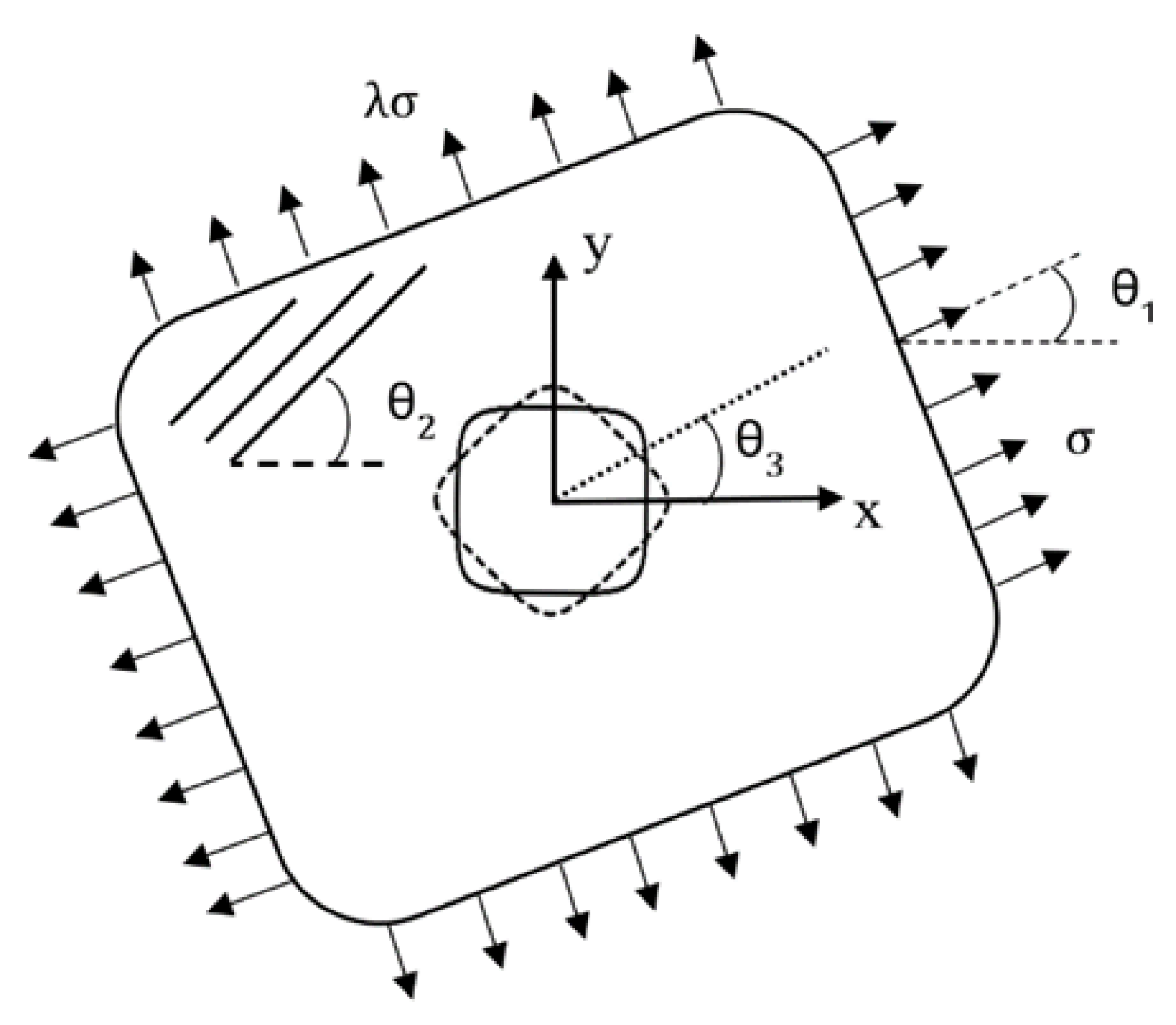
The problem studied in this paper is an infinite plate containing a quasi-square cutout. As shown in Figure 1, the plate is under biaxial loading at an angle θ 1 (load angle) with respect to the x-axis. The square cutout has arbitrary orientations such that its major axis is directed at an angle θ 3 (rotation angle) with respect to the x-axis and fiber angle is θ 2 [59]. In this paper, the stress function is converted to an analytical expression with undetermined coefficients and displacements, and stresses can be calculated by stress function being determined. In this case, it is assumed that the plate has a linear elastic behavior. Because of the traction-free boundary conditions on the cutout edge, the stresses σ ρ and τ ρ θ at the cutout edge are zero and the circumferential stress σ θ is the only remaining stress. The equilibrium equations are satisfied by introducing F ( x , y ) as stress function [60,61,62] according to Equation (1)
σ x = 2 F y 2 , σ y = 2 F x 2 , τ x y = 2 F x y .
The orthotropic stress–strain relation for plane problems in terms of the components of the reduced compliance matrix is as follows [62]:
ε x = R 11 σ x + R 12 σ y ε y = R 12 σ x + R 22 σ y τ x y = R 66 τ x y .
The constitutive vector-matrix equation of a orthotropic material in the global coordinate system is as follows [62]:
ε x ε y ε z γ y z γ x z γ x y = S 11 S 12 S 13 0 0 0 S 12 S 22 S 23 0 0 0 S 13 S 23 S 33 0 0 0 0 0 0 S 44 0 0 0 0 0 0 S 55 0 0 0 0 0 0 S 66 σ x σ y σ z τ y z τ x z τ x y
where S i j are the components of the orthotropic compliance matrix. The inverted relation is [62]
σ x σ y σ z τ y z τ x z τ x y = C 11 C 12 C 13 0 0 0 C 12 C 22 C 23 0 0 0 C 13 C 23 C 33 0 0 0 0 0 0 C 44 0 0 0 0 0 0 C 55 0 0 0 0 0 0 C 66 ε x ε y ε z γ y z γ x z γ x y
with the components of the stiffness matrix C i j . The transform rules for S i j into C i j and vice versa are presented in [62].
For plane stress state, σ z = τ x z = τ y z = 0 is assumed, which means the last equation is degenerated to
σ x σ y 0 0 0 τ x y = C 11 C 12 C 13 0 0 0 C 12 C 22 C 23 0 0 0 C 13 C 23 C 33 0 0 0 0 0 0 C 44 0 0 0 0 0 0 C 55 0 0 0 0 0 0 C 66 ε x ε y ε z γ y z γ x z γ x y .
It is obvious that, if the shear stresses τ x z = τ y z = 0 , the conjugated strain must be zero if we have orthotropic material behavior. Finally, the remaining part of the last equation is
σ x σ y 0 τ x y = C 11 C 12 C 13 0 C 12 C 22 C 23 0 C 13 C 23 C 33 0 0 0 0 C 66 ε x ε y ε z γ x y .
Thus, we have three constitutive equations and one constraint
C 13 ε x + C 23 ε y + C 33 ε z = 0
or
ε z = C 13 C 33 ε x + C 23 C 33 ε y .
The strain ε z can now be substituted in the expressions for σ x
σ x = C 11 ε x + C 12 ε y C 13 C 13 C 33 ε x + C 23 C 33 ε y
and finally we get
σ x = C 11 C 33 C 13 2 C 33 ε x + C 12 C 33 C 13 C 23 C 33 ε y .
In a similar manner, σ y can be expressed. The equations for both stresses can be solved with respect to the strains ε x and ε y and finally the reduced compliance components can be computed.
By replacing stress–strain relations in compatibility relation, we obtain
2 ε y x 2 + 2 ε x y 2 = 2 2 ε x y x y
and rewriting the resultant equation in terms of stress function, the compatibility equation for orthotropic material yields:
R 11 4 F y 4 + ( 2 R 12 + R 66 ) 4 F x 2 y 2 + R 22 4 F x 4 = 0 .
Lekhniskii [60] showed that this equation can be transferred to four linear operators of first order D k :
D 1 D 2 D 3 D 4 F ( x , y ) = 0 , D k = y μ k x ,
and we obtain the characteristic equation as follows
R 11 μ 4 + ( 2 R 12 + R 66 ) μ 2 + R 22 = 0 .
It can be proved, in general, that Equation (5) has four complex conjugate roots ( μ 1 = μ 2 = ± i , μ 1 ¯ = μ 2 ¯ = ± i ) and the general expression for the stress function is:
F ( x , y ) = 2 [ φ ( z 1 ) + ψ ( z 2 ) ] ,
where [ ] indicates the real part of the expression inside the brackets and z k = x + μ k y and μ k , k = 1 , 2 are the roots of the characteristic equation of anisotropic materials.
Finally, the stress components in terms of two potential functions of φ ( z 1 ) and ψ ( z 2 ) are expressed [52]:
σ x = σ x + 2 [ μ 1 2 φ ( z 1 ) + μ 2 2 ψ ( z 2 ) ] , σ y = σ y + 2 [ φ ( z 1 ) + μ 2 2 ψ ( z 2 ) ] , τ x y = τ x 2 [ μ 1 φ ( z 1 ) + μ 2 ψ ( z 2 ) ]
where
σ x = σ 2 [ ( λ + 1 ) + ( λ 1 ) cos 2 θ 1 ] , σ y = σ 2 [ ( λ + 1 ) ( λ 1 ) cos 2 θ 1 ] , τ x y = σ 2 [ ( λ 1 ) sin 2 θ 1 ]
with σ as applied load (see Figure 1). In the above-presented equations, by taking appropriate values of λ describing the type of loading and θ 1 for stress applied at infinity ( σ x , σ y , τ x y ) , uniaxial loading, equibiaxial loading, and shear loading can be considered. The following values of λ and θ 1 may be taken into Equation (8) to obtain various cases of in-plane loading:
  • inclined uniaxial tension: λ = 0 and θ 1 0 ;
  • equibiaxial tension: λ = 1 and θ 1 = 0 ; and
  • shear loading: λ = 1 and θ 1 = π 4 , 3 π 4 .
We denote by φ ( z 1 ) , ψ ( z 2 ) the derivatives of the functions φ ( z 1 ) and ψ ( z 2 ) with respect to z 1 and z 2 . These analytic functions can be determined by applying the boundary conditions. To calculate the stress components in the polar coordinates system, we use the following equations
σ θ + σ ρ = σ y + σ x
σ θ σ ρ + 2 i τ ρ θ = ( σ y + 2 i τ x y ) e 2 i Ω .
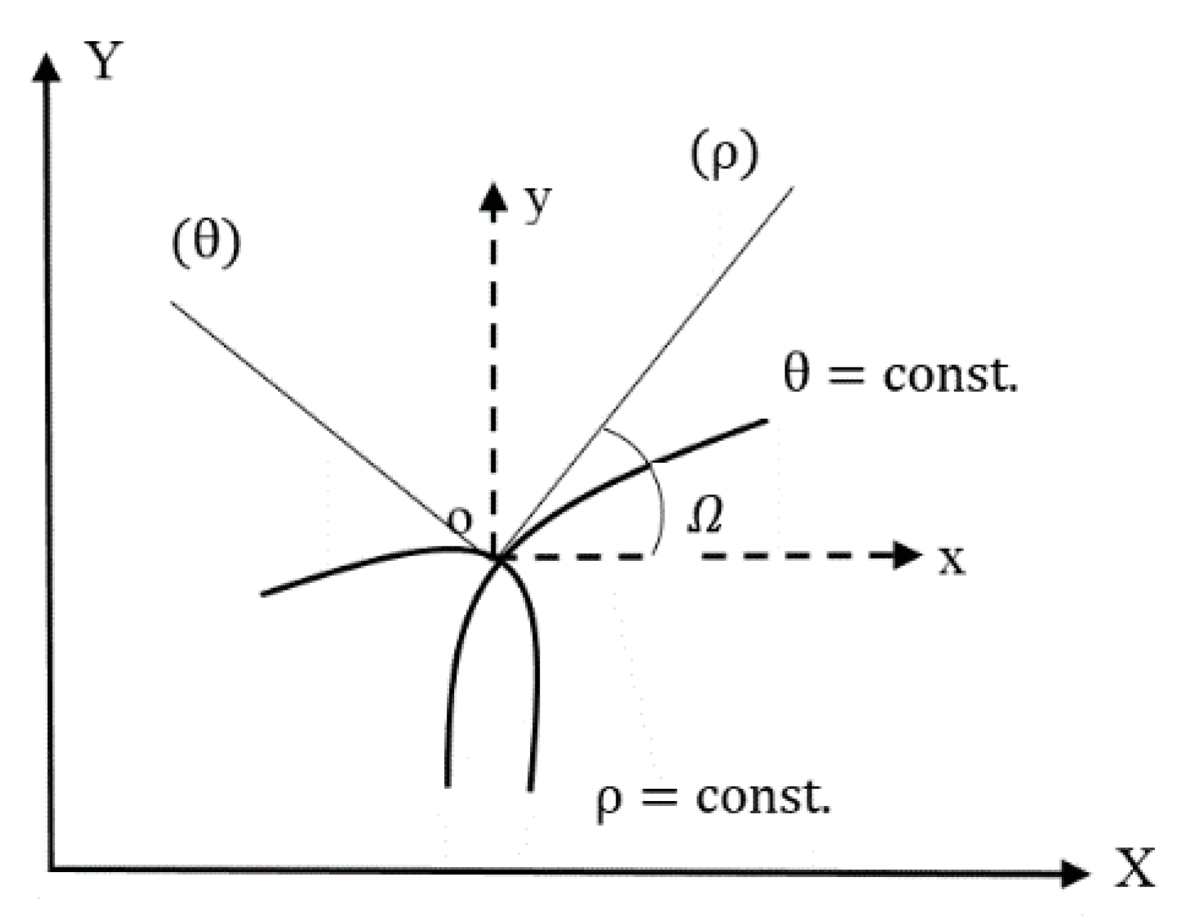
In these equations, Ω is the angle between the positive x-axis and the direction ρ (Figure 2).

4. Conformal Mapping

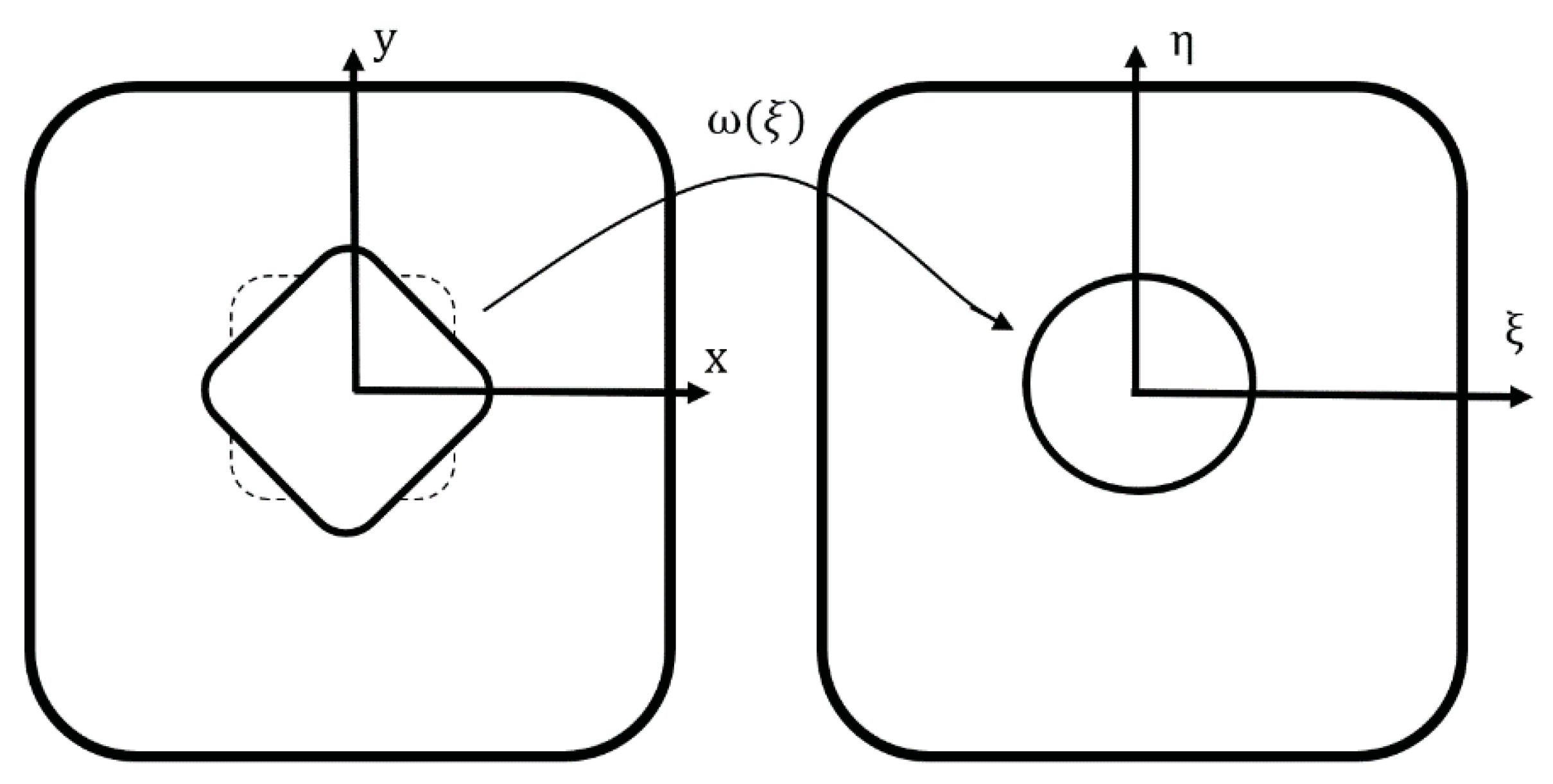
To apply the Lekhnitskii’s method to quasi-square cut out, establishing a relation between the cutout and a circular cutout is necessary [63]. A conformal mapping can be used to map the external area of a quasi-square cutout in z-plane into the area outside the unit circle in ξ -plane (Figure 3). Such a mapping function is represented thus:
z = ω ( ξ ) = x + μ k y ,
where x and y are obtained as follows:
x = ( cos θ + w cos n θ ) ,
y = c ( sin θ w sin n θ ) .
The parameter w determines the bluntness factor and changes the radius of curvature at the corner of the cut out (Figure 4).
As can be concluded from Equations (12) and (13), w = 0 presents the circular cutout. Integer n in the mapping function represents the shape of the cutout. The cutout sides are given by n + 1 . Bluntness w and cutout orientation θ 3 are important parameters that influence the stress distribution around the different cutouts. Parameter c is the aspect ratio of cutout (length/width ratio) and Figure 5 shows the good effects of these parameters on the cutout geometry. With increasing of c at a constant value of w, the cutout is elongated in one direction. For circular and elliptical cutout, c = 1 and c 1 , respectively, and, for both cases, w is equal to zero. For an elliptical cutout, c is the ratio of diameters the ellipse ( c = b / a ) , where a and b are semi-major and semi-minor axis of the ellipse, respectively.

5. Particle Swarm Optimization

Particle Swarm Optimization (PSO) is a population-based stochastic search optimization algorithm [64,65]. This algorithm starts to work with a number of initial answers which are determined randomly, and it looks to find an optimum answer by moving these answers through consecutive iterations. In each iteration, the position of each particle in the search space is determined based on the best position obtained by itself and the best position obtained by the whole particles during the searching process. In each iteration, the particles, velocities and particle position are updated according to Equations (14) and (15), respectively [66],
V i ( t + 1 ) = ω V i ( t ) + r 1 c 1 [ P i ( t ) X i ( t ) ] + r 2 c 2 [ p i ( t ) X i ( t ) ] ,
X i ( t + 1 ) = X i ( t ) + V i ( t + 1 ) ,
where V i ( t ) and X i ( t ) are the current velocity and position of the particle respectively. Let X i ( t ) = { x 1 ( t ) , , x N v a r ( t ) } be the position of particle in a N var -dimensional search space at iteration t. We denote by X i ( t + 1 ) and V i ( t + 1 ) the updated velocity and position, respectively, and by ω the inertia weight coefficient that controls the exploration and exploitation of the search space. c 1 and c 2 are two positive constants called the cognitive and social coefficients, respectively. A high inertia weight causes the available particles in the algorithm to search newer areas and perform a global search. On the contrary, the low inertia weight leads the particles to stay in a limited area. When the value of c 1 increases, the particles tend to move toward the best individual experience and their motion toward the best group’s experience decreases, whereas, by increasing the c 2 , the particles move toward the best group’s experience, thus their motion toward the best individual experience decreases. Let r 1 , r 2 [ 0 , 1 ] be two random numbers, and P i ( t ) and p i ( t ) are the best individual and group’s experiences position, respectively. Choosing the appropriate values for c 1 , c 2 , and ω results in an acceleration in convergence and leads to find the absolute optimum and prevents premature convergence in a local optimum. Here, c 1 and c 2 parameters update as in Equation (16) where c 1 , f , c 2 , f , c 1 , i , and c 2 , i are constant values. In addition, Equation (17) is considered for ω operator where ω i and ω f are initial and final values of weight factor, respectively; I is the number of particle’s current iteration; and I max is the number of the greatest iteration [67].
c 1 = ( ω i ω f ) I I max + c 1 , i , c 2 = ( c 2 , f c 2 , i ) I I max + c 2 , i ,
ω = ( ω i ω f ) I max I I max + ω f .
In a N var -dimensional problem, a particle includes a row vector with N var elements. This arrangement is defined as
P = [ p 1 , p 2 , , p N v a r ] .
To begin the algorithm, a number of these particles (as the number of the primary particle algorithm) must be created.
The failure criterion and SCF are taken as a cost function (C.F.) for orthotropic and isotropic plate, respectively. It should be mentioned that, in [41,68], an alternative approach is presented. SCF is defined as the ratio of the von Mises stress, which is the maximum value of circumferential stress at the edge of the cutout ( σ θ ) , to the nominal or applied stress. In the case of a composite lamina, the strength is calculated by using the Tsai–Wu criterion:
Cost Function C . F . = SCF = min σ f 2 = σ 1 σ 2 1 F 1 2 + σ 2 σ 2 1 F 2 2 + τ 6 σ 2 1 F 6 2 σ 1 σ 2 σ 2 1 F 1 2 1 ,
where σ f is the failure stress following from the Tsai–Wu criterion and σ 1 , σ 2 , τ 6 are the transformed stress components in material principle coordinate [62], which are calculated using σ x , σ y , τ x y obtained in Equation (7). We denote by F 1 and F 2 the longitudinal and transverse strength in tension, respectively, and by F 6 the shear strength. In this case, the simplified Tsai–Wu criterion is used (no linear terms, orthotropic material behavior, or plane stress state), as suggested by Tsai and Wu [47]. The Tsai–Wu criterion is a degenerated Gol’denblat–Kopnov (tensor-polynomial) criterion [69], which is an extension of the anisotropic von Mises [70] or orthotropic Hill [71] criterion.
For isotropic materials, the cost function is defined as follows:
Cost Function C . F . = SCF = min σ von Mises σ = σ 1 2 + σ 2 2 σ 1 σ 2 σ
with σ von Mises as failure stress following from the von Mises criterion. By evaluating the C.F. for variables p 1 , p 2 , p 3 , , p N v a r , the cost of each particle is obtained:
C . F . i = f ( p 1 , p 2 , p 3 , , p N var ) .
Moreover, the value range of design variables is defined as follows:
0 ° < θ i < 90 ° , i = 1 , 2 0 ° < θ 3 < 180 ° 0 < w < 1 / 3 1 < c < 2 .
Finally, each particle based on the best performance of his relationship has to be updated with the condition:
P i ( t + 1 ) = P i ( t ) , if f ( X i ( t + 1 ) ) > f ( P i ( t ) X i ( t + 1 ) , otherwise .
The velocity and position of a particle on the basis of the best position among the particles are updated according to condition:
if f ( X i ( t + 1 ) ) < f ( P i ( t ) ) , then P i ( t + 1 ) = X i ( t + 1 ) .
The values of effective parameters for the PSO algorithm are listed in Table 1.
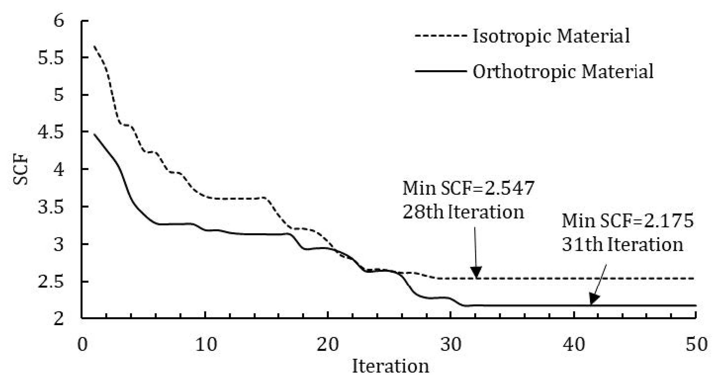
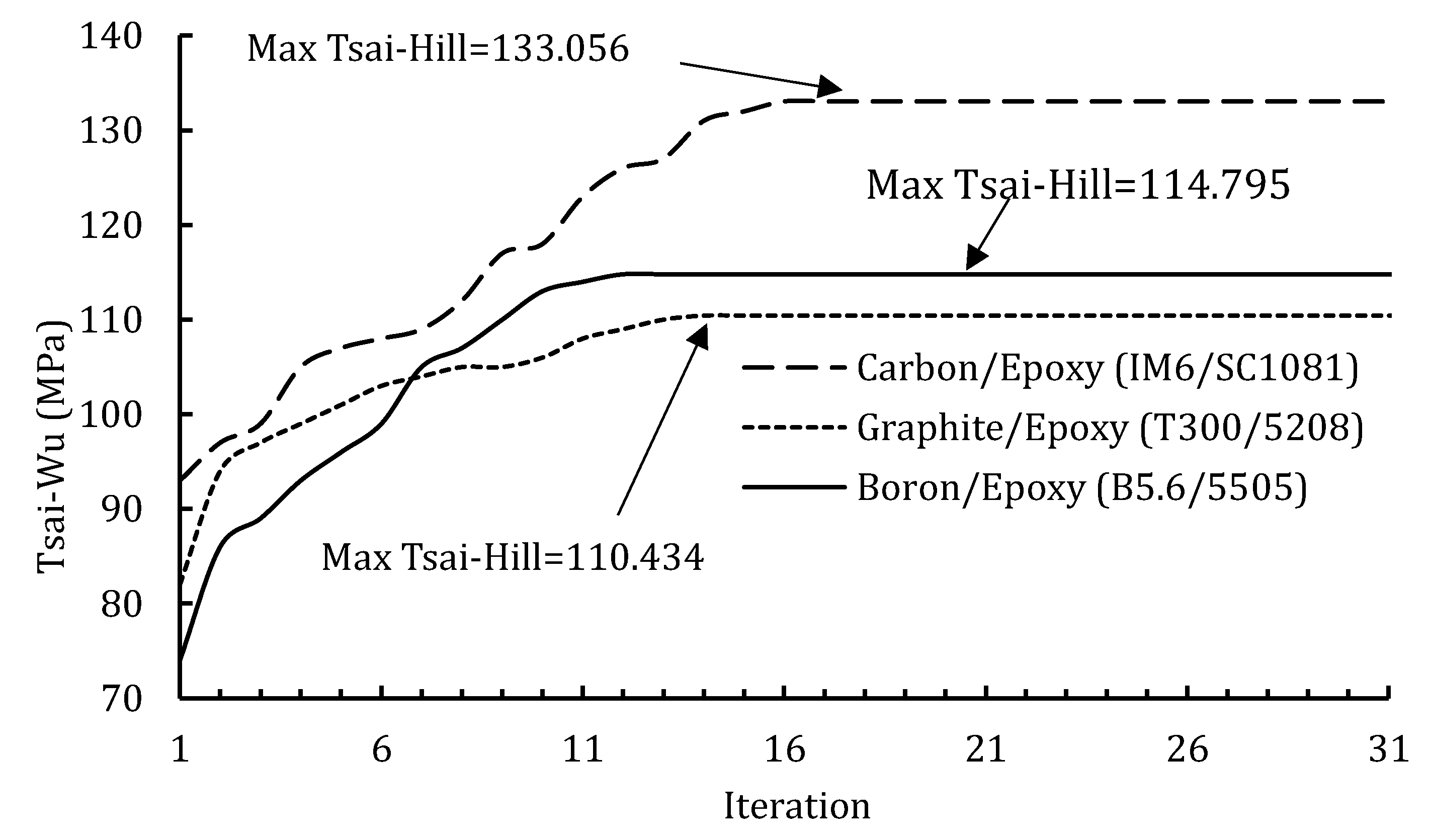
The convergence diagrams for the SCF and fracture criterion (Tsai–Wu) with quasi-square cutout ( c = 1 ) and in the case of uniaxial loading are shown in Figure 6 and Figure 7, respectively.

6. Solution Verification

To examine results obtained from the present analytical method, FEM (ABAQUS software) was employed. For this purpose, firstly, using PSO program code, optimum parameters with quasi-square cutout were determined. Then, the cutout geometry was modeled in accordance with optimum parameters obtained from program execution in ABAQUS software. To achieve optimum mesh number and increased accuracy in the results obtained from finite element numerical solution, meshing was finer around the cutout than external boundaries of the plate.
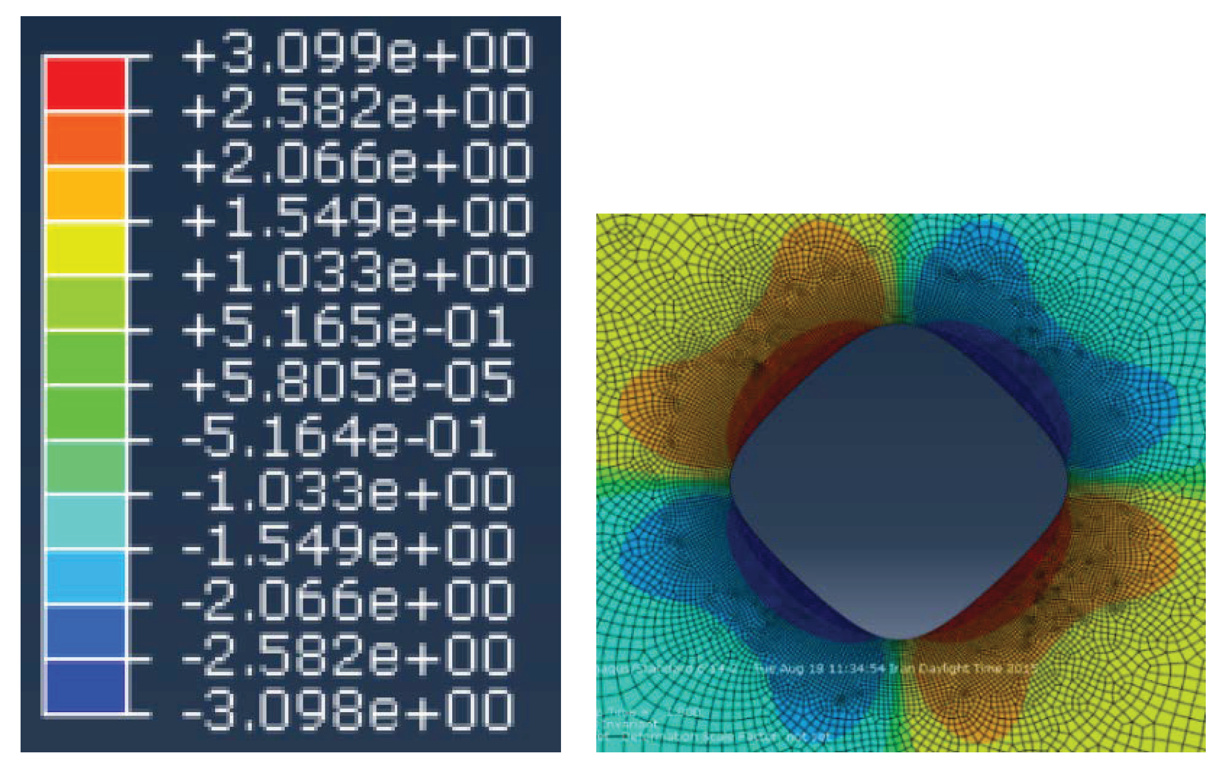
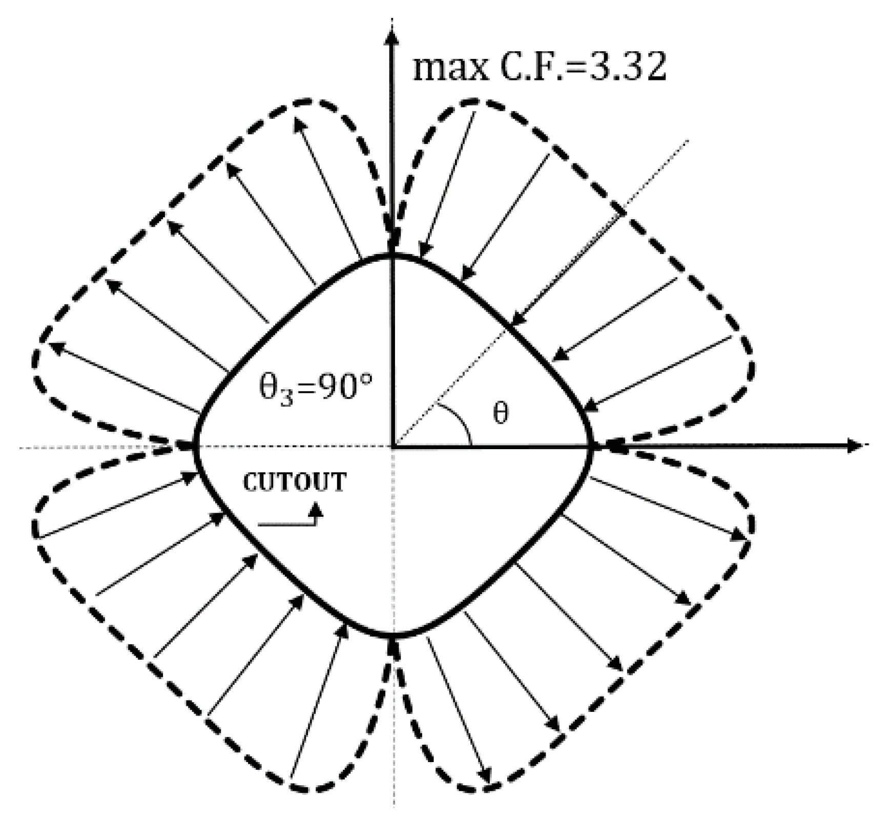
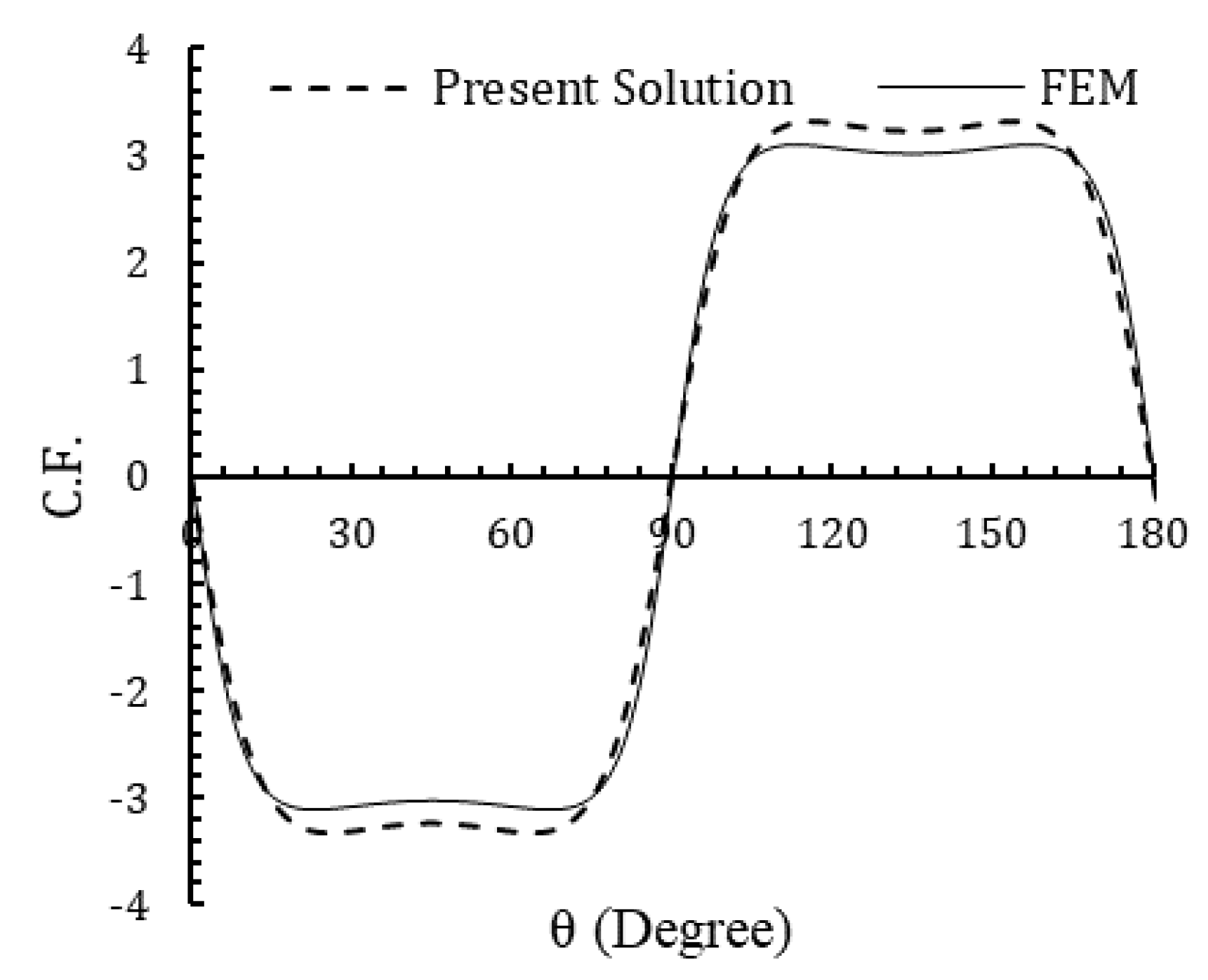
According to this, in an isotropic plate under shear loading, Figure 8 and Figure 9 show the optimum stress distribution modeled in ABAQUS and MATLAB, respectively ( θ 3 = 90 ° , w = 0.078 ). The values obtained from analytical solutions and FEM are compared in Figure 10. Angle θ indicates the points on the boundary cutout relative to the horizontal axis. In isotropic plates, because of the symmetry of stress distribution around the cutout, results to θ = 180 ° are provided. Good agreements between the results obtained by the present solution and FEM show the accuracy and precision of the present analytical solution.
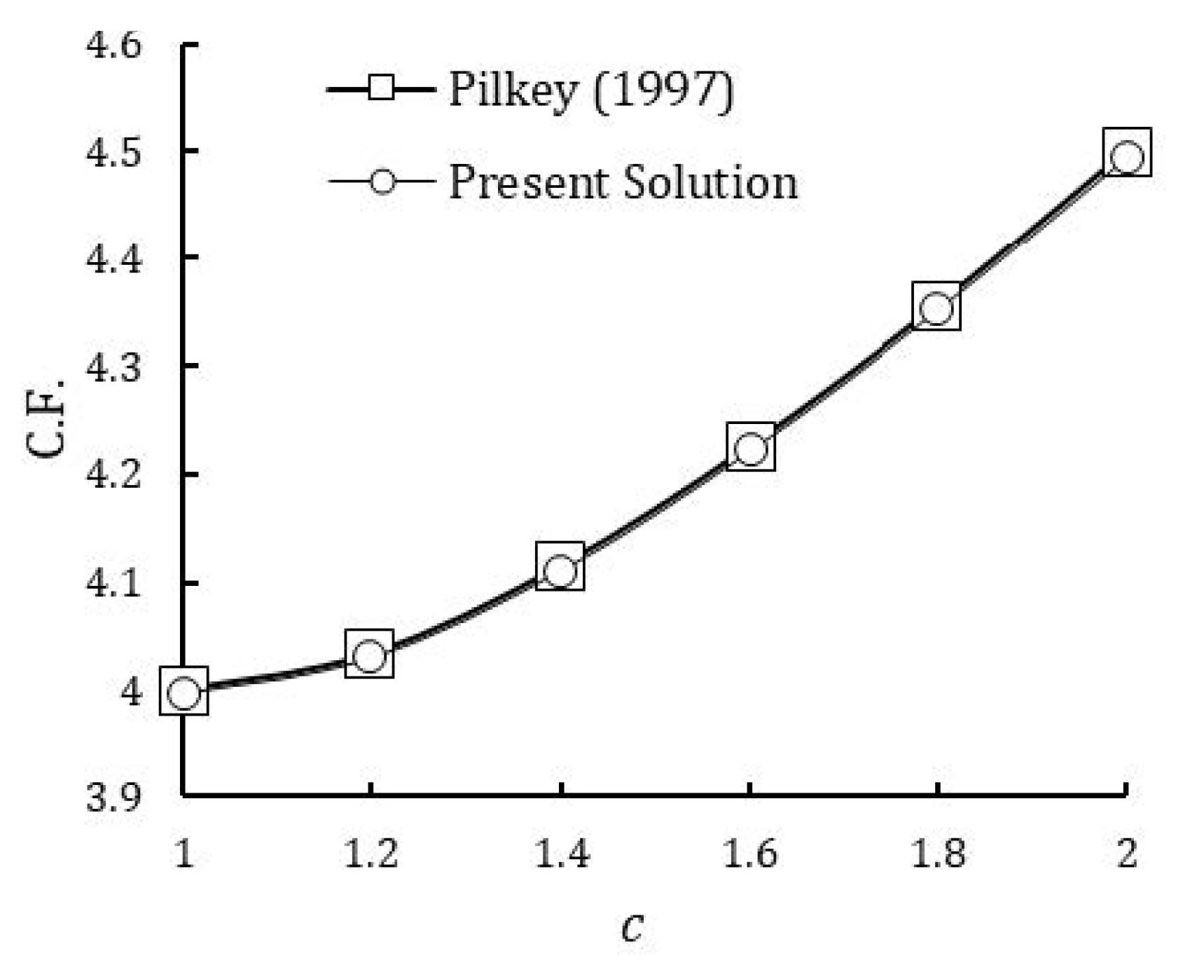
Comparison of the present results in a special case ( θ 3 = 0 ° ) and for shear loading with Pilkeys’ results [72] for an elliptical cutout in the isotropic plate is shown in Figure 11. As shown in this figure, the investigation was conducted based on changing the aspect ratio of cutout. The conformity of results obtained from the two methods indicates the accuracy of the present analytical solution.
For orthotropic plate containing an elliptical cutout with aspect ratio c = 2 , the amount of failure strength based on the Tsai–Wu failure criterion was compared with the results obtained by Ukadgaonker and Rao [73]. For this case, fiber and rotation angles were considered 60 ° and 0 ° , respectively, and the perforated plate was subjected to biaxial tensile. Table 2 shows the conformity of the present solution method with Ukadgaonker and Rao [73].

7. Results and Discussions

Mechanical properties of the used materials are given in Table 3. The normalized stress and the Tsai–Wu criterion are considered as a cost function for the PSO algorithm.

7.1. Isotropic Plates

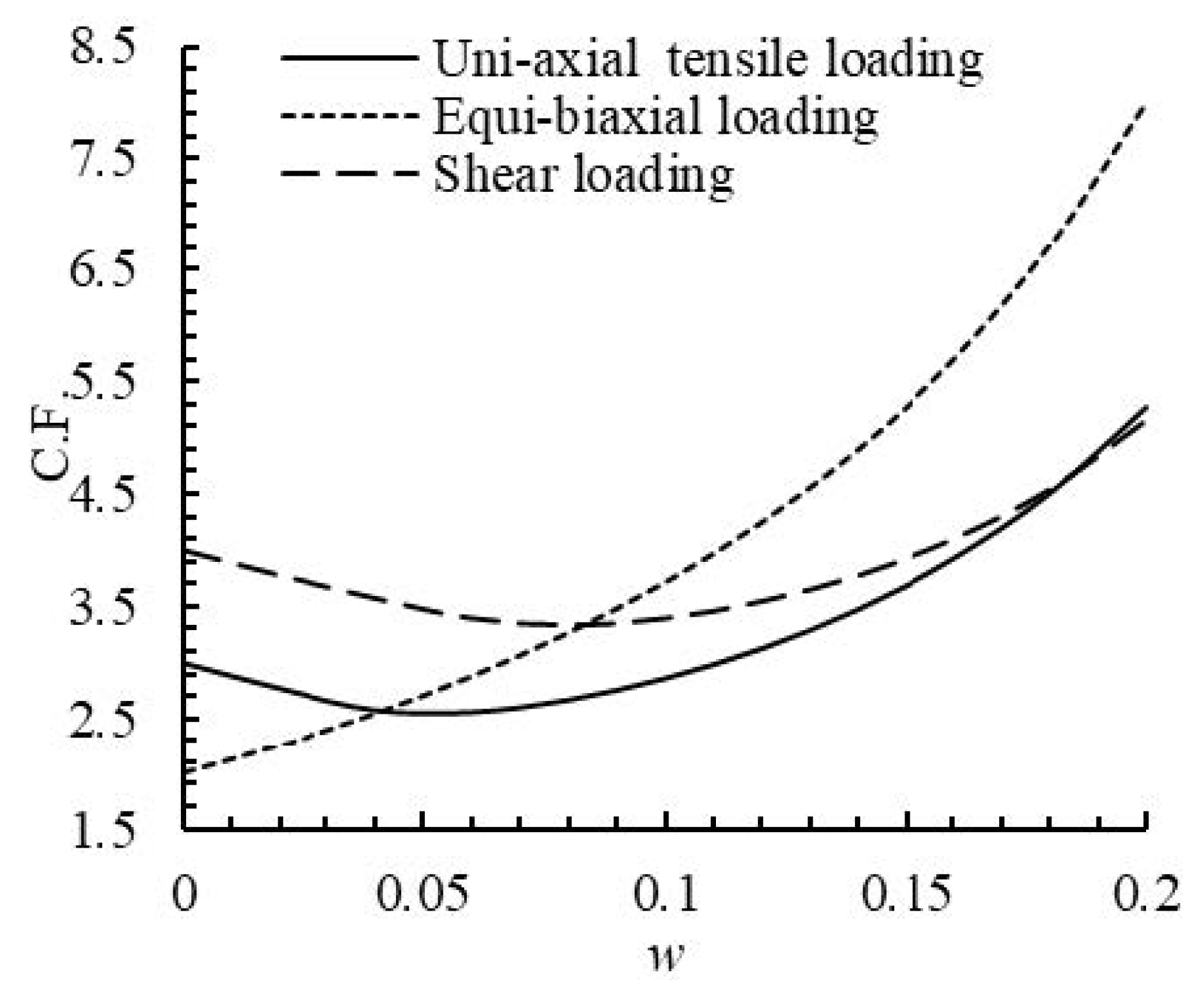
For isotropic plate with quasi-square cutout, a variation of optimal SCF with bluntness parameters for different in-plane loadings is shown in Figure 12. According to this figure, the results of uniaxial and biaxial loadings are different from the shear loading. For biaxial loading, by increasing the value of w, the C.F. rises and minimum C.F. occurs at w = 0 . For uniaxial and shear loadings, minimum C.F. happens at w = 0.052 and w = 0.078 , respectively. w = 0 indicates a circular cutout. In other words, for an isotropic plate with quasi-square cutout and under uniaxial and shear loadings with w = 0.052 and w = 0.078 , respectively, minimum SCF will be less than SCF related to a circular cutout. By changing the value of c, the aspect ratio of the cutout can be controlled. According to Equations (12) and (13), because the aspect ratio parameter ( c ) is in the y-direction of the mapping function, the shape of the cutout is stretched in the y-direction. To study the effect of c, the value of c is considered between 1 and 2 ( 1 < c < 2 ).
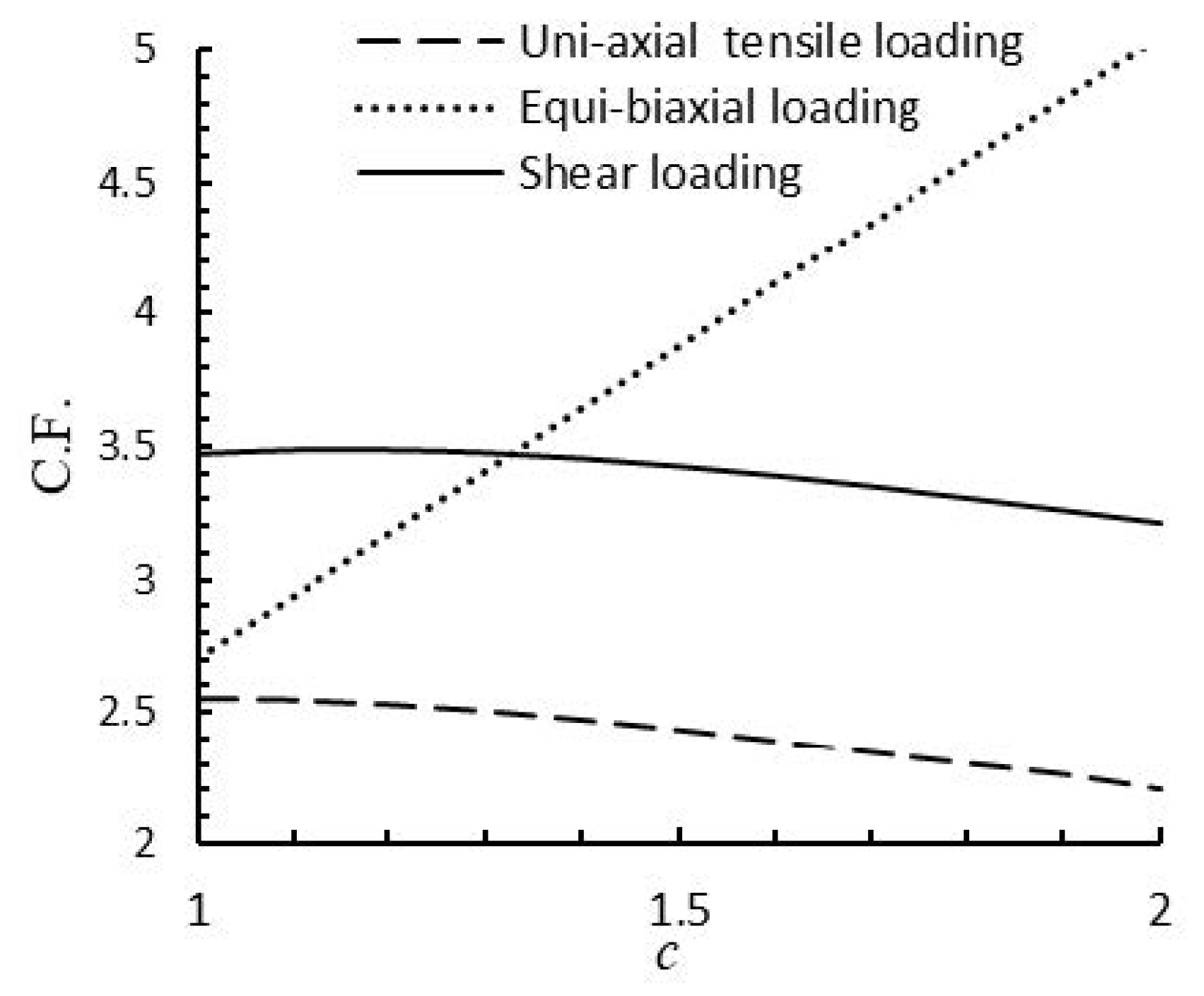
Figure 13 shows the effect of aspect ratio ( c ) for various in-plane loadings on C.F. in optimal values of load angle and rotation angle and w = 0.05 .
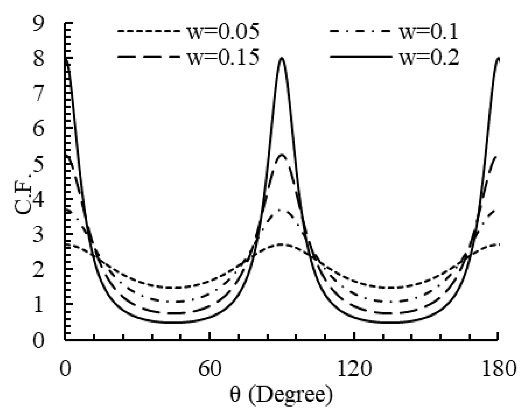
According to this figure, the C.F. varies linearly with c. Except for equibiaxial loading, with increasing value of c, C.F. is reduced. The values of the cost function in an optimal state for circular and elliptical cutout ( w = 0 ) are shown in Table 4 and for rectangular cutout in different values of w are shown in Table 5. Figure 14 shows the change of normalized von Mises stress (cost function) around cutouts in an optimal condition for the isotropic plate.
Table 6 shows the results of the cost function and one of the optimal modes for quasi-square cutout when all effective parameters such as rotation angle, load angle, and bluntness are considered as design variables. The last column of this table represents the percent difference between the optimal C.F. of quasi-square cutout and the corresponding value related to a circular cutout (P.D.).
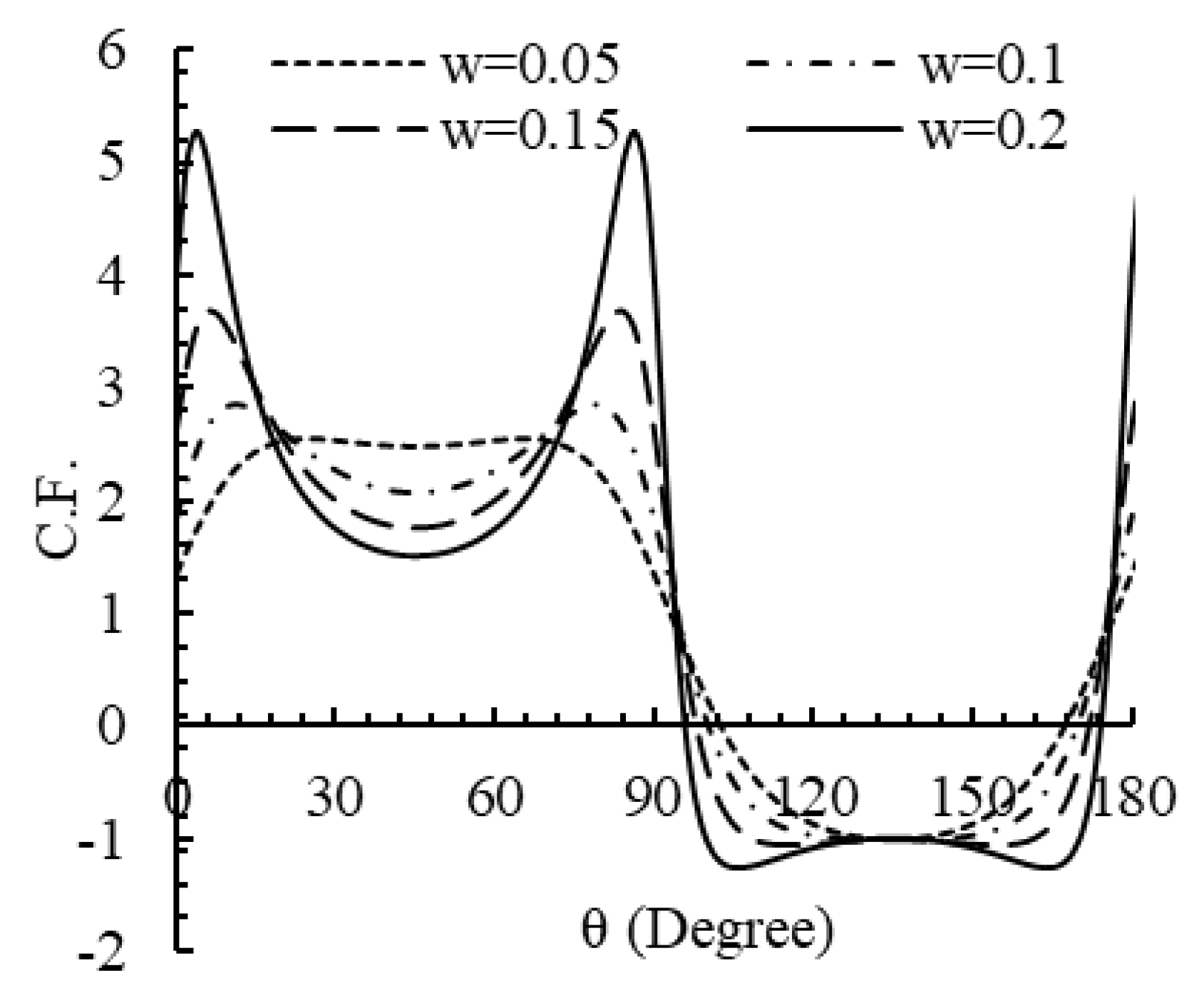
Stress distribution around square cutout in an optimal condition in different values of w and for uniaxial and biaxial tensile loading is shown in Figure 15 and Figure 16.

7.2. Orthotropic Plates

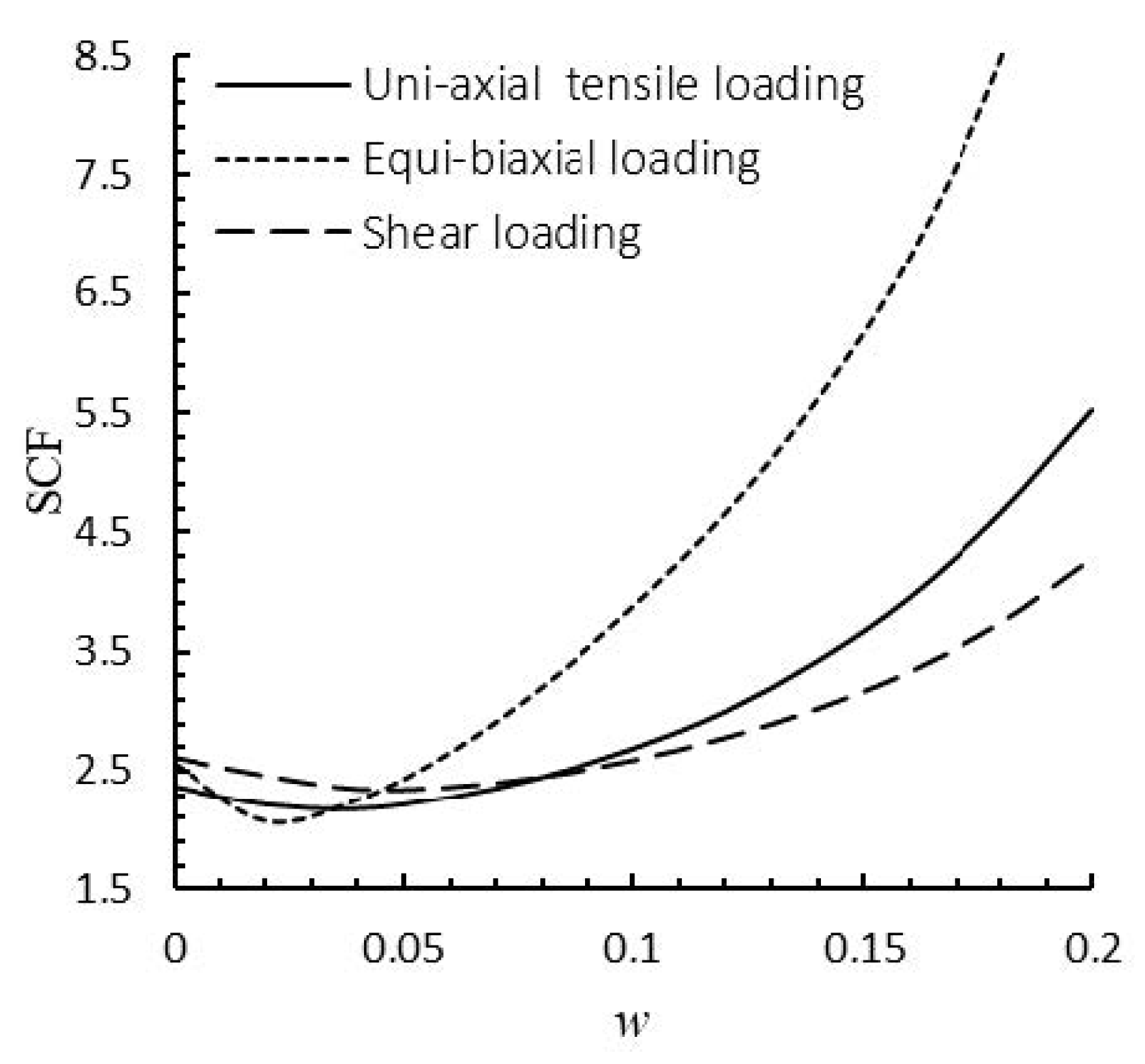
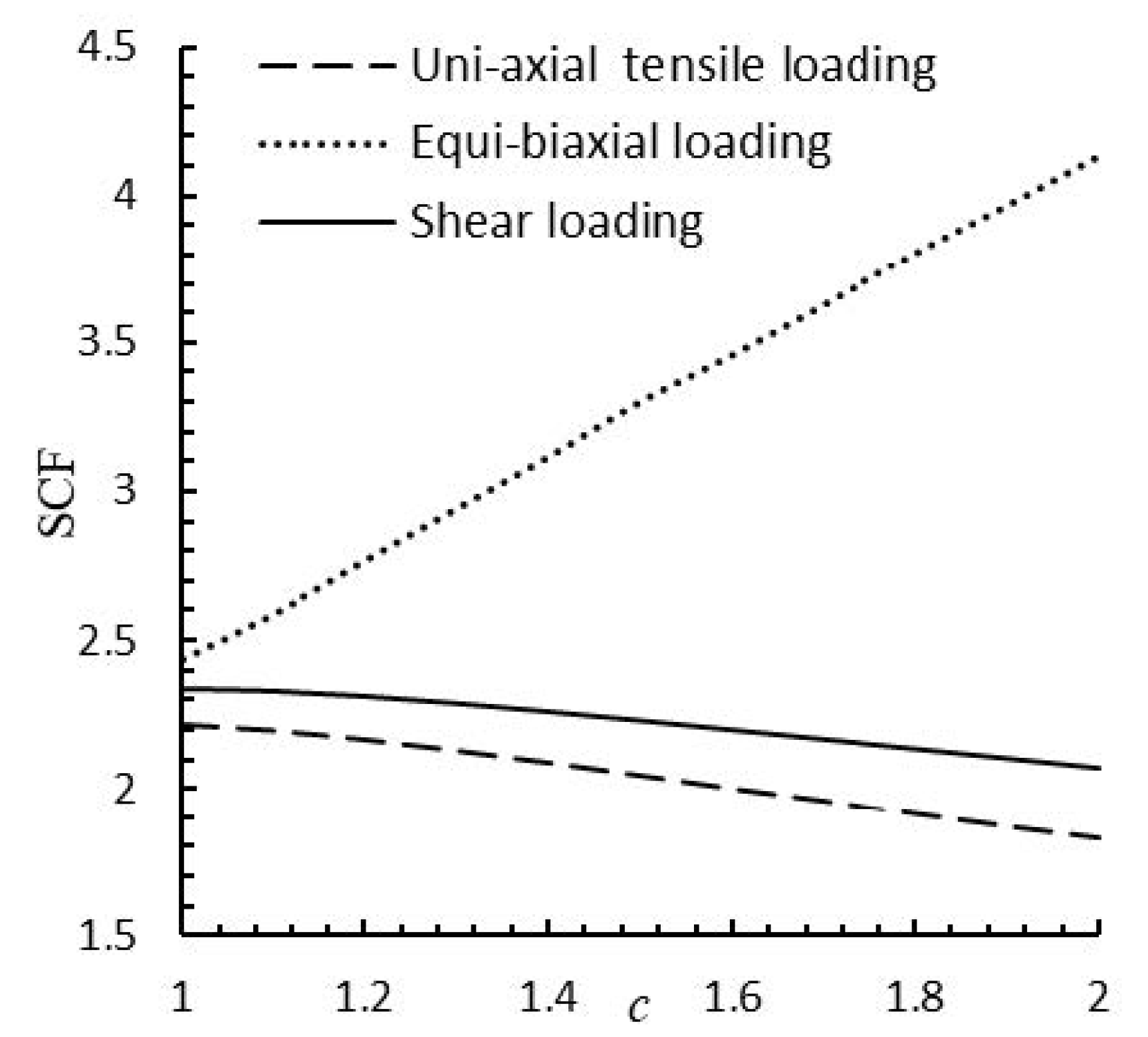
For orthotropic material, the ratio of the maximum stress created around the cutout to applied stress is called a SCF. Variation of SCF for Graphite/Epoxy (T300/5208) plate with quasi-square cutout under different in-plane loadings with bluntness parameter ( w ) is illustrated in Figure 17. According to this figure, the minimum values of C.F. for all three types of loadings occurs in non-zero values for w. Minimum C.F. happens at w = 0.035 , w = 0.020 , and w = 0.045 for uniaxial, biaxial, and shear loadings, respectively. w = 0 is equivalent to a circular cutout. This means square cutout leads to less SCF than circular cutout. Figure 18 shows the effect of aspect ratio of cutout at different types of loadings on SCF. In this case, for w = 0.05 , the optimal results have been achieved for optimal values of load angle, fiber angle, and rotation angle. According to this figure, there is nearly a linear relation between SCF and c.
The values of the cost function in an optimal mode for circular, elliptical cutouts in different values of c and for rectangular cutout for different values of bluntness parameters w are tabulated in Table 7 and Table 8, respectively. Figure 19 shows the stress distribution around quasi-square and elliptical cutouts for graphite/epoxy plate in an optimal condition.
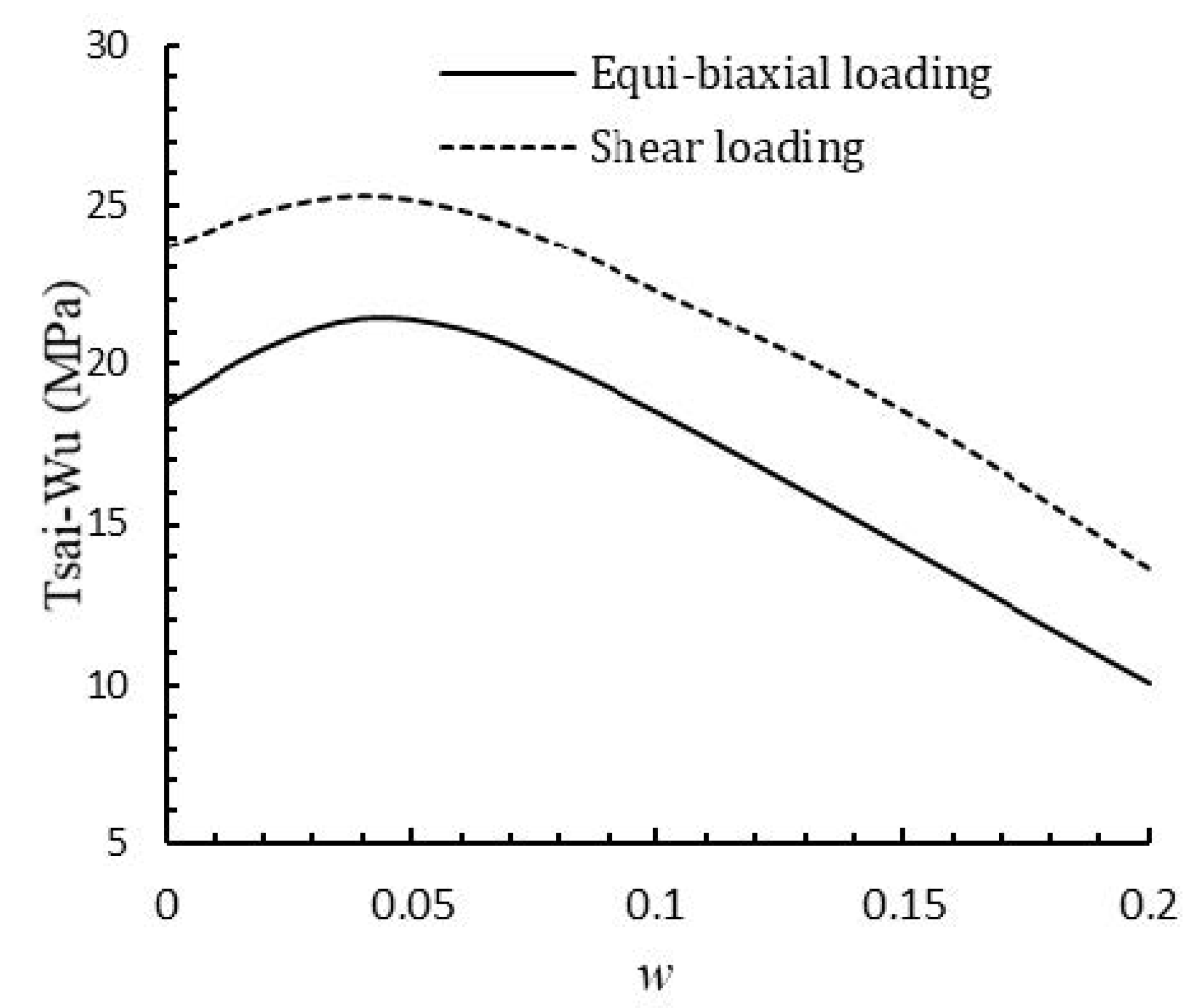
Figure 20 and Figure 21 show the variations of cost function obtained based on Tsai–Wu failure criterion with the bluntness parameter w. The results of Figure 20 are for a square cutout ( c = 1 ) and biaxial and shear loadings, whereas Figure 21 shows strength variations of the graphite/epoxy with w in different values of c; unexpectedly, the optimal value of w is not zero. This means that, by selecting the appropriate values of bluntness parameter, the strength of graphite/epoxy plate with rectangular cutout based on the Tsai–Wu criterion is more than those of a circular cutout. For different values of bluntness ( w ) and aspect ratio of cutout ( c ) , the optimal values of the effective parameters are listed in Table 9. In addition, similar results are presented in Table 10 for triangular cutout. For all values of w, strength increases with increasing c. In this paper, we try to present the results of a square cutout in more detail while the other cutouts only the final results are presented.
Table 11 gives the optimal values of all design variables for quasi-square ( c = 1 ) cutout to achieve the greatest fracture strength. As shown in this table, the maximum value of Tsai–Wu strength occurs at w 0 . P.D. in this table refers to the percent difference between the optimal C.F. of rectangular cutout and the corresponding value related to a circular cutout.
Finally, the optimal values of the design variables for other cutouts are listed in Table 12. As shown in this table, for cutout with an odd number of sides, the highest strength for all in-plane loads occurs at w = 0 . This behavior is not always seen for cutout with an even number of sides.
For perforated composite plates made of different materials, the optimal values of all design variables ( c = 1 ) are listed in Table 13. The results are provided using PSO algorithm. The perforated plate is subjected to uniaxial loading. The results show that for all materials, the optimal values of bluntness parameter w are not zero. Namely, for the case of c = 1 , square cutout with a certain value of w leads to higher failure strength than a circular cutout. The percent difference between failure strength of plate with the square cutout and circular cutout is shown in this table. Optimal cost function (Tsai–Wu strength) is highly dependent on the mechanical properties of the materials. The highest percentage difference is related to Boron/Epoxy and the lowest is related to E-glass/Epoxy. The value of bluntness parameters w is different for various materials.

8. Conclusions

In this study, the PSO algorithm was used to determine the optimal values of effective parameters on stress distribution around different cutouts in orthotropic/iso-tropic infinite plates under in-plane loading. The failure strength obtained from Tsai–Wu criterion was considered as cost function of the PSO algorithm. The analytical solution based on Lekhnitskii method was used to calculate the stress components around the cutout. The results show that the bluntness (w) and aspect ratio of cutout (c) and fiber angle ( θ 2 ), load angle ( θ 1 ), and the cutout orientation ( θ 3 ) have significant effects in reducing the amount of the cost function and by appropriate selection of these parameters the higher failure strength can be achieved. In addition, the effect of material properties of perforated plates on the values of optimal design variables was studied. Optimal values of design variables depend strongly on the mechanical properties of the perforated plate.

Author Contributions

Computing and writing, M.J. and S.A.M.H., writing, literature survey, editing and proofreading, H.A. and E.-M.C. All authors have read and agreed to the published version of the manuscript.

Funding

This research received no external funding.

Conflicts of Interest

The authors declare no conflicts of interest.

References

  1. Dhiraj, V.S.; Jadvani, N.; Kalita, K. Stress and strain analysis of functionally graded plates with circular cutout. Adv. Mater. Res. 2016, 5, 81–92. [Google Scholar] [CrossRef]
  2. Choudhary, P.K.; Jana, P. Position optimization of circular/elliptical cutout within an orthotropic rectangular plate for maximum buckling load. Steel Compos. Struct. 2018, 29, 39–51. [Google Scholar]
  3. Rajanna, T.; Banerjee, S.; Desai, Y.M.; Prabhakara, D.L. Vibration and buckling analyses of laminated panels with and without cutouts under compressive and tensile edge loads. Steel Compos. Struct. 2016, 21, 37–55. [Google Scholar] [CrossRef]
  4. Yang, J.F.; Yang, C.; Su, M.Z.; Lian, M. Stress Concentration factors test of reinforced concrete-filled tubular Y-joints under in-plane bending. Steel Compos. Struct. 2016, 22, 203–216. [Google Scholar] [CrossRef]
  5. Kennedy, J.; Eberhart, R. Particle swarm optimization. In Proceedings of the ICNN’95—International Conference on Neural Networks, Perth, Australia, 27 November–1 December 1995; Volume 4, pp. 1942–1948. [Google Scholar]
  6. Savin, G.N. Stress Distrioution Around Holes; NASA: Washington, DC, USA, 1970.
  7. Green, A.E.; Zerna, W. Theoretical Elasticity, 2nd ed.; Claredon Press: Oxford, UK, 1968. [Google Scholar]
  8. Muskhelishvili, N.I. Some Basic Problems of Mathematical Theory of Elasticity, 2nd ed.; Noordhoff: Leyden, The Netherlands, 1975. [Google Scholar]
  9. Lekhniskii, S.G. Theory of Elasticity of an Anisotropic Body; Holden-Day: San Francisco, CA, USA, 1963. [Google Scholar]
  10. Sih, G.C.; Paris, P.C.; Irwin, G.R. On cracks in rectilinearly anisotropic bodies. Int. J. Fract. Mech. 1965, 1, 189–203. [Google Scholar] [CrossRef]
  11. Lekhniskii, S.G. Theory of Elasticity of an Anisotropic Body; Mir: Moscow, Russia, 1981. [Google Scholar]
  12. Bigoni, D.; Movchan, A. Statics and dynamics of structural interfaces in elasticity. Int. J. Solids Struct. 2002, 39, 4843–4865. [Google Scholar] [CrossRef] [Green Version]
  13. Radi, E.; Bigoni, D.; Capuani, D. Effects of pre-stress on crack-tip fields in elastic, incompressible solids. Int. J. Solids Struct. 2002, 39, 3971–3996. [Google Scholar] [CrossRef]
  14. Craciun, E.M.; Soós, E. Anti-plane States in an Anisotropic Elastic Body Containing an Elliptical Hole. Math. Mech. Solids 2006, 11, 459–466. [Google Scholar] [CrossRef]
  15. Craciun, E.M.; Barbu, L. Compact closed form solution of the incremental plane states in a pre-stressed elastic composite with an elliptical hole. ZAMM J. Appl. Math. Mech./Z. Angew. Math. Mech. 2015, 95, 193–199. [Google Scholar] [CrossRef]
  16. Chaleshtari, M.H.B.; Jafari, M. Optimization of finite plates with polygonal cutout under in-plane loading by gray wolf optimizer. J. Strain Anal. Eng. Des. 2017, 52, 365–379. [Google Scholar] [CrossRef]
  17. Tsutsumi, T.; Sato, K.; Hirashima, K.I.; Arai, H. Stress fields on an isotropic semi-infinite plane with a circular hole subjected to arbitrary loads using the constraint-release technique. Steel Compos. Struct. 2002, 2, 237–246. [Google Scholar] [CrossRef]
  18. Rezaeepazhand, J.; Jafari, M. Stress analysis of perforated composite plates. Compos. Struct. 2005, 71, 463–468. [Google Scholar] [CrossRef]
  19. Yang, Y.; Liu, J.; Cai, C. Analytical solutions to stress concentration problem in plates containing rectangular hole under biaxial tensions. Acta Mech. Solida Sin. 2008, 21, 411–419. [Google Scholar] [CrossRef]
  20. Rao, D.K.N.; Babu, M.R.; Reddy, K.R.N.; Sunil, D. Stress around square and rectangular cutouts in symmetric laminates. Compos. Struct. 2010, 92, 2845–2859. [Google Scholar]
  21. Sharma, D.S. Stress distribution around polygonal holes. Int. J. Mech. Sci. 2012, 65, 115–124. [Google Scholar] [CrossRef]
  22. Banerjee, M.; Jain, N.K.; Sanyal, S. Stress Concentration in Isotropic & Orthotropic Composite Plates with Center Circular Hole Subjected to Transverse Static Loading. Int. J. Mech. Ind. Eng. 2013, 3, 109–113. [Google Scholar]
  23. Marin, M.; Öchsner, A.; Taus, D. On structural stability for an elastic body with voids having dipolar structure. Contin. Mech. Thermodyn. 2019. [Google Scholar] [CrossRef]
  24. Savruk, M.P. Two-Dimensional Problems of Elasticity for Bodies with Cracks; Naukova Dumka: Kiev, Ukraine, 1981. (In Russian) [Google Scholar]
  25. Kazberuk, A.; Savruk, M.P.; Chornenkyi, A.B. Stress distribution at sharp and rounded V-notches in quasi-orthotropic plane. Int. J. Solids Struct. 2016, 85–86, 134–143. [Google Scholar] [CrossRef]
  26. Vigdergauz, S.B. On a case of the inverse problem of two-dimensional theory op elasticity. J. Appl. Math. Mech. 1977, 41, 927–933. [Google Scholar] [CrossRef]
  27. Vigdergauz, S. Three-dimensional grained composites of extreme thermal properties. J. Mech. Phys. Solids 1994, 42, 729–740. [Google Scholar] [CrossRef]
  28. Vigdergauz, S. Two-Dimensional Grained Composites of Extreme Rigidity. J. Appl. Mech. 1994, 61, 390–394. [Google Scholar] [CrossRef]
  29. Grabovsky, Y.; Kohn, R.V. Microstructures minimizing the energy of a two phase elastic composite in two space dimensions. I: The confocal ellipse construction. J. Mech. Phys. Solids 1995, 43, 933–947. [Google Scholar] [CrossRef]
  30. Grabovsky, Y.; Kohn, R.V. Microstructures minimizing the energy of a two phase elastic composite in two space dimensions. II: The vigdergauz microstructure. J. Mech. Phys. Solids 1995, 43, 949–972. [Google Scholar] [CrossRef] [Green Version]
  31. Vigdergauz, S. Rhombic lattice of equi-stress inclusions in an elastic plate. Q. J. Mech. Appl. Math. 1996, 49, 565–580. [Google Scholar] [CrossRef]
  32. Vigdergauz, S. Two-dimensional grained composites of minimum stress concentration. Int. J. Solids Struct. 1997, 34, 661–672. [Google Scholar] [CrossRef]
  33. Vigdergauz, S. Energy-minimizing inclusions in a planar elastic structure with macroisotropy. Struct. Optim. 1999, 17, 104–112. [Google Scholar] [CrossRef]
  34. Cherepanov, G.P. Inverse problems of the plane theory of elasticity. J. Appl. Math. Mech. 1974, 38, 915–931. [Google Scholar] [CrossRef]
  35. Banichuk, N.V. Optimality conditions in the problem of seeking the hole shapes in elastic bodies. J. Appl. Math. Mech. 1977, 41, 946–951. [Google Scholar] [CrossRef]
  36. Banichuk, N.V.; Karihaloo, B.L. On the solution of optimization problems with singularities. Int. J. Solids Struct. 1977, 13, 725–733. [Google Scholar] [CrossRef]
  37. Banichuk, N.V.; Bel’skii, V.G.; Kobelev, V.V. Optimization in problems of the theory of elasticity, with unknown boundaries. Mekhan. Tverd. Tela Izv. Akad. Nauk. 1984, 3, 46–52. [Google Scholar]
  38. Vigdergauz, S.B.; Cherkayev, A.V. A hole in a plate, optimal for its biaxial extension–compression. J. Appl. Math. Mech. 1986, 50, 401–404. [Google Scholar] [CrossRef]
  39. Markenscoff, X. On the Shape of the Eshelby Inclusions. J. Elast. 1997, 49, 163–166. [Google Scholar] [CrossRef]
  40. Cherkaev, A.V.; Grabovsky, Y.; Movchan, A.B.; Serkov, S.K. The cavity of the optimal shape under the shear stresses. Int. J. Solids Struct. 1998, 35, 4391–4410. [Google Scholar] [CrossRef]
  41. Cherepanov, G.P. Mechanics of Brittle Fracture; McGraw-Hill International Book Co.: New York, NY, USA, 1979. [Google Scholar]
  42. Sivakumar, K.; Iyengar, N.G.R.; Deb, K. Optimum design of laminated composite plates with cutouts using a genetic algorithm. Compos. Struct. 1998, 42, 265–279. [Google Scholar] [CrossRef]
  43. Paul, R.J.; Chanev, T.S. Simulation optimisation using a genetic algorithm. Simul. Pract. Theory 1998, 6, 601–611. [Google Scholar] [CrossRef]
  44. Cho, H.; Rowlands, R. Reducing tensile stress concentration in perforated hybrid laminate by genetic algorithm. Compos. Sci. Technol. 2007, 67, 2877–2883. [Google Scholar] [CrossRef]
  45. Chen, J.; Tang, Y.; Ge, R.; An, Q.; Guo, X. Reliability design optimization of composite structures based on PSO together with FEA. Chin. J. Aeronaut. 2013, 26, 343–349. [Google Scholar] [CrossRef] [Green Version]
  46. Zhu, X.; He, R.; Lu, X.; Ling, X.; Zhu, L.; Liu, B. A optimization technique for the composite strut using genetic algorithms. Mater. Des. 2015, 65, 482–488. [Google Scholar] [CrossRef]
  47. Tsai, S.W.; Wu, E.M. A General Theory of Strength for Anisotropic Materials. J. Compos. Mater. 1971, 5, 58–80. [Google Scholar] [CrossRef]
  48. Artar, M.; Daloğlu, A.T. Optimum design of composite steel frames with semi-rigid connections and column bases via genetic algorithm. Steel Compos. Struct. 2015, 19, 1035–1053. [Google Scholar] [CrossRef]
  49. Moussavian, H.; Jafari, M. Optimum design of laminated composite plates containing a quasi-square cutout. Struct. Multidiscip. Optim. 2017, 55, 141–154. [Google Scholar] [CrossRef]
  50. Colorni, A.; Dorigo, M.; Maniezzo, V. Distributed Optimization by Ant Colonies. In Proceedings of the European Conference on Artificial Life, ECAL’91, Paris, France, 11–13 December 1991; Varela, F., Bourgine, P., Eds.; Elsevier: Amsterdam, The Netherlands, 1991; pp. 134–142. [Google Scholar]
  51. Jafari, M.; Rohani, A. Optimization of perforated composite plates under tensile stress using genetic algorithm. J. Compos. Mater. 2016, 50, 2773–2781. [Google Scholar] [CrossRef]
  52. Jafari, M.; Hoseyni, S.A.M. Optimization of infinite orthotropic plates with hypotrochoid cutout under tensile loading using genetic algorithm. J. Reinf. Plast. Compos. 2017, 36, 360–376. [Google Scholar] [CrossRef]
  53. Vosoughi, A.R.; Gerist, S. New hybrid FE-PSO-CGAs sensitivity base technique for damage detection of laminated composite beams. Compos. Struct. 2014, 118, 68–73. [Google Scholar] [CrossRef]
  54. Manjunath, K.; Rangaswamy, T. Ply stacking sequence optimization of composite driveshaft using particle swarm optimization algorithm. Int. J. Simul. Multisci. Des. Optim. 2014, 5, A16. [Google Scholar] [CrossRef] [Green Version]
  55. Ghashochi Bargh, H.; Sadr, M.H. Stacking sequence optimization of composite plates for maximum fundamental frequency using particle swarm optimization algorithm. Meccanica 2012, 47, 719–730. [Google Scholar] [CrossRef]
  56. Kirkpatrick, S.; Gelatt, C.D.; Vecchi, M.P. Optimization by Simulated Annealing. Science 1983, 220, 671–680. [Google Scholar] [CrossRef]
  57. Geyer, C.J. Markov chain Monte Carlo maximum likelihood. In Computing Science and Statistics, Proceedings of the 23rd Symposium on the Interface, Seattle, WA, USA, 21–24 April 1991; Interface Foundation of North America: Fairfax Station, VA, USA, 1991; pp. 156–163. [Google Scholar]
  58. Martino, L.; Elvira, V.; Luengo, D.; Corander, J.; Louzada, F. Orthogonal parallel MCMC methods for sampling and optimization. Digit. Signal Process. 2016, 58, 64–84. [Google Scholar] [CrossRef] [Green Version]
  59. Jafari, M.; Jafari, M. Thermal stress analysis of orthotropic plate containing a rectangular hole using complex variable method. Eur. J. Mech. A/Solids 2019, 73, 212–223. [Google Scholar] [CrossRef]
  60. Lekhniskii, S.G. Anisotropic Plates, 2nd ed.; Gordon & Breach Science Publishers: New York, NY, USA, 1968. [Google Scholar]
  61. Sadd, M.H. Elasticity: Theory, Applications and Numerics; Academic Press: Boston, MA, USA, 2005. [Google Scholar]
  62. Altenbach, H.; Altenbach, J.; Kissing, W. Mechanics of Composite Structural Elements, 2nd ed.; Springer: Singapore, 2018. [Google Scholar]
  63. Bayat, M.; Bayat, M.; Pakar, I. The analytic solution for parametrically excited oscillators of complex variable in nonlinear dynamic systems under harmonic loading. Steel Compos. Struct. 2014, 17, 123–131. [Google Scholar] [CrossRef]
  64. Rezakazemi, M.; Dashti, A.; Asghari, M.; Shirazian, S. H2-selective mixed matrix membranes modeling using ANFIS, PSO-ANFIS, GA-ANFIS. Int. J. Hydrog. Energy 2017, 42, 15211–15225. [Google Scholar] [CrossRef]
  65. Dashti, A.; Harami, H.R.; Rezakazemi, M.; Shirazian, S. Estimating CH4 and CH2 solubilities in ionic liquids using computational intelligence approaches. J. Mol. Liq. 2018, 271, 661–669. [Google Scholar] [CrossRef]
  66. Yang, X.; Yuan, J.; Yuan, J.; Mao, H. A modified particle swarm optimizer with dynamic adaptation. Appl. Math. Comput. 2007, 189, 1205–1213. [Google Scholar] [CrossRef]
  67. Ratnaweera, A.; Halgamuge, S.K.; Watson, H.C. Self-organizing hierarchical particle swarm optimizer with time-varying acceleration coefficients. IEEE Trans. Evol. Comput. 2004, 8, 240–255. [Google Scholar] [CrossRef]
  68. Cherkaev, A. Variational Methods for Structural Optimization; Springer: New York, NY, USA, 2000. [Google Scholar]
  69. Gol’denblat, I.I.; Kopnov, V.A. Strength of glass-reinforced plastics in the complex stress state. Polym. Mech. 1965, 1, 54–59. [Google Scholar] [CrossRef]
  70. Von Mises, R. Mechanik der plastischen Formänderung von Kristallen. ZAMM J. Appl. Math. Mech./Z. Angew. Math. Mech. 1928, 8, 161–185. [Google Scholar] [CrossRef]
  71. Hill, R. A theory of the yielding and plastic flow of anisotropic metals. Proc. R. Soc. Lond. Ser. A Math. Phys. Sci. 1948, 193, 281–297. [Google Scholar]
  72. Pilkey, W.D.; Pilkey, D.F. Peterson’s Stress Concentration Factors, 3rd ed.; John Wiley & Sons, Inc.: Hoboken, NJ, USA, 2008. [Google Scholar]
  73. Ukadgaonker, V.G.; Rao, D.K.N. A general solution for stresses around holes in symmetric laminates under inplane loading. Compos. Struct. 2000, 49, 339–354. [Google Scholar] [CrossRef]
  74. Daniel, I.; Ishai, O. Engineering Mechanics of Composites; Oxford University Press: New York, NY, USA, 1994. [Google Scholar]
Figure 1. Infinite perforated orthotropic plate subject to biaxial loading ( θ 1 is load angle, θ 2 is fiber angle, and θ 3 is cut out orientation).
Mathematics 08 00569 g001
Figure 2. Convert Cartesian coordinate ( x , y ) to curvilinear coordinate ( ρ , θ ).
Mathematics 08 00569 g002
Figure 3. Mapping a plate containing quasi-square cut out to a plate containing a circular cut out.
Mathematics 08 00569 g003
Figure 4. Effect of w on the shape of quasi-square cutout ( c = 1 ).
Mathematics 08 00569 g004
Figure 5. Effect of c parameter on the shape of circular cutout w = 0 , θ 3 = 90 ° (left), effect of c parameter on the shape of quasi-square cutout w = 0.1 , θ 3 = 90 ° (right).
Mathematics 08 00569 g005
Figure 6. Convergence diagram for optimum values with minimum SCF: isotropic material (Steel: w = 0.052 , θ 1 = 90 ° , and θ 3 = 135 ° ) and orthotropic material (Graphite/Epoxy (T300/5208): w = 0.035 , θ 1 = 0 ° , θ 2 = 90 ° , and θ 3 = 135.5 ° ).
Mathematics 08 00569 g006
Figure 7. Convergence diagram for optimum values according to the maximum values of Tsai-Hill (MPa) criterion. Carbon/Epoxy (IM6/SC1081) ( w = 0.05 , θ 1 = 40.6 ° , θ 2 = 90 ° , θ 3 = 135 ° ), Graphite/Epoxy (T300/5208) ( w = 0.052 , θ 1 = 86.7 ° , θ 2 = 88.4 ° , θ 3 = 39.4 ° ), and Boron/Epoxy (B5.6/5505) ( w = 0.056 , θ 1 = 90 ° , θ 2 = 90 ° , θ 3 = 135 ° ).
Mathematics 08 00569 g007
Figure 8. Stress distribution around quasi-square cut out obtained from FEM ( θ 3 = 90 ° and w = 0.0078 ).
Mathematics 08 00569 g008
Figure 9. Optimal stress distribution around quasi-square cutout computed by MATLAB.
Mathematics 08 00569 g009
Figure 10. Comparison of stress distribution around square cutout obtained by FEM and present solution (isotropic plate).
Mathematics 08 00569 g010
Figure 11. Variation of SCF with aspect ratio of elliptical cut out by different methods for isotropic plate ( θ 3 = 0 ° ).
Mathematics 08 00569 g011
Figure 12. Variations of the C.F. in terms of w in different loading ( c = 1 ).
Mathematics 08 00569 g012
Figure 13. Variations of the C.F. in terms of c for rectangular cutout ( w = 0.05 ).
Mathematics 08 00569 g013
Figure 14. Stress distribution around different cutouts in an optimal condition for isotropic plates: (a) uniaxial tensile loading ( w = 0 , C.F. = 1.998 ), elliptical ( c = 2 , θ 1 = 45 ° , θ 3 = 135 ° ); (b) equibiaxial loading ( w = 0 , C.F. = 3.994 ), elliptical ( c = 2 , θ 3 = 135 ° ); (c) shear loading ( w = 0 , C.F. = 2.998 ), elliptical ( c = 2 , θ 3 = 44.5 ° ); (d) uniaxial tensile loading ( w = 0.05 , C.F. = 2.208 ), rectangular ( c = 2 , θ 1 = 70.13 ° , θ 3 = 0 ° ); and (e) shear loading ( w = 0.05 , C.F. = 3.214 ), rectangular ( c = 2 , θ 3 = 26.9 ° ).
Mathematics 08 00569 g014
Figure 15. Distribution of the cost function around square cutout in an optimal state (uniaxial tensile loading).
Mathematics 08 00569 g015
Figure 16. Distribution of the cost function around square cutout in an optimal state (equibiaxial loading).
Mathematics 08 00569 g016
Figure 17. Variations of the SCF with w for quasi-square cutout ( c = 1 ).
Mathematics 08 00569 g017
Figure 18. Variations of the SCF with c in different types of loadings ( w = 0.05 ).
Mathematics 08 00569 g018
Figure 19. Stress distribution around cutout for graphite/epoxy plates in an optimal condition: (a) uniaxial tensile loading ( w = 0 , C.F. = 1.685 ), elliptical ( c = 2 , θ 1 = 88.6 ° , θ 2 = 0 ° , θ 3 = 178.6 ° ); (b) equibiaxial loading ( w = 0 , C.F. = 3.397 ), elliptical ( c = 2 , θ 2 = 0 ° , θ 3 = 69.3 ° ); (c) shear loading ( w = 0 , C.F. = 1.924 ), elliptical ( c = 2 , θ 2 = 45 ° , θ 3 = 45.3 ° ); (d) uniaxial tensile loading ( w = 0.05 , C.F. = 1.826 ), rectangular ( c = 2 , θ 1 = 77.5 ° , θ 2 = 0 ° , θ 3 = 180 ° ); and (e) shear loading ( w = 0.05 , C.F. = 1.826 ), rectangular ( c = 2 , θ 2 = 43 ° , θ 3 = 26.4 ° ).
Mathematics 08 00569 g019
Figure 20. Strength variations of the graphite/epoxy with w ( c = 1 ).
Mathematics 08 00569 g020
Figure 21. Strength variations of the graphite/epoxy with w in different values of c (Uniaxial tensile loading).
Mathematics 08 00569 g021
Table 1. The value of effective parameter for PSO algorithm.
PSO Parameters
Population Size40
Maximum of Iteration50
Cognitive Component c 1 = ( c 1 , f c 1 , i ) I I max + c 1 , i
Social Component c 2 = ( c 2 , f c 2 , i ) I I max + c 2 , i
Inertia Weight ω = ( ω i ω f ) I I max I + ω f
Table 2. Comparison of Tsai–Wu failure strength (MPa) obtained by present solution (p.s.) as well as those of Ukadgaonker and Rao [73] (U&R).
θ p.s.U&R θ p.s.U&R
032.5532.69535.7335.7
540.6440.61003309133.1
1058.0455810530.75630.8
15185.28185.311028.67628.7
20166.18166.211526.81326.8
25181.79181.812025.1425.1
30198.51198.512523.6423.6
35181.2181.213022.3222.3
40150.93150.913522.3222.3
45123.42123.414020.2320.2
50102.07102.114519.5219.5
5586.0278615019.1219.1
6073.973.915519.10819.1
6564.5564.5016019.6419.6
7057.17757.216520.9320.9
7551.23451.217023.2723.3
8046.34346.31752727
8542.24442.218035.7180
9038.75138.8
Table 3. Material properties of the plate by Daniel and Ishai [74].
F 1 F 2 F 6 E 1 E 2 G 12 ν 12
(MPa)(MPa)(MPa)(MPa)(MPa)(MPa)
Steel---20720779.30.3
Graphite/Epoxy (T300/5208)1500406818110.37.170.28
S-glass/Epoxy12804969438.94.50.27
Woven-glass/Epoxy (7781/5245C)36736797.129.729.75.30.17
E-glass/epoxy10803989398.63.80.28
Carbon/Epoxy (IM6/SC1081)2860498317710.87.60.27
Boron/Epoxy (B5.6/5505)1380566220121.75.40.17
Glass/Epoxy1062317238.68.274.140.26
Table 4. Optimal results for circular/elliptical cutout in isotropic plates.
Optimal Values
Uni-Axial Tensile LoadingEqui-Biaxial LoadingShear Loading
w = 0 , c = b / a θ 1 θ 3 | θ 1 θ 3 | C.F. θ 3 C.F. θ 3 C.F.
1 (circular)45--2.996-2.002-3.995
c = 1.5 (elliptical)45134.5589.552.33145–1352.99644.333.330
c = 2 (elliptical)45135901.99845–1353.99444.52.998
Table 5. Optimal results for rectangular cutout in isotropic plates.
Optimal Values
Uni-Axial Tensile LoadingEqui-Biaxial LoadingShear Loading
w c θ 1 θ 3 | θ 1 θ 3 | C.F. θ 3 C.F. θ 3 C.F.
139.61174.59134.982.54845–1352.7020-90-1803.476
0.051.558.85117.5558.72.42845–1353.877773.429
270.130.0070.132.20845–1355.05226.93.214
161.7716.8144.962.85745–1353.7091803.389
0.11.515.67458.42.56045–1355.13680.53.261
217.82131.32135.52.29345–1355.13615.83.141
138.15173.1134.953.68345–1355.2650-90-1803.928
0.151.547167.5120.53.00545–1357.08179.83.488
239.15106.967.752.56645–1358.89716.353.240
18.653.6455.25645–1357.9890-90-1805.149
0.21.517.4135.33117.933.72345–13510.486784.063
287.617.370.32.98845–13512.98318.233.564
Table 6. All optimal values of design parameters for quasi-square cutout in isotropic plate ( c = 1 ).
All Optimal Values for Minimum SCF
w θ 1 θ 3 | θ 1 θ 3 | C.F.P.D.
Uniaxial tensile loading0.05290135452.54715%
Equibiaxial loading0.00---2.0020.00%
Shear loading0.078-0-90-180-3.32816.7%
Table 7. Optimal values of design variables in different aspect ratios of cutout ( w = 0 ).
Optimal Values
Uni-Axial Tensile LoadingEqui-Biaxial LoadingShear Loading
c θ 1 θ 2 θ 3 | θ 1 θ 3 | SCF θ 2 θ 3 SCF θ 2 θ 3 SCF
1 (circular)900--2.37149-2.5514-2.609
5
1.5 (elliptical)901.5180901.91466.151802.70445.452.152
5
2 (elliptical)88.60178.6901.685069.33.397445.31.924
5
Table 8. The optimal values of design variables in different values of bluntness w and aspect ratio of rectangular cutout c.
Optimal Values
Uni-Axial Tensile LoadingEqui-Biaxial LoadingShear Loading
w c θ 1 θ 2 θ 3 | θ 1 θ 3 | SCF θ 2 θ 3 SCF θ 2 θ 3 SCF
190045452.23284.5129.52.5484502.338
0.051.50901171172.04484.5129.53.2864502.338
277.50180102.51.8261684.74.1264326.42.073
1900135452.6885.2550.253.842451802.586
0.11.586.50149.5632.29576.3143.74.18342.5152.342
2740175.5101.51.9799019.55.18447.1267.872.136
10901351353.63339.884.86.1704503.170
0.151.5090112.5112.52.70432.5107.55.5434873.732.639
285.8156.479.42.19333.81009.66.78641.823.532.309
173.517.59844.55.2163517010.7645904.286
0.21.5229098763.19633.6138.67.85649713.121
2575.885.780.72.477601359.5594864.812.576
Table 9. The optimal values of design variables in different values of bluntness w and aspect ratio of rectangular cutout c.
Optimal Values in Different Bluntness for Rectangular Cutout
Uni-Axial Tensile LoadingEqui-Biaxial LoadingShear Loading
w c θ 1 θ 2 θ 3 T.W. (MPa) θ 2 θ 3 T.W. (MPa) θ 2 θ 3 T.W. (MPa)
148.248.2-96.770261-18.75260-23.6921
01.53231.7126.4135.8846474723.86709018025.8111
290900167.7909027.636990026.3309
140.837.690.65109.8832662121.4362018925.2117
0.051.588.5586.4154.4124.53887110022.763690029.1770
243.842.65121.8150.7597493025.193109028.5282
144.6547.987.396.853577.2122.218.525090022.2486
0.11.537.232100.7118.323441.570.520.813709030.2795
218.614.888.8143.070390107.523.365609029.2944
126.620166.569.2347459014.32789018017.7315
0.151.537.232100.7118.323441.570.520.813790027.4709
27175.3180120.923482.39720.435290027.8044
15454.398.847.8697641910.0770018013.6550
0.21.563.267.817874.414768.74614.018509023.7177
279.883.87.299.68605551.717.214509023.8164
Table 10. The optimal values of design variables in different values of bluntness w and aspect ratio of quasi-triangular cutout c.
Optimal Values in Different Bluntness for Quasi-Triangular Cutout
Uni-Axial Tensile LoadingEqui-Biaxial LoadingShear Loading
w c θ 1 θ 2 θ 3 T.W. (MPa) θ 2 θ 3 T.W. (MPa) θ 2 θ 3 T.W. (MPa)
161.259.6127.788.30269018018.011390022.6820
0.051.518.218.14105.56119.770017.2317.6721.749309024.1125
29090180154.51690025.713612.427.3424.7409
188.3681.58150.4176.22489018016.30529018020.9688
0.11.546.9147.95150.59107.711042.3326.5320.141881.631422.5973
29090180138.6020018023.86847520.2323.2315
158.2761.72112.6165.37739018014.22959018018.8204
0.151.576.6578.1718094.5733194.2518.323090019.9144
266.9567.64164.83124.7309146.6322.180917.1868.4721.5115
146.5050.07101.5053.581990012.04499018016.4227
0.21.554.0755.80156.7482.212522.909.5516.422111.7273.9218.4941
24847.16130.74111.57119084.2420.472470.4423.1719.6876
Table 11. Optimal values of all design variables for square cutout ( c = 1 ).
All Optimal Values
All Optimal Values for minimum SCFAll Optimal Values for maximum Tsai–Wu
w θ 1 θ 2 θ 3 SCFP.D.w θ 1 θ 2 θ 3 T.W. (MPa)P.D.
Uniaxial0.035090135.52.1758%0.05286.788.439.4110.434514%
Equibiaxial0.020-55102.03120%0.045-73.6118.621.494514%
Shear0.045-44.590.52.33610%0.039-90025.34077%
Table 12. All optimal values of design parameters for another cutout ( c = 1 ).
Uni-Axial Tensile LoadingEqui-Biaxial LoadingShear Loading
w θ 1 θ 2 θ 3 T.W. (MPa)w θ 2 θ 3 T.W. (MPa)w θ 2 θ 3 T.W. (MPa)
Pentagonal0.00909018096.39920.0080.518018.75260.009039.523.6940
Hexagonal0.0130.000.0018099.25590.01334419.97640.009015.523.6940
Heptagonal0.009090121.596.47690.009014118.75260.000.0076.523.6940
Octagonal0.009090104.596.47690.0058820.519.45780.0090145.523.6940
Table 13. Optimal values of the design parameters for different materials ( c = 1 ) with respect to Tsai–Wu.
Optimum Failure Strength Subjected to Uniaxial Tensile Loading
Graphite/Epoxy (T300/5208)S-Glass/EpoxyWoven-Glass/EpoxyGraphite/EpoxyCarbon/EpoxyE-Glass/EpoxyBoron/Epoxy (B5.6/5505)
w0.0520.0320.0470.0720.0500.0890.056
θ 1 86.736.668.736.440.629.790
θ 2 88.435.27846.2337.720.790
θ 3 39.4175.318.5155.41800.00135
Optimal110.43491.005107.75567.781133.05684.206114.795
Tsai–Wu
P.D.14%5%10%2.5%13%1.5%19.5%
Tsai–Wu96.77086.54898.07266.105117.96782.85096.110
(circular)