Global Analysis of a Reaction-Diffusion Within-Host Malaria Infection Model with Adaptive Immune Response

Abstract

Malaria is one of the most dangerous global diseases. This paper studies a reaction-diffusion model for the within-host dynamics of malaria infection with both antibody and cell-mediated immune responses. The model explores the interactions between uninfected red blood cells (erythrocytes), three types of infected red blood cells, free merozoites, CTLs and antibodies. It contains some parameters to measure the effect of antimalarial drugs and isoleucine starvation on the blood cycle of malaria infection. The basic properties of the model are discussed. All possible equilibrium points and the threshold conditions required for their existence are addressed. The global stability of all equilibria are proved by selecting suitable Lyapunov functionals and using LaSalle’s invariance principle. The characteristic equations are used to study the local instability conditions of the equilibria. Some numerical simulations are conducted to support the theoretical results. The results indicate that antimalarial drugs with high efficacy can clear the infection and take the system towards the disease-free state. Increasing the efficacy of isoleucine starvation has a similar effect as antimalarial drugs and can eliminate the disease. The presence of immune responses with low efficacy of treatments does not provide a complete protection against the disease. However, the immune responses reduce the concentrations of all types of infected cells and limit the production of malaria parasites.

1. Introduction

Malaria is an infectious diseases caused by Plasmodium parasite. In 2018, about 228 million cases of malaria occurred around the world [1]. Most of these cases were in the World Health Organization (WHO) African Region with $93\%$, followed by the South-East Asia Region with $3.4\%$ and the Eastern Mediterranean Region with $2.1\%$ [1]. The global malaria deaths in 2018 were estimated at 405,000 deaths, where children under age 5 years accounted for $67\%$ of these deaths. In 2018, there were 11 million pregnant women exposed to malaria infections and they delivered about 872,000 children with low birth weight [1]. Plasmodium falciparum (P. falciparum) is the most popular malaria parasite and it is accounted for the highest number of malaria cases [1]. The other four Plasmodium species that infect humans are P. vivax, P. ovale, P. malariae and P. knowlesi [2,3]. The malaria infection within a host is composed of two phases, the liver stage and the blood stage [3]. The blood stage is associated with the clinical symptoms of the infection. The infection begins by the bite of an infected Anopheles mosquito to take a blood meal. During the bite, it releases the malaria parasite in the form of sporozoites into the bloodstream of the host. The sporozoites migrate to the liver where they infect the liver cells and develop into schizonts. After rupturing, the schizonts release the parasites in the form of merozoites into the bloodstream where the blood stage starts [2,4,5]. The merozoites invade red blood cells and develop within them through three morphological stages. The youngest stage is the ring stage which grows into the trophozoite stage, and finally into the schizont stage. The schizont ruptures to produce 8–32 daughter merozoites which invade healthy red blood cells and repeat the infection cycle [3]. The merozoites are the asexual form of the malaria parasite. Nevertheless, some of the merozoites develop into gametocytes which are the sexual form of the parasite [5]. Artemisinin-based combination therapies (ACTs) are the current standard treatment for the blood stage of P. falciparum malaria infection [6,7]. In this paper, we focus on the asexual blood-stage dynamics of P. falciparum.

Mathematical modeling has been used to understand the dynamics of malaria parasites during infection and to design more effective antimalarial drugs. Malaria models were built using similar ideas to those used in virus dynamics models [8,9,10,11,12,13,14,15,16]. The basic model for the within-host dynamics of malaria infection was proposed by Anderson et al. [17]. The model takes the form

$$\left\{\begin{array}{l}\frac{dU\left(t\right)}{dt}=\mu -\tilde{d}U\left(t\right)-\beta U\left(t\right)M\left(t\right),\\ \frac{dY\left(t\right)}{dt}=\beta U\left(t\right)M\left(t\right)-eY\left(t\right),\\ \frac{dM\left(t\right)}{dt}=\eta eY\left(t\right)-fM\left(t\right)-g\beta U\left(t\right)M\left(t\right),\end{array}\right.$$

(1)

where $g=1$. The variables $U\left(t\right)$, $Y\left(t\right)$, and $M\left(t\right)$ denote the concentrations of uninfected red blood cells, infected red blood cells, and free merozoites, respectively. Uninfected red blood cells are recruited from the bone marrow at a constant rate $\mu$, infected by free merozoites at rate $\beta UM$, and die at a natural death rate $\tilde{d}U$. Infected red blood cells die at rate $eY$ and rupture to produce $\eta$ merozoites per infected cell. The total production rate of merozoites is given by $\eta eY$. Free merozoites either die at rate $fM$ or infect red blood cells at rate $\beta UM$ [17]. A similar model was investigated by Anderson [18] but with $g=0$. The models in [17,18] were extended in multiple ways to include other components or processes. In [19], A. Saul argued that the basic models contain an error which leads to overestimation of parasite growth rates. To avoid this error, he suggested using the growth rate constant $e(ln(\eta )+1)$ instead of $e\eta$. However, Gravenor and Lloyd [20] mentioned that Saul’s suggestion does not solve the problem of large growth rates. Alternatively, they proposed a model with n categories for the infected erythrocytes. The transition between these classes is governed by constant rates. Hoshen et al. [21] introduced a delay differential equation model of blood-stage malaria infection. The model contains a parameter $\tau$ to model the lifespan of the infected erythrocytes ($\tau =48$ h in the case of P. falciparum). They converted the nonlinear equations into linear equations and they got the analytic solution by using suitable biological analysis of non-severe malaria. Iggidr et al. [22] performed a global analysis of the model suggested in [20] with a general recruitment rate for the uninfected red blood cells. In addition, they proposed and analyzed a model with n strains and k classes of infected erythrocytes. They identified the conditions under which one strain persists while all other strains die out. Saralamba et al. [23] developed a model to explore parasite population dynamics in age and time. They examined the effect of antimalarial drug on the killing rate of parasites at the three sequential asexual blood stages; rings, trophozoites, and schizonts. They suggested that the drug resistance is concentrated at the ring stage. Demasse and Ducrot [24] extended the model developed in [22] and proposed an age-structured blood-stage malaria model. They showed the global stability of the disease-free equilibrium and the positive equilibrium associated with the strongest strain.

The blood-stage infection stimulates different immune responses to fight the infection and limit the growth of parasites [25]. The adaptive immunity plays a major role in fighting the disease. There are two types of adaptive immunity which are antibody immunity and cellular immunity. Cellular immunity stimulates the production of cytotoxic T lymphocytes (CTLs) to kill infected cells. Antibody immunity is mediated by B cells which produce antibodies to clear free merozoites from the blood [25,26]. It was mentioned that antibody immunity is more effective than cellular immunity [26]. However, this depends on the magnitude of each one of the two immune responses and their ability to constrict parasite replication. For simplicity, many works have added only one component to their models to represent the total capacity of the immune response directed against both infected red blood cells and free merozoites. For example, Anderson et al. [17] added the immune response to model (1) as follows

$$\left\{\begin{array}{l}\frac{dU\left(t\right)}{dt}=\mu -\tilde{d}U\left(t\right)-\beta U\left(t\right)M\left(t\right),\\ \frac{dY\left(t\right)}{dt}=\beta U\left(t\right)M\left(t\right)-eY\left(t\right)-{\tilde{\alpha }}_{1}Y\left(t\right)Z\left(t\right),\\ \frac{dM\left(t\right)}{dt}=\eta eY\left(t\right)-fM\left(t\right)-g\beta U\left(t\right)M\left(t\right)-{\tilde{\alpha }}_{2}M\left(t\right)Z\left(t\right),\\ \frac{dZ\left(t\right)}{dt}={\tilde{\rho }}_{1}Y\left(t\right)Z\left(t\right)+{\tilde{\rho }}_{2}M\left(t\right)Z\left(t\right)-hZ\left(t\right),\end{array}\right.$$

(2)

where $Z\left(t\right)$ denotes the concentration of immune cells. The clearance rates of infected red blood cells and free merozoites by immune cells are given by ${\tilde{\alpha }}_{1}YZ$ and ${\tilde{\alpha }}_{2}MZ$, respectively. The infected red blood cells and free merozoites stimulate the production of immune cells at rates ${\tilde{\rho }}_{1}YZ$ and ${\tilde{\rho }}_{2}MZ$, respectively. The death rate of immune cells is given by $hZ$. The other parameters have the same biological meanings as those in model (1). Hetzel and Anderson [27] studied an extended version of model (1) with an additional equation for an immune response. They performed experiments to estimate the invasion rate of red blood cells. Tumwiine et al. [26] explored an extended version of model (2), where they established the existence and global stability of equilibrium points. Niger and Gumel [4] extended the models in [20] and [22] by adding the effects of immune response and malaria vaccines. They proved the global stability of the parasite-free equilibrium. Li et al. [25] expanded the model studied by Anderson et al. [17] by using nonlinear Michaelis-Menten-Monod functions to describe the proliferation rate of the immune response and the removal rates of both the infected cells and free merozoites by immune effectors. They investigated the existence and local stability of the equilibrium points. They also proved that the model undergoes Hopf bifurcation at the positive equilibrium and shows periodic oscillations, where the proliferation rate of immune cells is taken as a bifurcation parameter. Tewa et al. [28] analyzed a general within-host model of malaria infection with immune response. The production rate of healthy erythrocytes and the stimulation rate of immune response are given by general functions with suitable hypotheses. Tchinda et al. [29] considered a particular form of the model studied in [28]. The dynamics of the immune response is modeled by “Allee effect“, where the immune response cannot persist under certain thresholds. They explored the existence and local stability of model’s equilibria. On the other hand, some works have differentiated between the immune response that targets infected red blood cells, and the immune response that targets free merozoites. For instance, Chen et al. [2] studied a blood-stage malaria infection model with two competitive strains of P. falciparum and two types of immune responses, namely cellular immunity and antibody immunity. The infection rates and the stimulation rates of the immune responses are provided by saturated rates. They identified the global stability conditions of the equilibrium point at which two strains of malaria parasite coexist. Cai et al. [30] proposed within-host models for symptomatically and asymptomatically infected hosts. The infected cells are divided into immature trophozoites and mature trophozoites. The model contains an immune response directed against mature trophozoites. The dynamics of this model was linked to a between-host model. Orwa et al. [31] formulated and analyzed a within-host model for malaria infection with malaria vaccines and CTL immune response. The infected red blood cells are classified into blood trophozoites and schizonts. They showed that the parameter which represents the average number of merozoites released per schizont infected red blood cell is the most sensitive parameter in their model. Song et al. [6] developed and analyzed a model to study the evolution of drug resistance parasites in the presence of a competition with drug sensitive parasites, immune response, and antimalarial drug. The effects of CTL and antibody immune responses on malaria infection are examined in this paper.

The previous works did not take into account the spatial effects, and they assumed that the spatial distribution of cells and merozoites are homogeneous. The homogeneity assumption is unrealistic for many reasons: (i) many parasites during malaria infection accumulate in organs such as the brain and lungs [3]; (ii) there might be local restriction on the availability of uninfected red blood cells, which can reduce their contact with free merozoites [27]; (iii) the interaction between pathogens and the immune response tends to be local within the body of infected hosts [32]; (iv) red blood cells and merozoites are in motion [21]. Hence, more realistic models should take into consideration the non-uniform distribution of cells and merozoites across the body of the host in addition to their ability to move within the body [3,27]. In [33], Takoutsing et al. investigated a reaction-diffusion model for the within-host dynamics of malaria with a periodic antimalarial drug and immune factors. They examined the effect of treatment duration and efficacy on the distribution of parasites in space and time. Another factor that was not considered in the previous models is the perturbation of the blood-stage asexual life-cycle of malaria due to nutrient deprivation [3,34]. The degradation of host erythrocyte hemoglobin releases amino acids which represent a nutrient source for the malaria parasite P. falciparum. Nevertheless, human hemoglobin does not contain the single amino acid isoleucine which exists in more than $99\%$ of the proteins encoded by the parasite [34]. Thus, the parasite must get isoleucine from an extracellular source for its survival. It has been shown that when the concentration of isoleucine is low, the parasite slows its metabolism and progresses from the ring stage to the trophozoite stage at a reduced rate. This helps the parasite to save energy and resources during isoleucine starvation. However, this starvation can protect the parasite for certain periods and the parasite may not be able to recover after long periods of starvation [34]. The spatial effects and the impact of isoleucine starvation on the growth of malaria parasites are considered in this paper.

The aim of this paper is to study a reaction-diffusion model for the within-host dynamics of malaria infection with both CTL and antibody immune responses. The model includes the effects of blood-stage antimalarial drugs and isoleucine starvation on parasite dynamics. Furthermore, the model captures the progression of infected red blood cells through the three developmental stages: ring stage, trophozoite stage, and schizont stage. Therefore, the model is considered to be an extension of the models studied in [23,31], where the effect of isoleucine starvation, spatial factors, or the ring stage are not involved.

2. A Reaction-Diffusion within-Host Malaria Model with both Cytotoxic T Lymphocyte and Antibody Immune Responses

In this section, we provide a complete description of the model under consideration. The proposed model captures the interaction of uninfected red blood cells, infected red blood cells, free blood merozoites, CTLs, and antibodies. In the formulation of the model, we make the following assumptions:

(i)

The dynamics of uninfected red blood cells is similar to the one given in model (1);

(ii)

The infected red blood cell population is divided into ring, trophozoite, and schizont infected red blood cells;

(iii)

The ring infected red blood cells increase due to the invasion of healthy red blood cells, and they decrease due to either the development into trophozoite infected red blood cells or natural death;

(iv)

The trophozoite infected red blood cells decrease due to either the development into schizont infected red blood cells or natural death;

(v)

The schizont infected red blood cells are depleted due to either the CTLs or natural death;

(vi)

Free merozoites in the blood increase as a result of schizonts bursting, and they decrease due to either the removal by antibodies or natural death;

(vii)

CTLs are stimulated by schizont infected red blood cells, while the production of antibodies is stimulated by free merozoites;

(viii)

CTLs and antibodies decrease duo to natural decay rates.

Hence, motivated by [23,31,33], we study the following reaction-diffusion malaria model

$$\left\{\begin{array}{l}\frac{\partial U(x,t)}{\partial t}=D_U\Delta U(x,t)+\mu -\tilde{d}U(x,t)-\beta (1-{\epsilon }_1)U(x,t)M(x,t),\\ \frac{\partial N(x,t)}{\partial t}=D_N\Delta N(x,t)+\beta (1-{\epsilon }_1)U(x,t)M(x,t)-{\gamma }_1(1-b)N(x,t)-d_{1}N(x,t),\\ \frac{\partial T(x,t)}{\partial t}=D_T\Delta T(x,t)+{\gamma }_1(1-b)N(x,t)-{\gamma }_{2}T(x,t)-d_{2}T(x,t),\\ \frac{\partial S(x,t)}{\partial t}=D_S\Delta S(x,t)+{\gamma }_{2}T(x,t)-{\alpha }_{1}S(x,t)W(x,t)-d_{3}S(x,t),\\ \frac{\partial M(x,t)}{\partial t}=D_M\Delta M(x,t)+\eta d_3(1-{\epsilon }_2)S(x,t)-{\alpha }_{2}M(x,t)B(x,t)-d_{4}M(x,t),\\ \frac{\partial W(x,t)}{\partial t}=D_W\Delta W(x,t)+{\rho }_{1}S(x,t)W(x,t)-d_{5}W(x,t),\\ \frac{\partial B(x,t)}{\partial t}=D_B\Delta B(x,t)+{\rho }_{2}M(x,t)B(x,t)-d_{6}B(x,t),\end{array}\right.$$

(3)

for $x\in \Omega$ and $t>0$, where $\Omega$ is a connected and bounded spatial domain with smooth boundary $\partial \Omega$. The variables $U(x,t)$, $N(x,t)$, $T(x,t)$, $S(x,t)$, $M(x,t)$, $W(x,t)$, and $B(x,t)$ denote the concentrations of uninfected red blood cells, ring infected red blood cells, trophozoite infected red blood cells, schizont infected red blood cells, free merozoites, CTLs, and antibodies at position x and time t, respectively. We assume that red blood cells, free merozoites, and immune cells diffuse freely in the domain with different abilities. In the diffusion terms, $D_{\Lambda }$ is the diffusion coefficient of the component $\Lambda$, and $\Delta =\frac{{\partial }^2}{\partial x^2}$ is the Laplacian operator. Ring infected red blood cells develop into trophozoite infected cells at rate ${\gamma }_{1}N$, while trophozoites are developed into schizont infected cells at rate ${\gamma }_{2}T$. CTLs attack and kill schizont infected red blood cells at rate ${\alpha }_{1}SW$, while they are stimulated at rate ${\rho }_{1}SW$. Free merozoites are neutralized by antibodies at rate ${\alpha }_{2}MB$, and antibodies grow at rate ${\rho }_{2}MB$. The death rates of rings, trophozoites, schizonts, free merozoites, CTLs, and antibodies are given by $d_{1}N$, $d_{2}T$, $d_{3}S$, $d_{4}M$, $d_{5}W$, and $d_{6}B$, respectively. The symbols ${\epsilon }_1$ and ${\epsilon }_2$ measure the efficacy of antimalarial drugs that affect the infection rate of healthy cells and the production rate of free merozoites, where $0\le {\epsilon }_1<1$ and $0\le {\epsilon }_2<1$. The symbol b measures the efficacy of isoleucine starvation, where $0\le b<1$. The other parameters have the same biological meanings as those in model (1). The full description of all parameters is given in

Table 1. Parameters values of model (3).

Parameter	Description	Value	Reference
$\mu$	Recruitment rate of red blood cells	$2.5\times {10}^8$ cell mL${}^{-1}$day${}^{-1}$	[27]
$\tilde{d}$	Death rate of uninfected red blood cells	$0.025$ day${}^{-1}$	[27]
$\beta$	Infection rate of red blood cells	Varied	–
${\gamma }_1$	Progression rate from rings to trophozoites	$0.1$ day${}^{-1}$	[31]
${\gamma }_2$	Progression rate from trophozoites to schizonts	$0.1$ day${}^{-1}$	[31]
$\eta$	Number of merozoites released per schizont infected cell	16	[17]
${\alpha }_1$	Killing rate of infected cells by CTLs	${10}^{-8}$ mL cell${}^{-1}$day${}^{-1}$	[27]
${\alpha }_2$	Removal rate of free merozoites by antibodies	${10}^{-8}$ mL cell${}^{-1}$day${}^{-1}$	[27]
${\rho }_1$	Stimulation rate of CTL immune response	Varied	–
${\rho }_2$	Stimulation rate of antibody immune response	Varied	–
$d_1$	Death rate of ring infected red blood cells	$0.5$ day${}^{-1}$	[31]
$d_2$	Death rate of trophozoite infected red blood cells	$0.5$ day${}^{-1}$	[31]
$d_3$	Death rate of schizont infected red blood cells	$0.5$ day${}^{-1}$	[31]
$d_4$	Death rate of free merozoites	48 day${}^{-1}$	[27]
$d_5$	Decay rate of CTLs	$0.05$ day${}^{-1}$	[17]
$d_6$	Decay rate of antibodies	$0.05$ day${}^{-1}$	[17]
${\epsilon }_1$	Efficacy of blood-stage treatment	Varied	–
b	Efficacy of isoleucine starvation	Varied	–
${\epsilon }_2$	Efficacy of blood-stage treatment	Varied	–
$D_U$	Diffusion coefficient of uninfected red blood cells	$0.1$	Assumed
$D_N$	Diffusion coefficient of ring infected red blood cells	$0.1$	Assumed
$D_T$	Diffusion coefficient of trophozoite infected red blood cells	$0.01$	Assumed
$D_S$	Diffusion coefficient of schizont infected red blood cells	$0.01$	Assumed
$D_M$	Diffusion coefficient of free merozoites	$0.2$	Assumed
$D_W$	Diffusion coefficient of CTLs	$0.01$	Assumed
$D_B$	Diffusion coefficient of antibodies	$0.2$	Assumed

. We consider model (3) with the following initial conditions

$$\begin{array}{cc}U(x,0)={\varpi }_1\left(x\right),& N(x,0)={\varpi }_2\left(x\right),T(x,0)={\varpi }_3\left(x\right),S(x,0)={\varpi }_4\left(x\right),\hfill \\ M(x,0)={\varpi }_5\left(x\right),& W(x,0)={\varpi }_6\left(x\right),B(x,0)={\varpi }_7\left(x\right),x\in \overline{\Omega },\hfill \end{array}$$

(4)

where ${\varpi }_i\left(x\right)$, for i=1,...,7, are non-negative and continuous functions. The boundary conditions of model (3) are reflected by the homogeneous Neumann boundary conditions

$$\frac{\partial U}{\partial \overrightarrow{\varsigma }}=\frac{\partial N}{\partial \overrightarrow{\varsigma }}=\frac{\partial T}{\partial \overrightarrow{\varsigma }}=\frac{\partial S}{\partial \overrightarrow{\varsigma }}=\frac{\partial M}{\partial \overrightarrow{\varsigma }}=\frac{\partial W}{\partial \overrightarrow{\varsigma }}=\frac{\partial B}{\partial \overrightarrow{\varsigma }}=0,t>0,x\in \partial \Omega ,$$

(5)

where ${\displaystyle \frac{\partial }{\partial \overrightarrow{\varsigma }}}$ is the outward normal derivative on $\partial \Omega$. This type of boundary conditions means that cells and free merozoites do not migrate from the isolated boundary.

3. Basic Properties of Model (3)

In the current section, we prove that all solutions of model (3) are non-negative and bounded. Furthermore, we address all equilibrium points and derive the threshold conditions required for their existence.

Let $\mathbb{Y}=BUC\left(\overline{\Omega },{\mathbb{R}}^7\right)$ be the set of bounded continuous functions from $\overline{\Omega }$ to ${\mathbb{R}}^7$. Let ${\mathbb{Y}}_{+}=BUC\left(\overline{\Omega },{\mathbb{R}}_{+}^7\right)$ be defined such that ${\mathbb{Y}}_{+}\subset \mathbb{Y}$. The positive cone ${\mathbb{Y}}_{+}$ induces a partial order on $\mathbb{Y}$. Suppose that the norm is defined by ${\parallel z\parallel }_{\mathbb{Y}}=\underset{x\in \overline{\Omega }}{sup}\left|z\left(x\right)\right|$, where $|·|$ is the Euclidean norm on ${\mathbb{R}}^7$. Accordingly, the space $\left({\mathbb{Y},\parallel ·\parallel }_{\mathbb{Y}}\right)$ is a Banach lattice [35,36].

Theorem 1.

Suppose that $D_U=D_N$, $D_T=D_S=D_W$, and $D_M=D_B$. For any initial conditions satisfying (4), there exists a unique solution of system (3)–(5) which is non-negative and bounded on $\overline{\Omega }\times [0,+\infty )$.

Proof. 

For any $\varpi ={({\varpi }_1,{\varpi }_2,{\varpi }_3,{\varpi }_4,{\varpi }_5,{\varpi }_6,{\varpi }_7)}^T\in {\mathbb{Y}}_{+}$, we define $Q={(Q_1,Q_2,Q_3,Q_4,Q_5,Q_6,Q_7)}^T:{\mathbb{Y}}_{+}\to \mathbb{Y}$ by

$$\left\{\begin{array}{l}{Q}_1\left(\varpi \right)\left(x\right)=\mu -\tilde{d}{\varpi }_1\left(x\right)-\beta (1-{\epsilon }_1){\varpi }_1\left(x\right){\varpi }_5\left(x\right),\\ Q_2\left(\varpi \right)\left(x\right)=\beta (1-{\epsilon }_1){\varpi }_1\left(x\right){\varpi }_5\left(x\right)-{\gamma }_1(1-b){\varpi }_2\left(x\right)-d_1{\varpi }_2\left(x\right),\\ Q_3\left(\varpi \right)\left(x\right)={\gamma }_1(1-b){\varpi }_2\left(x\right)-{\gamma }_2{\varpi }_3\left(x\right)-d_2{\varpi }_3\left(x\right),\\ Q_4\left(\varpi \right)\left(x\right)={\gamma }_2{\varpi }_3\left(x\right)-{\alpha }_1{\varpi }_4\left(x\right){\varpi }_6\left(x\right)-d_3{\varpi }_4\left(x\right),\\ Q_5\left(\varpi \right)\left(x\right)=\eta d_3(1-{\epsilon }_2){\varpi }_4\left(x\right)-{\alpha }_2{\varpi }_5\left(x\right){\varpi }_7\left(x\right)-d_4{\varpi }_5\left(x\right),\\ Q_6\left(\varpi \right)\left(x\right)={\rho }_1{\varpi }_4\left(x\right){\varpi }_6\left(x\right)-d_5{\varpi }_6\left(x\right),\\ Q_7\left(\varpi \right)\left(x\right)={\rho }_2{\varpi }_5\left(x\right){\varpi }_7\left(x\right)-d_6{\varpi }_7\left(x\right).\end{array}\right.$$

We can see that Q is locally Lipschitz on ${\mathbb{Y}}_{+}$. We rewrite system (3)–(5) as the abstract differential equation

$$\left\{\begin{array}{l}\frac{dG}{dt}=DG+Q\left(G\right),t>0,\\ G\left(0\right)=\varpi \in {\mathbb{Y}}_{+},\end{array}\right.$$

where $G={(U,N,T,S,M,W,B)}^T$ and $DG={(D_U\Delta U,D_N\Delta N,D_T\Delta T,D_S\Delta S,D_M\Delta M,D_W\Delta W,D_B\Delta B)}^T$. It follows from [35,36,37] that system (3)–(5) has a unique non-negative solution on $[0,{\sigma }_{\max })$ for any $\varpi \in {\mathbb{Y}}_{+}$, where $[0,{\sigma }_{\max })$ is the maximal existence time interval on which the solution exists.

To show boundedness, we define a function

$${\Pi }_1(x,t)=U(x,t)+N(x,t).$$

As $D_U=D_N$, we get

$$\begin{array}{cc}\hfill \frac{\partial {\Pi }_1(x,t)}{\partial t}-D_U\Delta {\Pi }_1(x,t)& =\mu -\tilde{d}U(x,t)-\left({\gamma }_1(1-b)+d_1\right)N(x,t)\hfill \\ \hfill & \le \mu -{\omega }_1\left[U(x,t)+N(x,t)\right]\hfill \\ \hfill & =\mu -{\omega }_1{\Pi }_1(x,t),\hfill \end{array}$$

where ${\omega }_1=min\left\{\tilde{d},{\gamma }_1(1-b)+d_1\right\}$. Thus, ${\Pi }_1(x,t)$ fulfills the following system

$$\left\{\begin{array}{l}\frac{\partial {\Pi }_1(x,t)}{\partial t}-D_U\Delta {\Pi }_1(x,t)\le \mu -{\omega }_1{\Pi }_1(x,t),\\ \frac{\partial {\Pi }_1}{\partial \overrightarrow{\varsigma }}=0,\\ {\Pi }_1(x,0)={\varpi }_1\left(x\right)+{\varpi }_2\left(x\right)\ge 0.\end{array}\right.$$

Let ${\tilde{\Pi }}_1\left(t\right)$ be a solution to the ordinary differential equation system

$$\left\{\begin{array}{l}\frac{d{\tilde{\Pi }}_1\left(t\right)}{dt}=\mu -{\omega }_1{\tilde{\Pi }}_1\left(t\right),\\ {\tilde{\Pi }}_1\left(0\right)={\displaystyle \underset{x\in \overline{\Omega }}{max}}\{{\varpi }_1\left(x\right)+{\varpi }_2\left(x\right)\}.\end{array}\right.$$

This implies that ${\tilde{\Pi }}_1\left(t\right)\le max\left\{{\displaystyle \frac{\mu }{{\omega }_1}},{\displaystyle \underset{x\in \overline{\Omega }}{max}}\{{\varpi }_1\left(x\right)+{\varpi }_2\left(x\right)\}\right\}$. According to the comparison principle [38], we have ${\Pi }_1(x,t)\le {\tilde{\Pi }}_1\left(t\right)$. Hence, we get

$${\Pi }_1(x,t)\le max\left\{{\displaystyle \frac{\mu }{{\omega }_1}},\underset{x\in \overline{\Omega }}{max}\{{\varpi }_1\left(x\right)+{\varpi }_2\left(x\right)\}\right\}:=K_1.$$

As a result, $U(x,t)$ and $N(x,t)$ are bounded. Next, we define a function

$${\Pi }_2(x,t)=T(x,t)+S(x,t)+\frac{{\alpha }_1}{{\rho }_1}W(x,t).$$

As $D_T=D_S=D_W$ and $N(x,t)\le K_1$, we obtain

$$\begin{array}{cc}\hfill \frac{\partial {\Pi }_2(x,t)}{\partial t}-D_T\Delta {\Pi }_2(x,t)& ={\gamma }_1(1-b)N(x,t)-d_{2}T(x,t)-d_{3}S(x,t)-\frac{{\alpha }_1{d}_5}{{\rho }_1}W(x,t)\hfill \\ \hfill & \le {\gamma }_1(1-b)K_1-d_{2}T(x,t)-d_{3}S(x,t)-\frac{{\alpha }_1{d}_5}{{\rho }_1}W(x,t)\hfill \\ \hfill & \le {\gamma }_1(1-b)K_1-{\omega }_2{\Pi }_2(x,t),\hfill \end{array}$$

where ${\omega }_2=min\left\{d_2,d_3,d_5\right\}$. By using the comparison principle [38], we get

$${\Pi }_2(x,t)\le max\left\{\frac{{\gamma }_1(1-b)K_1}{{\omega }_2},\underset{x\in \overline{\Omega }}{max}\{{\varpi }_3\left(x\right)+{\varpi }_4\left(x\right)+\frac{{\alpha }_1}{{\rho }_1}{\varpi }_6\left(x\right)\}\right\}:=K_2.$$

This indicates that $T(x,t)$, $S(x,t)$, and $W(x,t)$ are bounded. The final step is to prove the boundedness of $M(x,t)$ and $B(x,t)$. We define the function

$${\Pi }_3(x,t)=M(x,t)+\frac{{\alpha }_2}{{\rho }_2}B(x,t).$$

As $D_M=D_B$ and $S(x,t)\le K_2$, we have

$$\begin{array}{cc}\hfill \frac{\partial {\Pi }_3(x,t)}{\partial t}-D_M\Delta {\Pi }_3(x,t)& =\eta d_3(1-{\epsilon }_2)S(x,t)-d_{4}M(x,t)-\frac{{\alpha }_2{d}_6}{{\rho }_2}B(x,t)\hfill \\ \hfill & \le \eta d_3(1-{\epsilon }_2)K_2-d_{4}M(x,t)-\frac{{\alpha }_2{d}_6}{{\rho }_2}B(x,t)\hfill \\ \hfill & \le \eta d_3(1-{\epsilon }_2)K_2-{\omega }_3{\Pi }_3(x,t),\hfill \end{array}$$

where ${\omega }_3=min\left\{d_4,d_6\right\}$. We deduce from the comparison principle [38] that

$${\Pi }_3(x,t)\le max\left\{\frac{\eta d_3(1-{\epsilon }_2)K_2}{{\omega }_3},\underset{x\in \overline{\Omega }}{max}\{{\varpi }_5\left(x\right)+\frac{{\alpha }_2}{{\rho }_2}{\varpi }_7\left(x\right)\}\right\}.$$

We conclude from the above analysis that $U(x,t)$, $N(x,t)$, $T(x,t)$, $S(x,t)$, $M(x,t)$, $W(x,t)$, and $B(x,t)$ are bounded on $[0,{\sigma }_{\max })$. Therefore, the solutions are bounded on $\overline{\Omega }\times [0,+\infty )$ depending on the standard theory for semi-linear parabolic systems [39]. □

Theorem 2.

There exist threshold parameters ${\mathcal{R}}_i$, ${\mathcal{R}}_j$, ${\mathcal{R}}_k$, and ${\mathcal{R}}_l$ such that model (3) has five equilibrium points:

(a)

The disease-free equilibrium $E_0=(U_0,0,0,0,0,0,0)$ always exists.

(b)

The immune-free equilibrium $E_1=(U_1,N_1,T_1,S_1,M_1,0,0)$ exists if ${\mathcal{R}}_i>1$.

(c)

The antibody-activated equilibrium $E_2=(U_2,N_2,T_2,S_2,M_2,0,B_2)$ exists if ${\mathcal{R}}_j>1$.

(d)

The CTL-activated equilibrium $E_3=(U_3,N_3,T_3,S_3,M_3,W_3,0)$ exists if ${\mathcal{R}}_k>1$.

(e)

The CTL/antibody coexistence equilibrium $E_4=(U_4,N_4,T_4,S_4,M_4,W_4,B_4)$ exists if ${\mathcal{R}}_l>1$ and ${\displaystyle \frac{{\mathcal{R}}_j}{{\mathcal{R}}_l}}>1$.

Proof. 

Any equilibrium point $E=(U,N,T,S,M,W,B)$ of model (3) satisfies

$$\begin{array}{cc}\hfill & \mu -\tilde{d}U-\beta (1-{\epsilon }_1)UM=0,\hfill \end{array}$$

(6)

$$\begin{array}{cc}\hfill & \beta (1-{\epsilon }_1)UM-{\gamma }_1(1-b)N-d_{1}N=0,\hfill \end{array}$$

(7)

$$\begin{array}{cc}\hfill & {\gamma }_1(1-b)N-{\gamma }_{2}T-d_{2}T=0,\hfill \end{array}$$

(8)

$$\begin{array}{cc}\hfill & {\gamma }_{2}T-{\alpha }_{1}SW-d_{3}S=0,\hfill \end{array}$$

(9)

$$\begin{array}{cc}\hfill & \eta d_3(1-{\epsilon }_2)S-{\alpha }_{2}MB-d_{4}M=0,\hfill \end{array}$$

(10)

$$\begin{array}{cc}\hfill & {\rho }_{1}SW-d_{5}W=0,\hfill \end{array}$$

(11)

$$\begin{array}{cc}\hfill & {\rho }_{2}MB-d_{6}B=0.\hfill \end{array}$$

(12)

From Equation (11) we get $W=0$ or $S={\displaystyle \frac{d_5}{{\rho }_1}}$. In addition, from Equation (12) we obtain $B=0$ or $M={\displaystyle \frac{d_6}{{\rho }_2}}$. Thus, we have four cases:

(i)

If $W=0$ and $B=0$, then the equilibrium conditions are shortened to

$$\begin{array}{cc}\hfill & \mu -\tilde{d}U-\beta (1-{\epsilon }_1)UM=0,\hfill \end{array}$$

(13)

$$\begin{array}{cc}\hfill & \beta (1-{\epsilon }_1)UM-{\gamma }_1(1-b)N-d_{1}N=0,\hfill \end{array}$$

(14)

$$\begin{array}{cc}\hfill & {\gamma }_1(1-b)N-{\gamma }_{2}T-d_{2}T=0,\hfill \end{array}$$

(15)

$$\begin{array}{cc}\hfill & {\gamma }_{2}T-d_{3}S=0,\hfill \end{array}$$

(16)

$$\begin{array}{cc}\hfill & \eta d_3(1-{\epsilon }_2)S-d_{4}M=0.\hfill \end{array}$$

(17)

From Equations (13)–(17) we get two equilibrium points. The first one is the disease-free equilibrium $E_0=(U_0,0,0,0,0,0,0)$, where $U_0={\displaystyle \frac{\mu }{\tilde{d}}}$. As $U_0>0$, the equilibrium $E_0$ always exists. The second one is the immune-free equilibrium $E_1=(U_1,N_1,T_1,S_1,M_1,0,0)$, where

$$\begin{array}{cc}\hfill & U_1=\frac{d_4\left({\gamma }_2+d_2\right)\left[{\gamma }_1(1-b)+d_1\right]}{\beta \eta {\gamma }_1{\gamma }_2(1-b)(1-{\epsilon }_1)(1-{\epsilon }_2)},N_1=\frac{\tilde{d}{d}_4\left({\gamma }_2+d_2\right)\left({\mathcal{R}}_i-1\right)}{\beta \eta {\gamma }_1{\gamma }_2(1-b)(1-{\epsilon }_1)(1-{\epsilon }_2)},\hfill \\ \hfill & T_1=\frac{\tilde{d}{d}_4\left({\mathcal{R}}_i-1\right)}{\beta \eta {\gamma }_2(1-{\epsilon }_1)(1-{\epsilon }_2)},S_1=\frac{\tilde{d}{d}_4\left({\mathcal{R}}_i-1\right)}{\beta \eta d_3(1-{\epsilon }_1)(1-{\epsilon }_2)},M_1=\frac{\tilde{d}\left({\mathcal{R}}_i-1\right)}{\beta (1-{\epsilon }_1)},\hfill \end{array}$$

and

$${\mathcal{R}}_i=\frac{\beta \eta \mu {\gamma }_1{\gamma }_2(1-b)(1-{\epsilon }_1)(1-{\epsilon }_2)}{\tilde{d}{d}_4\left({\gamma }_2+d_2\right)\left[{\gamma }_1(1-b)+d_1\right]}.$$

Hence, the equilibrium $E_1$ exists if ${\mathcal{R}}_i>1$. Here, ${\mathcal{R}}_i$ is the within-host reproductive number and it represents the average number of new infected cells generated by one infected cell in a healthy cell population [18]. It follows that the condition ${\mathcal{R}}_i>1$ is needed for successful establishment of malaria infection in the absence of CTL and antibody immune responses.

(ii)

If $W=0$ and $M=M_2={\displaystyle \frac{d_6}{{\rho }_2}}$, then we get the antibody-activated equilibrium $E_2=(U_2,N_2,T_2,S_2,M_2,0,B_2)$. The other components of $E_2$ are given by

$$\begin{array}{cc}\hfill & U_2=\frac{\mu {\rho }_2}{\tilde{d}{\rho }_2+\beta d_6(1-{\epsilon }_1)},N_2=\frac{\beta \mu d_6(1-{\epsilon }_1)}{\left[{\gamma }_1(1-b)+d_1\right]\left[\tilde{d}{\rho }_2+\beta d_6(1-{\epsilon }_1)\right]},\hfill \\ \hfill & T_2=\frac{\beta \mu {\gamma }_1{d}_6(1-b)(1-{\epsilon }_1)}{\left({\gamma }_2+d_2\right)\left[{\gamma }_1(1-b)+d_1\right]\left[\tilde{d}{\rho }_2+\beta d_6(1-{\epsilon }_1)\right]},S_2=\frac{\beta \mu {\gamma }_1{\gamma }_2{d}_6(1-b)(1-{\epsilon }_1)}{d_3\left({\gamma }_2+d_2\right)\left[{\gamma }_1(1-b)+d_1\right]\left[\tilde{d}{\rho }_2+\beta d_6(1-{\epsilon }_1)\right]},\hfill \\ \hfill & B_2=\frac{d_4\left({\mathcal{R}}_j-1\right)}{{\alpha }_2},\hfill \end{array}$$

where

$${\mathcal{R}}_j=\frac{\beta \eta \mu {\gamma }_1{\gamma }_2{\rho }_2(1-b)(1-{\epsilon }_1)(1-{\epsilon }_2)}{d_4\left({\gamma }_2+d_2\right)\left[{\gamma }_1(1-b)+d_1\right]\left[\tilde{d}{\rho }_2+\beta d_6(1-{\epsilon }_1)\right]}.$$

Consequently, the equilibrium $E_2$ exists if ${\mathcal{R}}_j>1$. The threshold condition ${\mathcal{R}}_j>1$ is required for activating the antibody immune response during malaria infection.

(iii)

If $B=0$ and $S=S_3={\displaystyle \frac{d_5}{{\rho }_1}}$, then we obtain the CTL-activated equilibrium $E_3=(U_3,N_3,T_3,S_3,M_3,W_3,0)$. The other components of $E_3$ are given by

$$\begin{array}{cc}\hfill & U_3=\frac{\mu {\rho }_1{d}_4}{{\rho }_1\tilde{d}{d}_4+\beta \eta d_3{d}_5(1-{\epsilon }_1)(1-{\epsilon }_2)},N_3=\frac{\beta \eta \mu d_3{d}_5(1-{\epsilon }_1)(1-{\epsilon }_2)}{\left[{\gamma }_1(1-b)+d_1\right]\left[{\rho }_1\tilde{d}{d}_4+\beta \eta d_3{d}_5(1-{\epsilon }_1)(1-{\epsilon }_2)\right]},\hfill \\ \hfill & T_3=\frac{\beta \eta \mu {\gamma }_1{d}_3{d}_5(1-b)(1-{\epsilon }_1)(1-{\epsilon }_2)}{\left({\gamma }_2+d_2\right)\left[{\gamma }_1(1-b)+d_1\right]\left[{\rho }_1\tilde{d}{d}_4+\beta \eta d_3{d}_5(1-{\epsilon }_1)(1-{\epsilon }_2)\right]},M_3=\frac{\eta d_3{d}_5(1-{\epsilon }_2)}{{\rho }_1{d}_4},\hfill \\ \hfill & W_3=\frac{d_3\left({\mathcal{R}}_k-1\right)}{{\alpha }_1},\hfill \end{array}$$

where

$${\mathcal{R}}_k=\frac{\beta \eta \mu {\rho }_1{\gamma }_1{\gamma }_2(1-b)(1-{\epsilon }_1)(1-{\epsilon }_2)}{\left({\gamma }_2+d_2\right)\left[{\gamma }_1(1-b)+d_1\right]\left[{\rho }_1\tilde{d}{d}_4+\beta \eta d_3{d}_5(1-{\epsilon }_1)(1-{\epsilon }_2)\right]}.$$

Thus, the equilibrium $E_3$ exists if ${\mathcal{R}}_k>1$. The threshold condition ${\mathcal{R}}_k>1$ is needed for activating the CTL immune response during malaria infection.

(iv)

If $S=S_4={\displaystyle \frac{d_5}{{\rho }_1}}$ and $M=M_4={\displaystyle \frac{d_6}{{\rho }_2}}$, then we get the CTL/antibody coexistence equilibrium $E_4=(U_4,N_4,T_4,S_4,M_4,W_4,B_4)$. The other components of $E_4$ are given by

$$\begin{array}{cc}\hfill & U_4=\frac{\mu {\rho }_2}{\tilde{d}{\rho }_2+\beta d_6(1-{\epsilon }_1)},N_4=\frac{\beta \mu d_6(1-{\epsilon }_1)}{\left[{\gamma }_1(1-b)+d_1\right]\left[\tilde{d}{\rho }_2+\beta d_6(1-{\epsilon }_1)\right]},\hfill \\ \hfill & T_4=\frac{\beta \mu {\gamma }_1{d}_6(1-b)(1-{\epsilon }_1)}{\left({\gamma }_2+d_2\right)\left[{\gamma }_1(1-b)+d_1\right]\left[\tilde{d}{\rho }_2+\beta d_6(1-{\epsilon }_1)\right]},\hfill \\ \hfill & W_4=\frac{d_3\left({\mathcal{R}}_l-1\right)}{{\alpha }_1},B_4=\frac{d_4}{{\alpha }_2}\left(\frac{{\mathcal{R}}_j}{{\mathcal{R}}_l}-1\right),\hfill \end{array}$$

where

$${\mathcal{R}}_l=\frac{\beta \mu {\rho }_1{\gamma }_1{\gamma }_2{d}_6(1-b)(1-{\epsilon }_1)}{d_3{d}_5\left({\gamma }_2+d_2\right)\left[{\gamma }_1(1-b)+d_1\right]\left[\tilde{d}{\rho }_2+\beta d_6(1-{\epsilon }_1)\right]},$$

and

$$\frac{{\mathcal{R}}_j}{{\mathcal{R}}_l}=\frac{\eta {\rho }_2{d}_3{d}_5(1-{\epsilon }_2)}{{\rho }_1{d}_4{d}_6}.$$

We note that $W_4>0$ if ${\mathcal{R}}_l>1$, and $B_4>0$ if ${\displaystyle \frac{{\mathcal{R}}_j}{{\mathcal{R}}_l}}>1$. Thus, the equilibrium $E_4$ exists if ${\mathcal{R}}_l>1$ and ${\displaystyle \frac{{\mathcal{R}}_j}{{\mathcal{R}}_l}}>1$. These conditions are required for activating both the CTL and antibody immune responses during malaria infection. □

In the next sections, we will use the following abbreviations

$$U(x,t)\equiv U,N(x,t)\equiv N,T(x,t)\equiv T,S(x,t)\equiv S,M(x,t)\equiv M,W(x,t)\equiv W,B(x,t)\equiv B.$$

4. Global Properties of Model (3)

In this section, we show the global stability of the five equilibria of model (3) and the corresponding local instability conditions. For this purpose, we use the method developed in [40,41] for constructing appropriate Lyapunov functionals. It is worth noting that the function $g\left(\vartheta \right)=\vartheta -1-ln\vartheta \ge 0$ for $\vartheta >0$, and $g\left(\vartheta \right)=0\iff \vartheta =1$.

Theorem 3.

The disease-free equilibrium $E_0$ is globally asymptotically stable if ${\mathcal{R}}_i\le 1$. It loses its stability when ${\mathcal{R}}_i>1$.

Proof. 

Consider the Lyapunov functional candidate

$${\Theta }_0\left(t\right)={\int }_{\Omega }{\tilde{\Theta }}_0(x,t)\mathrm{d}x,$$

where

$$\begin{array}{cc}\hfill {\tilde{\Theta }}_0(x,t)=& U_0\left(\frac{U}{U_0}-1-ln\frac{U}{U_0}\right)+N+\frac{\left({\gamma }_1(1-b)+d_1\right)}{{\gamma }_1(1-b)}T+\frac{\left({\gamma }_1(1-b)+d_1\right)\left({\gamma }_2+d_2\right)}{{\gamma }_1{\gamma }_2(1-b)}S\hfill \\ \hfill & +\frac{\left({\gamma }_1(1-b)+d_1\right)\left({\gamma }_2+d_2\right)}{\eta {\gamma }_1{\gamma }_2(1-b)(1-{\epsilon }_2)}M+\frac{{\alpha }_1\left({\gamma }_1(1-b)+d_1\right)\left({\gamma }_2+d_2\right)}{{\rho }_1{\gamma }_1{\gamma }_2(1-b)}W\hfill \\ \hfill & +\frac{{\alpha }_2\left({\gamma }_1(1-b)+d_1\right)\left({\gamma }_2+d_2\right)}{\eta {\gamma }_1{\gamma }_2{\rho }_2(1-b)(1-{\epsilon }_2)}B.\hfill \end{array}$$

Then, we get

$$\begin{array}{cc}\hfill \frac{\partial {\tilde{\Theta }}_0}{\partial t}=& \left(1-\frac{U_0}{U}\right)\left[D_U\Delta U+\mu -\tilde{d}U-\beta (1-{\epsilon }_1)UM\right]+D_N\Delta N+\beta (1-{\epsilon }_1)UM-{\gamma }_1(1-b)N-d_{1}N\hfill \\ \hfill & +\frac{\left({\gamma }_1(1-b)+d_1\right)}{{\gamma }_1(1-b)}\left[D_T\Delta T+{\gamma }_1(1-b)N-{\gamma }_{2}T-d_{2}T\right]\hfill \\ \hfill & +\frac{\left({\gamma }_1(1-b)+d_1\right)\left({\gamma }_2+d_2\right)}{{\gamma }_1{\gamma }_2(1-b)}\left[D_S\Delta S+{\gamma }_{2}T-{\alpha }_{1}SW-d_{3}S\right]\hfill \\ \hfill & +\frac{\left({\gamma }_1(1-b)+d_1\right)\left({\gamma }_2+d_2\right)}{\eta {\gamma }_1{\gamma }_2(1-b)(1-{\epsilon }_2)}\left[D_M\Delta M+\eta d_3(1-{\epsilon }_2)S-{\alpha }_{2}MB-d_{4}M\right]\hfill \\ \hfill & +\frac{{\alpha }_1\left({\gamma }_1(1-b)+d_1\right)\left({\gamma }_2+d_2\right)}{{\rho }_1{\gamma }_1{\gamma }_2(1-b)}\left[D_W\Delta W+{\rho }_{1}SW-d_{5}W\right]\hfill \\ \hfill & +\frac{{\alpha }_2\left({\gamma }_1(1-b)+d_1\right)\left({\gamma }_2+d_2\right)}{\eta {\gamma }_1{\gamma }_2{\rho }_2(1-b)(1-{\epsilon }_2)}\left[D_B\Delta B+{\rho }_{2}MB-d_{6}B\right]\hfill \\ \hfill =& -\frac{\tilde{d}{\left(U-U_0\right)}^2}{U}+\left[\beta (1-{\epsilon }_1)U_0-\frac{d_4\left({\gamma }_1(1-b)+d_1\right)\left({\gamma }_2+d_2\right)}{\eta {\gamma }_1{\gamma }_2(1-b)(1-{\epsilon }_2)}\right]M\hfill \\ \hfill & -\frac{{\alpha }_1{d}_5\left({\gamma }_1(1-b)+d_1\right)\left({\gamma }_2+d_2\right)}{{\rho }_1{\gamma }_1{\gamma }_2(1-b)}W-\frac{{\alpha }_2{d}_6\left({\gamma }_1(1-b)+d_1\right)\left({\gamma }_2+d_2\right)}{\eta {\gamma }_1{\gamma }_2{\rho }_2(1-b)(1-{\epsilon }_2)}B\hfill \\ \hfill & +\left(1-\frac{U_0}{U}\right)D_U\Delta U+D_N\Delta N+\frac{\left({\gamma }_1(1-b)+d_1\right)}{{\gamma }_1(1-b)}{D}_T\Delta T+\frac{\left({\gamma }_1(1-b)+d_1\right)\left({\gamma }_2+d_2\right)}{{\gamma }_1{\gamma }_2(1-b)}{D}_S\Delta S\hfill \\ \hfill & +\frac{\left({\gamma }_1(1-b)+d_1\right)\left({\gamma }_2+d_2\right)}{\eta {\gamma }_1{\gamma }_2(1-b)(1-{\epsilon }_2)}{D}_M\Delta M+\frac{{\alpha }_1\left({\gamma }_1(1-b)+d_1\right)\left({\gamma }_2+d_2\right)}{{\rho }_1{\gamma }_1{\gamma }_2(1-b)}{D}_W\Delta W\hfill \\ \hfill & +\frac{{\alpha }_2\left({\gamma }_1(1-b)+d_1\right)\left({\gamma }_2+d_2\right)}{\eta {\gamma }_1{\gamma }_2{\rho }_2(1-b)(1-{\epsilon }_2)}{D}_B\Delta B.\hfill \end{array}$$

Accordingly, the time derivative of ${\Theta }_0\left(t\right)$ is given by

$$\begin{array}{cc}\hfill \frac{d{\Theta }_0}{dt}=& -\tilde{d}{\int }_{\Omega }\frac{{\left(U-U_0\right)}^2}{U}\mathrm{d}x+\frac{d_4\left({\gamma }_1(1-b)+d_1\right)\left({\gamma }_2+d_2\right)}{\eta {\gamma }_1{\gamma }_2(1-b)(1-{\epsilon }_2)}\left({\mathcal{R}}_i-1\right){\int }_{\Omega }M\mathrm{d}x\hfill \\ \hfill & -\frac{{\alpha }_1{d}_5\left({\gamma }_1(1-b)+d_1\right)\left({\gamma }_2+d_2\right)}{{\rho }_1{\gamma }_1{\gamma }_2(1-b)}{\int }_{\Omega }W\mathrm{d}x-\frac{{\alpha }_2{d}_6\left({\gamma }_1(1-b)+d_1\right)\left({\gamma }_2+d_2\right)}{\eta {\gamma }_1{\gamma }_2{\rho }_2(1-b)(1-{\epsilon }_2)}{\int }_{\Omega }B\mathrm{d}x\hfill \\ \hfill & +D_U{\int }_{\Omega }\left(1-\frac{U_0}{U}\right)\Delta U\mathrm{d}x+D_N{\int }_{\Omega }\Delta N\mathrm{d}x+\frac{D_T\left({\gamma }_1(1-b)+d_1\right)}{{\gamma }_1(1-b)}{\int }_{\Omega }\Delta T\mathrm{d}x\hfill \\ \hfill & +\frac{D_S\left({\gamma }_1(1-b)+d_1\right)\left({\gamma }_2+d_2\right)}{{\gamma }_1{\gamma }_2(1-b)}{\int }_{\Omega }\Delta S\mathrm{d}x+\frac{D_M\left({\gamma }_1(1-b)+d_1\right)\left({\gamma }_2+d_2\right)}{\eta {\gamma }_1{\gamma }_2(1-b)(1-{\epsilon }_2)}{\int }_{\Omega }\Delta M\mathrm{d}x\hfill \\ \hfill & +\frac{D_W{\alpha }_1\left({\gamma }_1(1-b)+d_1\right)\left({\gamma }_2+d_2\right)}{{\rho }_1{\gamma }_1{\gamma }_2(1-b)}{\int }_{\Omega }\Delta W\mathrm{d}x+\frac{D_B{\alpha }_2\left({\gamma }_1(1-b)+d_1\right)\left({\gamma }_2+d_2\right)}{\eta {\gamma }_1{\gamma }_2{\rho }_2(1-b)(1-{\epsilon }_2)}{\int }_{\Omega }\Delta B\mathrm{d}x.\hfill \end{array}$$

(18)

By using the Divergence theorem and the boundary conditions stated in (5), we get

$$\begin{array}{cc}\hfill 0=& {\int }_{\partial \Omega }\nabla \kappa ·\overrightarrow{\varsigma }\mathrm{d}x={\int }_{\Omega }\mathrm{div}(\nabla \kappa )\mathrm{d}x={\int }_{\Omega }\Delta \kappa \mathrm{d}x,\hfill \\ \hfill 0=& {\int }_{\partial \Omega }\frac{1}{\kappa }\nabla \kappa ·\overrightarrow{\varsigma }\mathrm{d}x={\int }_{\Omega }\mathrm{div}(\frac{1}{\kappa }\nabla \kappa )\mathrm{d}x={\int }_{\Omega }\left[\frac{\Delta \kappa }{\kappa }-\frac{{\parallel ▿\kappa \parallel }^2}{{\kappa }^2}\right]\mathrm{d}x,\mathrm{for}\kappa \in \{U,N,T,S,M,W,B\}.\hfill \end{array}$$

This gives the following two relations

$$\begin{array}{c}{\int }_{\Omega }\Delta \kappa \mathrm{d}x=0,\hfill \\ {\int }_{\Omega }\frac{\Delta \kappa }{\kappa }\mathrm{d}x={\int }_{\Omega }\frac{{\parallel ▿\kappa \parallel }^2}{{\kappa }^2}\mathrm{d}x,\mathrm{for}\kappa \in \{U,N,T,S,M,W,B\}.\hfill \end{array}$$

(19)

By using relation (19), the time derivative in (18) is reduced to

$$\begin{array}{cc}\hfill \frac{d{\Theta }_0}{dt}=& -\tilde{d}{\int }_{\Omega }\frac{{\left(U-U_0\right)}^2}{U}\mathrm{d}x+\frac{d_4\left({\gamma }_1(1-b)+d_1\right)\left({\gamma }_2+d_2\right)}{\eta {\gamma }_1{\gamma }_2(1-b)(1-{\epsilon }_2)}\left({\mathcal{R}}_i-1\right){\int }_{\Omega }M\mathrm{d}x\hfill \\ \hfill & -\frac{{\alpha }_1{d}_5\left({\gamma }_1(1-b)+d_1\right)\left({\gamma }_2+d_2\right)}{{\rho }_1{\gamma }_1{\gamma }_2(1-b)}{\int }_{\Omega }W\mathrm{d}x-\frac{{\alpha }_2{d}_6\left({\gamma }_1(1-b)+d_1\right)\left({\gamma }_2+d_2\right)}{\eta {\gamma }_1{\gamma }_2{\rho }_2(1-b)(1-{\epsilon }_2)}{\int }_{\Omega }B\mathrm{d}x\hfill \\ \hfill & -D_U{U}_0{\int }_{\Omega }\frac{{\parallel ▿U\parallel }^2}{U^2}\mathrm{d}x.\hfill \end{array}$$

We note that ${\displaystyle \frac{d{\Theta }_0}{dt}}\le 0$ if ${\mathcal{R}}_i\le 1$, and ${\displaystyle \frac{d{\Theta }_0}{dt}}=0$ if $U=U_0$, $M=0$, $W=0$, and $B=0$. It is easy to conclude from model (3) that the singleton $\{E_0\}$ is the largest invariant subset of $\{(U,N,T,S,M,W,B)|{\displaystyle \frac{d{\Theta }_0}{dt}}=0\}$. According to LaSalle’s invariance principle [42], we see that $E_0$ is globally asymptotically stable if ${\mathcal{R}}_i\le 1$. To show that $E_0$ loses its stability when ${\mathcal{R}}_i>1$, we compute the characteristic equation. Let $0={\nu }_1<{\nu }_2<\dots <{\nu }_n<‥$ be the complete set of eigenvalues of the Laplace operator $-\Delta$ with the homogeneous Neumann boundary conditions. Assume that $\mathcal{E}\left({\nu }_i\right)$ is the eigenfunction space corresponding to ${\nu }_i$$(i=1,2,\dots )$. Let $\overline{P}=dim\mathcal{E}\left({\nu }_i\right)$ be the dimension of $\mathcal{E}\left({\nu }_i\right)$ and $\{{\zeta }_{ij}:j=1,2,\dots ,\overline{P}\}$ be an orthonormal basis of $\mathcal{E}\left({\nu }_i\right)$. Define

$$\begin{array}{c}\mathbb{H}=\{(U,N,T,S,M,W,B)\in {\left[C^1\left(\overline{\Omega }\right)\right]}^7:\frac{\partial U}{\partial \overrightarrow{\varsigma }}=\frac{\partial N}{\partial \overrightarrow{\varsigma }}=\frac{\partial T}{\partial \overrightarrow{\varsigma }}=\frac{\partial S}{\partial \overrightarrow{\varsigma }}=\frac{\partial M}{\partial \overrightarrow{\varsigma }}=\frac{\partial W}{\partial \overrightarrow{\varsigma }}=\frac{\partial B}{\partial \overrightarrow{\varsigma }}=0\mathrm{on}\partial \Omega \},\hfill \\ {\mathbb{H}}_{ij}=\{a{\zeta }_{ij}:a\in {\mathbb{R}}^7\}.\hfill \end{array}$$

Thus, we get

$${\mathbb{H}}_i=\underset{j=1}{\overset{\overline{P}}{⨁}}{\mathbb{H}}_{ij}\mathrm{and}\mathbb{H}=\underset{i=1}{\overset{\infty }{⨁}}{\mathbb{H}}_i.$$

Let $E_l=(U_l,N_l,T_l,S_l,M_l,W_l,B_l)$ be any equilibrium point of model (3). The linearization of model (3) at $E_l$ is given by

$$\frac{\partial F}{\partial t}=\mathcal{D}\Delta F+\mathcal{J}\left(E_l\right)F,$$

where $F={(U,N,T,S,M,W,B)}^T$, $\mathcal{D}=diag(D_U,D_N,D_T,D_S,D_M,D_W,D_B)$ and

$$\mathcal{J}\left(E_l\right)=\left[\begin{array}{ccccccc}-\tilde{d}-\beta (1-{\epsilon }_1)M_l& 0& 0& 0& -\beta (1-{\epsilon }_1)U_l& 0& 0\\ \beta (1-{\epsilon }_1)M_l& -\left({\gamma }_1(1-b)+d_1\right)& 0& 0& \beta (1-{\epsilon }_1)U_l& 0& 0\\ 0& {\gamma }_1(1-b)& -\left({\gamma }_2+d_2\right)& 0& 0& 0& 0\\ 0& 0& {\gamma }_2& -{\alpha }_1{W}_l-d_3& 0& -{\alpha }_1{S}_l& 0\\ 0& 0& 0& \eta d_3(1-{\epsilon }_2)& -{\alpha }_2{B}_l-d_4& 0& -{\alpha }_2{M}_l\\ 0& 0& 0& {\rho }_1{W}_l& 0& {\rho }_1{S}_l-d_5& 0\\ 0& 0& 0& 0& {\rho }_2{B}_l& 0& {\rho }_2{M}_l-d_6\end{array}\right].$$

Define $\mathcal{L}F=\mathcal{D}\Delta F+\mathcal{J}\left(E_l\right)F$. Then, ${\mathbb{H}}_i$ is invariant under the operator $\mathcal{L}$ for $i\ge 1$. Moreover, $\lambda$ is an eigenvalue of $\mathcal{L}$ if and only if it is an eigenvalue of $-\mathcal{D}{\nu }_i+\mathcal{J}\left(E_l\right)$ for some $i\ge 1$, for which there is an eigenvector in ${\mathbb{H}}_i$. Specifically, $\lambda$ is a root of the characteristic equation

$$det(\lambda I+\mathcal{D}{\nu }_i-\mathcal{J}\left(E_l\right))=0,$$

(20)

where I denotes the identity matrix. To show the instability of any equilibrium point, it is enough to find i such that Equation (20) has a positive eigenvalue.

The characteristic equation at $E_0$ is computed as

$$\left(\lambda +\tilde{d}+D_U{\nu }_i\right)\left(\lambda +d_5+D_W{\nu }_i\right)\left(\lambda +d_6+D_B{\nu }_i\right)f_0\left(\lambda \right)=0,$$

(21)

where

$$\begin{array}{cc}\hfill f_0\left(\lambda \right)=& {\lambda }^4+{\lambda }^3\left({\gamma }_1(1-b)+d_1+D_N{\nu }_i+{\gamma }_2+d_2+D_T{\nu }_i+d_3+D_S{\nu }_i+d_4+D_M{\nu }_i\right)\hfill \\ \hfill & +{\lambda }^2(\left({\gamma }_1(1-b)+d_1+D_N{\nu }_i+d_4+D_M{\nu }_i\right)+\left({\gamma }_2+d_2+D_T{\nu }_i\right)\left(d_3+D_S{\nu }_i\right)\hfill \\ \hfill & +\left({\gamma }_1(1-b)+d_1+D_N{\nu }_i\right)\left({\gamma }_2+d_2+D_T{\nu }_i+d_3+D_S{\nu }_i\right)\left(d_4+D_M{\nu }_i\right))\hfill \\ \hfill & +\lambda (\left({\gamma }_1(1-b)+d_1+D_N{\nu }_i+d_4+D_M{\nu }_i\right)\left({\gamma }_2+d_2+D_T{\nu }_i\right)\left(d_3+D_S{\nu }_i\right)+\hfill \\ \hfill & +\left({\gamma }_1(1-b)+d_1+D_N{\nu }_i\right)\left({\gamma }_2+d_2+D_T{\nu }_i+d_3+D_S{\nu }_i\right)\left(d_4+D_M{\nu }_i\right))\hfill \\ \hfill & +\left({\gamma }_1(1-b)+d_1+D_N{\nu }_i\right)\left({\gamma }_2+d_2+D_T{\nu }_i\right)\left(d_3+D_S{\nu }_i\right)\left(d_4+D_M{\nu }_i\right)\hfill \\ \hfill & -\beta \eta U_0{\gamma }_1{\gamma }_2{d}_3(1-b)(1-{\epsilon }_1)(1-{\epsilon }_2).\hfill \end{array}$$

Equation (21) has the eigenvalues $\lambda =-\tilde{d}-D_U{\nu }_i<0$, $\lambda =-d_5-D_W{\nu }_i<0$, and $\lambda =-d_6-D_B{\nu }_i<0$. The other roots are given by $f_0\left(\lambda \right)=0$. Consider the situation when $i=1$ corresponding to ${\nu }_1=0$, then we note

$$\begin{array}{cc}\hfill \underset{\lambda \to +\infty }{lim}{f}_0\left(\lambda \right)& =+\infty ,\hfill \\ \hfill f_0{\left(0\right)|}_{i=1}& =d_3{d}_4\left({\gamma }_1(1-b)+d_1\right)\left({\gamma }_2+d_2\right)-\beta \eta U_0{\gamma }_1{\gamma }_2{d}_3(1-b)(1-{\epsilon }_1)(1-{\epsilon }_2)\hfill \\ \hfill & =-d_3{d}_4\left({\gamma }_1(1-b)+d_1\right)\left({\gamma }_2+d_2\right)\left({\mathcal{R}}_i-1\right).\hfill \end{array}$$

Of note, $f_0{\left(0\right)|}_{i=1}<0$ if ${\mathcal{R}}_i>1$. This means that Equation (21) has a positive root if ${\mathcal{R}}_i>1$. As a result, $E_0$ becomes unstable when ${\mathcal{R}}_i>1$. □

Theorem 4.

Suppose that ${\mathcal{R}}_i>1$. Then, the immune-free equilibrium $E_1$ is globally asymptotically stable if ${\mathcal{R}}_j\le 1$ and ${\mathcal{R}}_k\le 1$. It is unstable if ${\mathcal{R}}_j>1$ or ${\mathcal{R}}_k>1$.

Proof. 

Take the following Lyapunov functional

$${\Theta }_1\left(t\right)={\int }_{\Omega }{\tilde{\Theta }}_1(x,t)\mathrm{d}x,$$

where

$$\begin{array}{cc}\hfill {\tilde{\Theta }}_1(x,t)=& U_1\left(\frac{U}{U_1}-1-ln\frac{U}{U_1}\right)+N_1\left(\frac{N}{N_1}-1-ln\frac{N}{N_1}\right)+\frac{\left({\gamma }_1(1-b)+d_1\right)}{{\gamma }_1(1-b)}{T}_1\left(\frac{T}{T_1}-1-ln\frac{T}{T_1}\right)\hfill \\ \hfill & +\frac{\left({\gamma }_1(1-b)+d_1\right)\left({\gamma }_2+d_2\right)}{{\gamma }_1{\gamma }_2(1-b)}{S}_1\left(\frac{S}{S_1}-1-ln\frac{S}{S_1}\right)+\frac{\left({\gamma }_1(1-b)+d_1\right)\left({\gamma }_2+d_2\right)}{\eta {\gamma }_1{\gamma }_2(1-b)(1-{\epsilon }_2)}{M}_1\left(\frac{M}{M_1}-1-ln\frac{M}{M_1}\right)\hfill \\ \hfill & +\frac{{\alpha }_1\left({\gamma }_1(1-b)+d_1\right)\left({\gamma }_2+d_2\right)}{{\rho }_1{\gamma }_1{\gamma }_2(1-b)}W+\frac{{\alpha }_2\left({\gamma }_1(1-b)+d_1\right)\left({\gamma }_2+d_2\right)}{\eta {\gamma }_1{\gamma }_2{\rho }_2(1-b)(1-{\epsilon }_2)}B.\hfill \end{array}$$

Thus, we obtain

$$\begin{array}{cc}\hfill \frac{\partial {\tilde{\Theta }}_1}{\partial t}=& \left(1-\frac{U_1}{U}\right)\left[D_U\Delta U+\mu -\tilde{d}U-\beta (1-{\epsilon }_1)UM\right]+\left(1-\frac{N_1}{N}\right)\left[D_N\Delta N+\beta (1-{\epsilon }_1)UM-{\gamma }_1(1-b)N-d_{1}N\right]\hfill \\ \hfill & +\frac{\left({\gamma }_1(1-b)+d_1\right)}{{\gamma }_1(1-b)}\left(1-\frac{T_1}{T}\right)\left[D_T\Delta T+{\gamma }_1(1-b)N-{\gamma }_{2}T-d_{2}T\right]\hfill \\ \hfill & +\frac{\left({\gamma }_1(1-b)+d_1\right)\left({\gamma }_2+d_2\right)}{{\gamma }_1{\gamma }_2(1-b)}\left(1-\frac{S_1}{S}\right)\left[D_S\Delta S+{\gamma }_{2}T-{\alpha }_{1}SW-d_{3}S\right]\hfill \\ \hfill & +\frac{\left({\gamma }_1(1-b)+d_1\right)\left({\gamma }_2+d_2\right)}{\eta {\gamma }_1{\gamma }_2(1-b)(1-{\epsilon }_2)}\left(1-\frac{M_1}{M}\right)\left[D_M\Delta M+\eta d_3(1-{\epsilon }_2)S-{\alpha }_{2}MB-d_{4}M\right]\hfill \\ \hfill & +\frac{{\alpha }_1\left({\gamma }_1(1-b)+d_1\right)\left({\gamma }_2+d_2\right)}{{\rho }_1{\gamma }_1{\gamma }_2(1-b)}\left[D_W\Delta W+{\rho }_{1}SW-d_{5}W\right]\hfill \\ \hfill & +\frac{{\alpha }_2\left({\gamma }_1(1-b)+d_1\right)\left({\gamma }_2+d_2\right)}{\eta {\gamma }_1{\gamma }_2{\rho }_2(1-b)(1-{\epsilon }_2)}\left[D_B\Delta B+{\rho }_{2}MB-d_{6}B\right]\hfill \\ \hfill =& \left(1-\frac{U_1}{U}\right)\left(\mu -\tilde{d}U\right)+\left({\gamma }_1(1-b)+d_1\right)N_1+\frac{\left({\gamma }_1(1-b)+d_1\right)\left({\gamma }_2+d_2\right)}{{\gamma }_1(1-b)}{T}_1\hfill \\ \hfill & +\frac{d_3\left({\gamma }_1(1-b)+d_1\right)\left({\gamma }_2+d_2\right)}{{\gamma }_1{\gamma }_2(1-b)}{S}_1+\frac{d_4\left({\gamma }_1(1-b)+d_1\right)\left({\gamma }_2+d_2\right)}{\eta {\gamma }_1{\gamma }_2(1-b)(1-{\epsilon }_2)}{M}_1-\beta (1-{\epsilon }_1)UM\frac{N_1}{N}\hfill \\ \hfill & -\left({\gamma }_1(1-b)+d_1\right)N\frac{T_1}{T}-\frac{\left({\gamma }_1(1-b)+d_1\right)\left({\gamma }_2+d_2\right)}{{\gamma }_1(1-b)}T\frac{S_1}{S}\hfill \\ \hfill & -\frac{d_3\left({\gamma }_1(1-b)+d_1\right)\left({\gamma }_2+d_2\right)}{{\gamma }_1{\gamma }_2(1-b)}S\frac{M_1}{M}+\frac{{\alpha }_1\left({\gamma }_1(1-b)+d_1\right)\left({\gamma }_2+d_2\right)}{{\gamma }_1{\gamma }_2(1-b)}{S}_{1}W\hfill \\ \hfill & +\frac{{\alpha }_2\left({\gamma }_1(1-b)+d_1\right)\left({\gamma }_2+d_2\right)}{\eta {\gamma }_1{\gamma }_2(1-b)(1-{\epsilon }_2)}{M}_{1}B-\frac{{\alpha }_1{d}_5\left({\gamma }_1(1-b)+d_1\right)\left({\gamma }_2+d_2\right)}{{\rho }_1{\gamma }_1{\gamma }_2(1-b)}W\hfill \\ \hfill & -\frac{{\alpha }_2{d}_6\left({\gamma }_1(1-b)+d_1\right)\left({\gamma }_2+d_2\right)}{\eta {\gamma }_1{\gamma }_2{\rho }_2(1-b)(1-{\epsilon }_2)}B+\left(1-\frac{U_1}{U}\right)D_U\Delta U+\left(1-\frac{N_1}{N}\right)D_N\Delta N\hfill \\ \hfill & +\frac{\left({\gamma }_1(1-b)+d_1\right)}{{\gamma }_1(1-b)}\left(1-\frac{T_1}{T}\right)D_T\Delta T+\frac{\left({\gamma }_1(1-b)+d_1\right)\left({\gamma }_2+d_2\right)}{{\gamma }_1{\gamma }_2(1-b)}\left(1-\frac{S_1}{S}\right)D_S\Delta S\hfill \\ \hfill & +\frac{\left({\gamma }_1(1-b)+d_1\right)\left({\gamma }_2+d_2\right)}{\eta {\gamma }_1{\gamma }_2(1-b)(1-{\epsilon }_2)}\left(1-\frac{M_1}{M}\right)D_M\Delta M+\frac{{\alpha }_1\left({\gamma }_1(1-b)+d_1\right)\left({\gamma }_2+d_2\right)}{{\rho }_1{\gamma }_1{\gamma }_2(1-b)}{D}_W\Delta W\hfill \\ \hfill & +\frac{{\alpha }_2\left({\gamma }_1(1-b)+d_1\right)\left({\gamma }_2+d_2\right)}{\eta {\gamma }_1{\gamma }_2{\rho }_2(1-b)(1-{\epsilon }_2)}{D}_B\Delta B.\hfill \end{array}$$

(22)

The equilibrium conditions at $E_1$ are given by

$$\begin{array}{cc}\hfill & \mu =\tilde{d}{U}_1+\beta (1-{\epsilon }_1)U_1{M}_1,\hfill \\ \hfill & \beta (1-{\epsilon }_1)U_1{M}_1=\left({\gamma }_1(1-b)+d_1\right)N_1=\frac{\left({\gamma }_1(1-b)+d_1\right)\left({\gamma }_2+d_2\right)}{{\gamma }_1(1-b)}{T}_1=\frac{d_3\left({\gamma }_1(1-b)+d_1\right)\left({\gamma }_2+d_2\right)}{{\gamma }_1{\gamma }_2(1-b)}{S}_1,\hfill \\ \hfill & \beta (1-{\epsilon }_1)U_1{M}_1=\frac{d_4\left({\gamma }_1(1-b)+d_1\right)\left({\gamma }_2+d_2\right)}{\eta {\gamma }_1{\gamma }_2(1-b)(1-{\epsilon }_2)}{M}_1.\hfill \end{array}$$

(23)

After using (23), Equation (22) is transformed into

$$\begin{array}{cc}\hfill \frac{\partial {\tilde{\Theta }}_1}{\partial t}=& \left(1-\frac{U_1}{U}\right)\left(\tilde{d}{U}_1-\tilde{d}U\right)+\beta (1-{\epsilon }_1)U_1{M}_1\left(5-\frac{U_1}{U}-\frac{N{T}_1}{N_{1}T}-\frac{T{S}_1}{T_{1}S}-\frac{S{M}_1}{S_{1}M}-\frac{U{N}_{1}M}{U_{1}N{M}_1}\right)\hfill \\ \hfill & +\frac{{\alpha }_1\left({\gamma }_1(1-b)+d_1\right)\left({\gamma }_2+d_2\right)}{{\gamma }_1{\gamma }_2(1-b)}\left(S_1-S_3\right)W+\frac{{\alpha }_2\left({\gamma }_1(1-b)+d_1\right)\left({\gamma }_2+d_2\right)}{\eta {\gamma }_1{\gamma }_2(1-b)(1-{\epsilon }_2)}\left(M_1-M_2\right)B\hfill \\ \hfill & +\left(1-\frac{U_1}{U}\right)D_U\Delta U+\left(1-\frac{N_1}{N}\right)D_N\Delta N+\frac{\left({\gamma }_1(1-b)+d_1\right)}{{\gamma }_1(1-b)}\left(1-\frac{T_1}{T}\right)D_T\Delta T\hfill \\ \hfill & +\frac{\left({\gamma }_1(1-b)+d_1\right)\left({\gamma }_2+d_2\right)}{{\gamma }_1{\gamma }_2(1-b)}\left(1-\frac{S_1}{S}\right)D_S\Delta S+\frac{\left({\gamma }_1(1-b)+d_1\right)\left({\gamma }_2+d_2\right)}{\eta {\gamma }_1{\gamma }_2(1-b)(1-{\epsilon }_2)}\left(1-\frac{M_1}{M}\right)D_M\Delta M\hfill \\ \hfill & +\frac{{\alpha }_1\left({\gamma }_1(1-b)+d_1\right)\left({\gamma }_2+d_2\right)}{{\rho }_1{\gamma }_1{\gamma }_2(1-b)}{D}_W\Delta W+\frac{{\alpha }_2\left({\gamma }_1(1-b)+d_1\right)\left({\gamma }_2+d_2\right)}{\eta {\gamma }_1{\gamma }_2{\rho }_2(1-b)(1-{\epsilon }_2)}{D}_B\Delta B.\hfill \end{array}$$

From the values of $S_1$ and $S_3$, we find that

$$\begin{array}{cc}\hfill S_1-S_3=& \frac{\beta \eta \mu {\rho }_1{\gamma }_1{\gamma }_2(1-b)(1-{\epsilon }_1)(1-{\epsilon }_2)-\left({\gamma }_1(1-b)+d_1\right)\left({\gamma }_2+d_2\right)\left({\rho }_1\tilde{d}{d}_4+\beta \eta d_3{d}_5(1-{\epsilon }_1)(1-{\epsilon }_2)\right)}{\beta \eta {\rho }_1{d}_3(1-{\epsilon }_1)(1-{\epsilon }_2)\left({\gamma }_1(1-b)+d_1\right)\left({\gamma }_2+d_2\right)}\hfill \\ \hfill =& \frac{{\rho }_1\tilde{d}{d}_4+\beta \eta d_3{d}_5(1-{\epsilon }_1)(1-{\epsilon }_2)}{\beta \eta {\rho }_1{d}_3(1-{\epsilon }_1)(1-{\epsilon }_2)}\left({\mathcal{R}}_k-1\right).\hfill \end{array}$$

(24)

From the values of $M_1$ and $M_2$, we have

$$\begin{array}{cc}\hfill M_1-M_2=& \frac{\beta \eta \mu {\gamma }_1{\gamma }_2{\rho }_2(1-b)(1-{\epsilon }_1)(1-{\epsilon }_2)-d_4\left({\gamma }_1(1-b)+d_1\right)\left({\gamma }_2+d_2\right)\left(\tilde{d}{\rho }_2+\beta d_6(1-{\epsilon }_1)\right)}{\beta {\rho }_2{d}_4(1-{\epsilon }_1)\left({\gamma }_1(1-b)+d_1\right)\left({\gamma }_2+d_2\right)}\hfill \\ \hfill =& \frac{\tilde{d}{\rho }_2+\beta d_6(1-{\epsilon }_1)}{\beta {\rho }_2(1-{\epsilon }_1)}\left({\mathcal{R}}_j-1\right).\hfill \end{array}$$

(25)

By using (19), (24) and (25), the time derivative of ${\Theta }_1\left(t\right)$ is computed as

$$\begin{array}{cc}\hfill \frac{d{\Theta }_1}{dt}=& -\tilde{d}{\int }_{\Omega }\frac{{\left(U-U_1\right)}^2}{U}\mathrm{d}x+\beta (1-{\epsilon }_1)U_1{M}_1{\int }_{\Omega }\left(5-\frac{U_1}{U}-\frac{N{T}_1}{N_{1}T}-\frac{T{S}_1}{T_{1}S}-\frac{S{M}_1}{S_{1}M}-\frac{U{N}_{1}M}{U_{1}N{M}_1}\right)\mathrm{d}x\hfill \\ \hfill & +\frac{{\alpha }_1\left({\gamma }_1(1-b)+d_1\right)\left({\gamma }_2+d_2\right)\left({\rho }_1\tilde{d}{d}_4+\beta \eta d_3{d}_5(1-{\epsilon }_1)(1-{\epsilon }_2)\right)}{\beta \eta {\rho }_1{\gamma }_1{\gamma }_2{d}_3(1-b)(1-{\epsilon }_1)(1-{\epsilon }_2)}\left({\mathcal{R}}_k-1\right){\int }_{\Omega }W\mathrm{d}x\hfill \\ \hfill & +\frac{{\alpha }_2\left({\gamma }_1(1-b)+d_1\right)\left({\gamma }_2+d_2\right)\left(\tilde{d}{\rho }_2+\beta d_6(1-{\epsilon }_1)\right)}{\beta \eta {\gamma }_1{\gamma }_2{\rho }_2(1-b)(1-{\epsilon }_1)(1-{\epsilon }_2)}\left({\mathcal{R}}_j-1\right){\int }_{\Omega }B\mathrm{d}x\hfill \\ \hfill & -D_U{U}_1{\int }_{\Omega }\frac{{\parallel ▿U\parallel }^2}{U^2}\mathrm{d}x-D_N{N}_1{\int }_{\Omega }\frac{{\parallel ▿N\parallel }^2}{N^2}\mathrm{d}x-\frac{D_T{T}_1\left({\gamma }_1(1-b)+d_1\right)}{{\gamma }_1(1-b)}{\int }_{\Omega }\frac{{\parallel ▿T\parallel }^2}{T^2}\mathrm{d}x\hfill \\ \hfill & -\frac{D_S{S}_1\left({\gamma }_1(1-b)+d_1\right)\left({\gamma }_2+d_2\right)}{{\gamma }_1{\gamma }_2(1-b)}{\int }_{\Omega }\frac{{\parallel ▿S\parallel }^2}{S^2}\mathrm{d}x-\frac{D_M{M}_1\left({\gamma }_1(1-b)+d_1\right)\left({\gamma }_2+d_2\right)}{\eta {\gamma }_1{\gamma }_2(1-b)(1-{\epsilon }_2)}{\int }_{\Omega }\frac{{\parallel ▿M\parallel }^2}{M^2}\mathrm{d}x.\hfill \end{array}$$

The arithmetical and geometrical means relationship implies that $5-{\displaystyle \frac{U_1}{U}}-{\displaystyle \frac{N{T}_1}{N_{1}T}}-{\displaystyle \frac{T{S}_1}{T_{1}S}}-{\displaystyle \frac{S{M}_1}{S_{1}M}}-{\displaystyle \frac{U{N}_{1}M}{U_{1}N{M}_1}}\le 0$. Thus, we see that ${\displaystyle \frac{d{\Theta }_1}{dt}}\le 0$ if ${\mathcal{R}}_j\le 1$ and ${\mathcal{R}}_k\le 1$. Furthermore, ${\displaystyle \frac{d{\Theta }_1}{dt}}=0$ if $U=U_1$, $N=N_1$, $T=T_1$, $S=S_1$, $M=M_1$, $W=0$, and $B=0$. Hence, the singleton $\{E_1\}$ is the largest invariant subset of $\{(U,N,T,S,M,W,B)|{\displaystyle \frac{d{\Theta }_1}{dt}}=0\}$. It follows from LaSalle’s invariance principle [42] that $E_1$ is globally asymptotically stable if ${\mathcal{R}}_j\le 1$ and ${\mathcal{R}}_k\le 1$, where the point is defined for ${\mathcal{R}}_i>1$.

The characteristic equation at $E_1$ is computed as

$$\left(\lambda -{\rho }_1{S}_1+d_5+D_W{\nu }_i\right)\left(\lambda -{\rho }_2{M}_1+d_6+D_B{\nu }_i\right)f_1\left(\lambda \right)=0,$$

(26)

where

$$\begin{array}{cc}\hfill f_1\left(\lambda \right)=& \left(\lambda +{\gamma }_1(1-b)+d_1+D_N{\nu }_i\right)\left(\lambda +{\gamma }_2+d_2+D_T{\nu }_i\right)\left(\lambda +d_3+D_S{\nu }_i\right)\left(\lambda +d_4+D_M{\nu }_i\right)\hfill \\ \hfill & \times \left(\lambda +\beta (1-{\epsilon }_1)M_1+\tilde{d}+D_U{\nu }_i\right)-\beta \eta {\gamma }_1{\gamma }_2{d}_3{U}_1(1-b)(1-{\epsilon }_1)(1-{\epsilon }_2)\left(\lambda +\tilde{d}+D_U{\nu }_i\right).\hfill \end{array}$$

Two roots of Equation (26) are given by ${\lambda }_1={\rho }_1{S}_1-d_5-D_W{\nu }_i$ and ${\lambda }_2={\rho }_2{M}_1-d_6-D_B{\nu }_i$. Consider $i=1$, then we get

$$\begin{array}{cc}\hfill {\lambda }_1{|}_{i=1}=& {\rho }_1\left(S_1-S_3\right)=\frac{{\rho }_1\tilde{d}{d}_4+\beta \eta d_3{d}_5(1-{\epsilon }_1)(1-{\epsilon }_2)}{\beta \eta d_3(1-{\epsilon }_1)(1-{\epsilon }_2)}\left({\mathcal{R}}_k-1\right).\hfill \\ \hfill {\lambda }_2{|}_{i=1}=& {\rho }_2\left(M_1-M_2\right)=\frac{\tilde{d}{\rho }_2+\beta d_6(1-{\epsilon }_1)}{\beta (1-{\epsilon }_1)}\left({\mathcal{R}}_j-1\right).\hfill \end{array}$$

We see that ${\lambda }_1{|}_{i=1}>0$ if ${\mathcal{R}}_k>1$, and ${\lambda }_2{|}_{i=1}>0$ if ${\mathcal{R}}_j>1$. Thus, we have at least one positive root if ${\mathcal{R}}_k>1$ or ${\mathcal{R}}_j>1$. As a consequence, $E_1$ is unstable if ${\mathcal{R}}_k>1$ or ${\mathcal{R}}_j>1$. □

Theorem 5.

Suppose that ${\mathcal{R}}_j>1$. Then, the antibody-activated equilibrium $E_2$ is globally asymptotically stable if ${\mathcal{R}}_l\le 1$. It loses its stability when ${\mathcal{R}}_l>1$.

Proof. 

Define the following Lyapunov functional

$${\Theta }_2\left(t\right)={\int }_{\Omega }{\tilde{\Theta }}_2(x,t)\mathrm{d}x,$$

where

$$\begin{array}{cc}\hfill {\tilde{\Theta }}_2(x,t)=& U_2\left(\frac{U}{U_2}-1-ln\frac{U}{U_2}\right)+N_2\left(\frac{N}{N_2}-1-ln\frac{N}{N_2}\right)+\frac{\left({\gamma }_1(1-b)+d_1\right)}{{\gamma }_1(1-b)}{T}_2\left(\frac{T}{T_2}-1-ln\frac{T}{T_2}\right)\hfill \\ \hfill & +\frac{\left({\gamma }_1(1-b)+d_1\right)\left({\gamma }_2+d_2\right)}{{\gamma }_1{\gamma }_2(1-b)}{S}_2\left(\frac{S}{S_2}-1-ln\frac{S}{S_2}\right)+\frac{\left({\gamma }_1(1-b)+d_1\right)\left({\gamma }_2+d_2\right)}{\eta {\gamma }_1{\gamma }_2(1-b)(1-{\epsilon }_2)}{M}_2\left(\frac{M}{M_2}-1-ln\frac{M}{M_2}\right)\hfill \\ \hfill & +\frac{{\alpha }_1\left({\gamma }_1(1-b)+d_1\right)\left({\gamma }_2+d_2\right)}{{\rho }_1{\gamma }_1{\gamma }_2(1-b)}W+\frac{{\alpha }_2\left({\gamma }_1(1-b)+d_1\right)\left({\gamma }_2+d_2\right)}{\eta {\gamma }_1{\gamma }_2{\rho }_2(1-b)(1-{\epsilon }_2)}{B}_2\left(\frac{B}{B_2}-1-ln\frac{B}{B_2}\right).\hfill \end{array}$$

Thus, we get

$$\begin{array}{cc}\hfill \frac{\partial {\tilde{\Theta }}_2}{\partial t}=& \left(1-\frac{U_2}{U}\right)\left[D_U\Delta U+\mu -\tilde{d}U-\beta (1-{\epsilon }_1)UM\right]+\left(1-\frac{N_2}{N}\right)\left[D_N\Delta N+\beta (1-{\epsilon }_1)UM-{\gamma }_1(1-b)N-d_{1}N\right]\hfill \\ \hfill & +\frac{\left({\gamma }_1(1-b)+d_1\right)}{{\gamma }_1(1-b)}\left(1-\frac{T_2}{T}\right)\left[D_T\Delta T+{\gamma }_1(1-b)N-{\gamma }_{2}T-d_{2}T\right]\hfill \\ \hfill & +\frac{\left({\gamma }_1(1-b)+d_1\right)\left({\gamma }_2+d_2\right)}{{\gamma }_1{\gamma }_2(1-b)}\left(1-\frac{S_2}{S}\right)\left[D_S\Delta S+{\gamma }_{2}T-{\alpha }_{1}SW-d_{3}S\right]\hfill \\ \hfill & +\frac{\left({\gamma }_1(1-b)+d_1\right)\left({\gamma }_2+d_2\right)}{\eta {\gamma }_1{\gamma }_2(1-b)(1-{\epsilon }_2)}\left(1-\frac{M_2}{M}\right)\left[D_M\Delta M+\eta d_3(1-{\epsilon }_2)S-{\alpha }_{2}MB-d_{4}M\right]\hfill \\ \hfill & +\frac{{\alpha }_1\left({\gamma }_1(1-b)+d_1\right)\left({\gamma }_2+d_2\right)}{{\rho }_1{\gamma }_1{\gamma }_2(1-b)}\left[D_W\Delta W+{\rho }_{1}SW-d_{5}W\right]\hfill \\ \hfill & +\frac{{\alpha }_2\left({\gamma }_1(1-b)+d_1\right)\left({\gamma }_2+d_2\right)}{\eta {\gamma }_1{\gamma }_2{\rho }_2(1-b)(1-{\epsilon }_2)}\left(1-\frac{B_2}{B}\right)\left[D_B\Delta B+{\rho }_{2}MB-d_{6}B\right].\hfill \end{array}$$

(27)

At the equilibrium state, $E_2$ fulfills the following conditions

$$\begin{array}{cc}\hfill & \mu =\tilde{d}{U}_2+\beta (1-{\epsilon }_1)U_2{M}_2,\hfill \\ \hfill & \beta (1-{\epsilon }_1)U_2{M}_2=\left({\gamma }_1(1-b)+d_1\right)N_2=\frac{\left({\gamma }_1(1-b)+d_1\right)\left({\gamma }_2+d_2\right)}{{\gamma }_1(1-b)}{T}_2=\frac{d_3\left({\gamma }_1(1-b)+d_1\right)\left({\gamma }_2+d_2\right)}{{\gamma }_1{\gamma }_2(1-b)}{S}_2,\hfill \\ \hfill & \beta (1-{\epsilon }_1)U_2{M}_2=\frac{{\alpha }_2\left({\gamma }_1(1-b)+d_1\right)\left({\gamma }_2+d_2\right)}{\eta {\gamma }_1{\gamma }_2(1-b)(1-{\epsilon }_2)}{M}_2{B}_2+\frac{d_4\left({\gamma }_1(1-b)+d_1\right)\left({\gamma }_2+d_2\right)}{\eta {\gamma }_1{\gamma }_2(1-b)(1-{\epsilon }_2)}{M}_2.\hfill \end{array}$$

(28)

After using (28), Equation (27) is transformed into

$$\begin{array}{cc}\hfill \frac{\partial {\tilde{\Theta }}_2}{\partial t}=& \left(1-\frac{U_2}{U}\right)\left(\tilde{d}{U}_2-\tilde{d}U\right)+\beta (1-{\epsilon }_1)U_2{M}_2\left(5-\frac{U_2}{U}-\frac{N{T}_2}{N_{2}T}-\frac{T{S}_2}{T_{2}S}-\frac{S{M}_2}{S_{2}M}-\frac{U{N}_{2}M}{U_{2}N{M}_2}\right)\hfill \\ \hfill & +\frac{{\alpha }_1\left({\gamma }_1(1-b)+d_1\right)\left({\gamma }_2+d_2\right)}{{\gamma }_1{\gamma }_2(1-b)}\left(S_2-S_4\right)W+\left(1-\frac{U_2}{U}\right)D_U\Delta U+\left(1-\frac{N_2}{N}\right)D_N\Delta N\hfill \\ \hfill & +\frac{\left({\gamma }_1(1-b)+d_1\right)}{{\gamma }_1(1-b)}\left(1-\frac{T_2}{T}\right)D_T\Delta T+\frac{\left({\gamma }_1(1-b)+d_1\right)\left({\gamma }_2+d_2\right)}{{\gamma }_1{\gamma }_2(1-b)}\left(1-\frac{S_2}{S}\right)D_S\Delta S\hfill \\ \hfill & +\frac{\left({\gamma }_1(1-b)+d_1\right)\left({\gamma }_2+d_2\right)}{\eta {\gamma }_1{\gamma }_2(1-b)(1-{\epsilon }_2)}\left(1-\frac{M_2}{M}\right)D_M\Delta M+\frac{{\alpha }_1\left({\gamma }_1(1-b)+d_1\right)\left({\gamma }_2+d_2\right)}{{\rho }_1{\gamma }_1{\gamma }_2(1-b)}{D}_W\Delta W\hfill \\ \hfill & +\frac{{\alpha }_2\left({\gamma }_1(1-b)+d_1\right)\left({\gamma }_2+d_2\right)}{\eta {\gamma }_1{\gamma }_2{\rho }_2(1-b)(1-{\epsilon }_2)}\left(1-\frac{B_2}{B}\right)D_B\Delta B.\hfill \end{array}$$

From the equilibrium values, we get

$$S_2-S_4=\frac{\beta \mu {\gamma }_1{\gamma }_2{d}_6(1-b)(1-{\epsilon }_1)}{d_3\left({\gamma }_1(1-b)+d_1\right)\left({\gamma }_2+d_2\right)\left(\tilde{d}{\rho }_2+\beta d_6(1-{\epsilon }_1)\right)}-\frac{d_5}{{\rho }_1}=\frac{d_5}{{\rho }_1}\left({\mathcal{R}}_l-1\right).$$

(29)

After using (19) and (29), the time derivative of ${\Theta }_2\left(t\right)$ is given by

$$\begin{array}{cc}\hfill \frac{d{\Theta }_2}{dt}=& -\tilde{d}{\int }_{\Omega }\frac{{\left(U-U_2\right)}^2}{U}\mathrm{d}x+\beta (1-{\epsilon }_1)U_2{M}_2{\int }_{\Omega }\left(5-\frac{U_2}{U}-\frac{N{T}_2}{N_{2}T}-\frac{T{S}_2}{T_{2}S}-\frac{S{M}_2}{S_{2}M}-\frac{U{N}_{2}M}{U_{2}N{M}_2}\right)\mathrm{d}x\hfill \\ \hfill & +\frac{{\alpha }_1{d}_5\left({\gamma }_1(1-b)+d_1\right)\left({\gamma }_2+d_2\right)}{{\rho }_1{\gamma }_1{\gamma }_2(1-b)}\left({\mathcal{R}}_l-1\right){\int }_{\Omega }W\mathrm{d}x-D_U{U}_2{\int }_{\Omega }\frac{{\parallel ▿U\parallel }^2}{U^2}\mathrm{d}x\hfill \\ \hfill & -D_N{N}_2{\int }_{\Omega }\frac{{\parallel ▿N\parallel }^2}{N^2}\mathrm{d}x-\frac{D_T{T}_2\left({\gamma }_1(1-b)+d_1\right)}{{\gamma }_1(1-b)}{\int }_{\Omega }\frac{{\parallel ▿T\parallel }^2}{T^2}\mathrm{d}x\hfill \\ \hfill & -\frac{D_S{S}_2\left({\gamma }_1(1-b)+d_1\right)\left({\gamma }_2+d_2\right)}{{\gamma }_1{\gamma }_2(1-b)}{\int }_{\Omega }\frac{{\parallel ▿S\parallel }^2}{S^2}\mathrm{d}x-\frac{D_M{M}_2\left({\gamma }_1(1-b)+d_1\right)\left({\gamma }_2+d_2\right)}{\eta {\gamma }_1{\gamma }_2(1-b)(1-{\epsilon }_2)}{\int }_{\Omega }\frac{{\parallel ▿M\parallel }^2}{M^2}\mathrm{d}x\hfill \\ \hfill & -\frac{D_B{B}_2{\alpha }_2\left({\gamma }_1(1-b)+d_1\right)\left({\gamma }_2+d_2\right)}{\eta {\gamma }_1{\gamma }_2{\rho }_2(1-b)(1-{\epsilon }_2)}{\int }_{\Omega }\frac{{\parallel ▿B\parallel }^2}{B^2}\mathrm{d}x.\hfill \end{array}$$

We see that ${\displaystyle \frac{d{\Theta }_2}{dt}}\le 0$ if ${\mathcal{R}}_l\le 1$, and ${\displaystyle \frac{d{\Theta }_2}{dt}}=0$ if $U=U_2$, $N=N_2$, $T=T_2$, $S=S_2$, $M=M_2$, $W=0$, and $B=B_2$. Thus, the singleton $\{E_2\}$ is the largest invariant subset of $\{(U,N,T,S,M,W,B)|{\displaystyle \frac{d{\Theta }_2}{dt}}=0\}$. The global asymptotic stability of $E_2$ follows from LaSalle’s invariance principle [42] when ${\mathcal{R}}_j>1$ and ${\mathcal{R}}_l\le 1$.

The characteristic equation at $E_2$ is provided as follows

$$\left(\lambda -{\rho }_1{S}_2+d_5+D_W{\nu }_i\right)f_2\left(\lambda \right)=0,$$

(30)

where

$$\begin{array}{cc}\hfill f_2\left(\lambda \right)=& \left(\lambda +{\gamma }_1(1-b)+d_1+D_N{\nu }_i\right)\left(\lambda +{\gamma }_2+d_2+D_T{\nu }_i\right)\left(\lambda +d_3+D_S{\nu }_i\right)\left(\lambda +\beta (1-{\epsilon }_1)M_2+\tilde{d}+D_U{\nu }_i\right)\hfill \\ \hfill & \times \left({\alpha }_2{\rho }_2{M}_2{B}_2+\left(\lambda +{\alpha }_2{B}_2+d_4+D_M{\nu }_i\right)\left(\lambda -{\rho }_2{M}_2+d_6+D_B{\nu }_i\right)\right)\hfill \\ \hfill & -\beta \eta {\gamma }_1{\gamma }_2{d}_3{U}_2(1-b)(1-{\epsilon }_1)(1-{\epsilon }_2)\left(\lambda +\tilde{d}+D_U{\nu }_i\right)\left(\lambda -{\rho }_2{M}_2+d_6+D_B{\nu }_i\right).\hfill \end{array}$$

One root of Equation (30) is given by $\lambda ={\rho }_1{S}_2-d_5-D_W{\nu }_i$. When $i=1$, we get

$${\lambda |}_{i=1}={\rho }_1\left(S_2-S_4\right)=d_5\left({\mathcal{R}}_l-1\right)>0\mathrm{if}{\mathcal{R}}_l>1.$$

This implies that $E_2$ becomes unstable when ${\mathcal{R}}_l>1$. □

Theorem 6.

Suppose that ${\mathcal{R}}_k>1$. Then, the CTL-activated equilibrium $E_3$ is globally asymptotically stable if ${\displaystyle \frac{{\mathcal{R}}_j}{{\mathcal{R}}_l}}\le 1$. It is unstable if ${\displaystyle \frac{{\mathcal{R}}_j}{{\mathcal{R}}_l}}>1$.

Proof. 

Take the following Lyapunov functional

$${\Theta }_3\left(t\right)={\int }_{\Omega }{\tilde{\Theta }}_3(x,t)\mathrm{d}x,$$

where

$$\begin{array}{cc}\hfill {\tilde{\Theta }}_3(x,t)=& U_3\left(\frac{U}{U_3}-1-ln\frac{U}{U_3}\right)+N_3\left(\frac{N}{N_3}-1-ln\frac{N}{N_3}\right)+\frac{\left({\gamma }_1(1-b)+d_1\right)}{{\gamma }_1(1-b)}{T}_3\left(\frac{T}{T_3}-1-ln\frac{T}{T_3}\right)\hfill \\ \hfill & +\frac{\left({\gamma }_1(1-b)+d_1\right)\left({\gamma }_2+d_2\right)}{{\gamma }_1{\gamma }_2(1-b)}{S}_3\left(\frac{S}{S_3}-1-ln\frac{S}{S_3}\right)\hfill \\ \hfill & +\frac{\left({\gamma }_1(1-b)+d_1\right)\left({\gamma }_2+d_2\right)\left(d_3+{\alpha }_1{W}_3\right)}{\eta {\gamma }_1{\gamma }_2{d}_3(1-b)(1-{\epsilon }_2)}{M}_3\left(\frac{M}{M_3}-1-ln\frac{M}{M_3}\right)\hfill \\ \hfill & +\frac{{\alpha }_1\left({\gamma }_1(1-b)+d_1\right)\left({\gamma }_2+d_2\right)}{{\rho }_1{\gamma }_1{\gamma }_2(1-b)}{W}_3\left(\frac{W}{W_3}-1-ln\frac{W}{W_3}\right)+\frac{{\alpha }_2\left({\gamma }_1(1-b)+d_1\right)\left({\gamma }_2+d_2\right)\left(d_3+{\alpha }_1{W}_3\right)}{\eta {\gamma }_1{\gamma }_2{\rho }_2{d}_3(1-b)(1-{\epsilon }_2)}B.\hfill \end{array}$$

Thus, we get

$$\begin{array}{cc}\hfill \frac{\partial {\tilde{\Theta }}_3}{\partial t}=& \left(1-\frac{U_3}{U}\right)\left[D_U\Delta U+\mu -\tilde{d}U-\beta (1-{\epsilon }_1)UM\right]+\left(1-\frac{N_3}{N}\right)\left[D_N\Delta N+\beta (1-{\epsilon }_1)UM-{\gamma }_1(1-b)N-d_{1}N\right]\hfill \\ \hfill & +\frac{\left({\gamma }_1(1-b)+d_1\right)}{{\gamma }_1(1-b)}\left(1-\frac{T_3}{T}\right)\left[D_T\Delta T+{\gamma }_1(1-b)N-{\gamma }_{2}T-d_{2}T\right]\hfill \\ \hfill & +\frac{\left({\gamma }_1(1-b)+d_1\right)\left({\gamma }_2+d_2\right)}{{\gamma }_1{\gamma }_2(1-b)}\left(1-\frac{S_3}{S}\right)\left[D_S\Delta S+{\gamma }_{2}T-{\alpha }_{1}SW-d_{3}S\right]\hfill \\ \hfill & +\frac{\left({\gamma }_1(1-b)+d_1\right)\left({\gamma }_2+d_2\right)\left(d_3+{\alpha }_1{W}_3\right)}{\eta {\gamma }_1{\gamma }_2{d}_3(1-b)(1-{\epsilon }_2)}\left(1-\frac{M_3}{M}\right)\left[D_M\Delta M+\eta d_3(1-{\epsilon }_2)S-{\alpha }_{2}MB-d_{4}M\right]\hfill \\ \hfill & +\frac{{\alpha }_1\left({\gamma }_1(1-b)+d_1\right)\left({\gamma }_2+d_2\right)}{{\rho }_1{\gamma }_1{\gamma }_2(1-b)}\left(1-\frac{W_3}{W}\right)\left[D_W\Delta W+{\rho }_{1}SW-d_{5}W\right]\hfill \\ \hfill & +\frac{{\alpha }_2\left({\gamma }_1(1-b)+d_1\right)\left({\gamma }_2+d_2\right)\left(d_3+{\alpha }_1{W}_3\right)}{\eta {\gamma }_1{\gamma }_2{\rho }_2{d}_3(1-b)(1-{\epsilon }_2)}\left[D_B\Delta B+{\rho }_{2}MB-d_{6}B\right].\hfill \end{array}$$

(31)

At the equilibrium state, $E_3$ fulfills the following conditions

$$\begin{array}{cc}\hfill & \mu =\tilde{d}{U}_3+\beta (1-{\epsilon }_1)U_3{M}_3,\hfill \\ \hfill & \beta (1-{\epsilon }_1)U_3{M}_3=\left({\gamma }_1(1-b)+d_1\right)N_3=\frac{\left({\gamma }_1(1-b)+d_1\right)\left({\gamma }_2+d_2\right)}{{\gamma }_1(1-b)}{T}_3=\frac{\left({\gamma }_1(1-b)+d_1\right)\left({\gamma }_2+d_2\right)\left(d_3+{\alpha }_1{W}_3\right)}{{\gamma }_1{\gamma }_2(1-b)}{S}_3,\hfill \\ \hfill & \beta (1-{\epsilon }_1)U_3{M}_3=\frac{d_4\left({\gamma }_1(1-b)+d_1\right)\left({\gamma }_2+d_2\right)\left(d_3+{\alpha }_1{W}_3\right)}{\eta {\gamma }_1{\gamma }_2{d}_3(1-b)(1-{\epsilon }_2)}{M}_3.\hfill \end{array}$$

(32)

After using (32), Equation (31) is simplified to

$$\begin{array}{cc}\hfill \frac{\partial {\tilde{\Theta }}_3}{\partial t}=& \left(1-\frac{U_3}{U}\right)\left(\tilde{d}{U}_3-\tilde{d}U\right)+\beta (1-{\epsilon }_1)U_3{M}_3\left(5-\frac{U_3}{U}-\frac{N{T}_3}{N_{3}T}-\frac{T{S}_3}{T_{3}S}-\frac{S{M}_3}{S_{3}M}-\frac{U{N}_{3}M}{U_{3}N{M}_3}\right)\hfill \\ \hfill & +\frac{{\alpha }_2\left({\gamma }_1(1-b)+d_1\right)\left({\gamma }_2+d_2\right)\left(d_3+{\alpha }_1{W}_3\right)}{\eta {\gamma }_1{\gamma }_2{d}_3(1-b)(1-{\epsilon }_2)}\left(M_3-M_4\right)B+\left(1-\frac{U_3}{U}\right)D_U\Delta U+\left(1-\frac{N_3}{N}\right)D_N\Delta N\hfill \\ \hfill & +\frac{\left({\gamma }_1(1-b)+d_1\right)}{{\gamma }_1(1-b)}\left(1-\frac{T_3}{T}\right)D_T\Delta T+\frac{\left({\gamma }_1(1-b)+d_1\right)\left({\gamma }_2+d_2\right)}{{\gamma }_1{\gamma }_2(1-b)}\left(1-\frac{S_3}{S}\right)D_S\Delta S\hfill \\ \hfill & +\frac{\left({\gamma }_1(1-b)+d_1\right)\left({\gamma }_2+d_2\right)\left(d_3+{\alpha }_1{W}_3\right)}{\eta {\gamma }_1{\gamma }_2{d}_3(1-b)(1-{\epsilon }_2)}\left(1-\frac{M_3}{M}\right)D_M\Delta M\hfill \\ \hfill & +\frac{{\alpha }_1\left({\gamma }_1(1-b)+d_1\right)\left({\gamma }_2+d_2\right)}{{\rho }_1{\gamma }_1{\gamma }_2(1-b)}\left(1-\frac{W_3}{W}\right)D_W\Delta W+\frac{{\alpha }_2\left({\gamma }_1(1-b)+d_1\right)\left({\gamma }_2+d_2\right)\left(d_3+{\alpha }_1{W}_3\right)}{\eta {\gamma }_1{\gamma }_2{\rho }_2{d}_3(1-b)(1-{\epsilon }_2)}{D}_B\Delta B.\hfill \end{array}$$

By applying (19), the time derivative of ${\Theta }_3\left(t\right)$ is given by

$$\begin{array}{cc}\hfill \frac{d{\Theta }_3}{dt}=& -\tilde{d}{\int }_{\Omega }\frac{{\left(U-U_3\right)}^2}{U}\mathrm{d}x+\beta (1-{\epsilon }_1)U_3{M}_3{\int }_{\Omega }\left(5-\frac{U_3}{U}-\frac{N{T}_3}{N_{3}T}-\frac{T{S}_3}{T_{3}S}-\frac{S{M}_3}{S_{3}M}-\frac{U{N}_{3}M}{U_{3}N{M}_3}\right)\mathrm{d}x\hfill \\ \hfill & +\frac{{\alpha }_2{d}_6\left({\gamma }_1(1-b)+d_1\right)\left({\gamma }_2+d_2\right)\left(d_3+{\alpha }_1{W}_3\right)}{\eta {\gamma }_1{\gamma }_2{\rho }_2{d}_3(1-b)(1-{\epsilon }_2)}\left(\frac{{\mathcal{R}}_j}{{\mathcal{R}}_l}-1\right){\int }_{\Omega }B\mathrm{d}x-D_U{U}_3{\int }_{\Omega }\frac{{\parallel ▿U\parallel }^2}{U^2}\mathrm{d}x\hfill \\ \hfill & -D_N{N}_3{\int }_{\Omega }\frac{{\parallel ▿N\parallel }^2}{N^2}\mathrm{d}x-\frac{D_T{T}_3\left({\gamma }_1(1-b)+d_1\right)}{{\gamma }_1(1-b)}{\int }_{\Omega }\frac{{\parallel ▿T\parallel }^2}{T^2}\mathrm{d}x\hfill \\ \hfill & -\frac{D_S{S}_3\left({\gamma }_1(1-b)+d_1\right)\left({\gamma }_2+d_2\right)}{{\gamma }_1{\gamma }_2(1-b)}{\int }_{\Omega }\frac{{\parallel ▿S\parallel }^2}{S^2}\mathrm{d}x\hfill \\ \hfill & -\frac{D_M{M}_3\left({\gamma }_1(1-b)+d_1\right)\left({\gamma }_2+d_2\right)\left(d_3+{\alpha }_1{W}_3\right)}{\eta {\gamma }_1{\gamma }_2{d}_3(1-b)(1-{\epsilon }_2)}{\int }_{\Omega }\frac{{\parallel ▿M\parallel }^2}{M^2}\mathrm{d}x\hfill \\ \hfill & -\frac{D_W{W}_3{\alpha }_1\left({\gamma }_1(1-b)+d_1\right)\left({\gamma }_2+d_2\right)}{{\rho }_1{\gamma }_1{\gamma }_2(1-b)}{\int }_{\Omega }\frac{{\parallel ▿W\parallel }^2}{W^2}\mathrm{d}x.\hfill \end{array}$$

We see that ${\displaystyle \frac{d{\Theta }_3}{dt}}\le 0$ if ${\displaystyle \frac{{\mathcal{R}}_j}{{\mathcal{R}}_l}}\le 1$, and ${\displaystyle \frac{d{\Theta }_3}{dt}}=0$ at $E_3$. Hence, the largest invariant subset of $\{(U,N,T,S,M,W,B)|{\displaystyle \frac{d{\Theta }_3}{dt}}=0\}$ is the singleton $\{E_3\}$. We deduce from LaSalle’s invariance principle [42] that $E_3$ is globally asymptotically stable if ${\displaystyle \frac{{\mathcal{R}}_j}{{\mathcal{R}}_l}}\le 1$, given that it is defined if ${\mathcal{R}}_k>1$.

The characteristic equation at $E_3$ is computed as follows

$$\left(\lambda -{\rho }_2{M}_3+d_6+D_B{\nu }_i\right)f_3\left(\lambda \right)=0,$$

(33)

where

$$\begin{array}{cc}\hfill f_3\left(\lambda \right)=& \left(\lambda +{\gamma }_1(1-b)+d_1+D_N{\nu }_i\right)\left(\lambda +{\gamma }_2+d_2+D_T{\nu }_i\right)\left(\lambda +d_4+D_M{\nu }_i\right)\left(\lambda +\beta (1-{\epsilon }_1)M_3+\tilde{d}+D_U{\nu }_i\right)\hfill \\ \hfill & \times \left({\alpha }_1{\rho }_1{S}_3{W}_3+\left(\lambda -{\rho }_1{S}_3+d_5+D_W{\nu }_i\right)\left(\lambda +{\alpha }_1{W}_3+d_3+D_S{\nu }_i\right)\right)\hfill \\ \hfill & -\beta \eta {\gamma }_1{\gamma }_2{d}_3{U}_3(1-b)(1-{\epsilon }_1)(1-{\epsilon }_2)\left(\lambda +\tilde{d}+D_U{\nu }_i\right)\left(\lambda -{\rho }_1{S}_3+d_5+D_W{\nu }_i\right).\hfill \end{array}$$

One root of Equation (33) is given by $\lambda ={\rho }_2{M}_3-d_6-D_B{\nu }_i$. Consider the case when $i=1$, we get

$${\lambda |}_{i=1}={\rho }_2\left(M_3-M_4\right)=d_6\left(\frac{{\mathcal{R}}_j}{{\mathcal{R}}_l}-1\right)>0\mathrm{if}\frac{{\mathcal{R}}_j}{{\mathcal{R}}_l}>1.$$

This implies that Equation (33) has a positive root and $E_3$ becomes unstable when ${\displaystyle \frac{{\mathcal{R}}_j}{{\mathcal{R}}_l}}>1$. □

Theorem 7.

The CTL/antibody coexistence equilibrium $E_4$ is globally asymptotically stable if ${\mathcal{R}}_l>1$ and ${\displaystyle \frac{{\mathcal{R}}_j}{{\mathcal{R}}_l}}>1$.

Proof. 

Define the following Lyapunov functional

$${\Theta }_4\left(t\right)={\int }_{\Omega }{\tilde{\Theta }}_4(x,t)\mathrm{d}x,$$

where

$$\begin{array}{cc}\hfill {\tilde{\Theta }}_4(x,t)=& U_4\left(\frac{U}{U_4}-1-ln\frac{U}{U_4}\right)+N_4\left(\frac{N}{N_4}-1-ln\frac{N}{N_4}\right)+\frac{\left({\gamma }_1(1-b)+d_1\right)}{{\gamma }_1(1-b)}{T}_4\left(\frac{T}{T_4}-1-ln\frac{T}{T_4}\right)\hfill \\ \hfill & +\frac{\left({\gamma }_1(1-b)+d_1\right)\left({\gamma }_2+d_2\right)}{{\gamma }_1{\gamma }_2(1-b)}{S}_4\left(\frac{S}{S_4}-1-ln\frac{S}{S_4}\right)\hfill \\ \hfill & +\frac{\left({\gamma }_1(1-b)+d_1\right)\left({\gamma }_2+d_2\right)\left(d_3+{\alpha }_1{W}_4\right)}{\eta {\gamma }_1{\gamma }_2{d}_3(1-b)(1-{\epsilon }_2)}{M}_4\left(\frac{M}{M_4}-1-ln\frac{M}{M_4}\right)\hfill \\ \hfill & +\frac{{\alpha }_1\left({\gamma }_1(1-b)+d_1\right)\left({\gamma }_2+d_2\right)}{{\rho }_1{\gamma }_1{\gamma }_2(1-b)}{W}_4\left(\frac{W}{W_4}-1-ln\frac{W}{W_4}\right)\hfill \\ \hfill & +\frac{{\alpha }_2\left({\gamma }_1(1-b)+d_1\right)\left({\gamma }_2+d_2\right)\left(d_3+{\alpha }_1{W}_4\right)}{\eta {\gamma }_1{\gamma }_2{\rho }_2{d}_3(1-b)(1-{\epsilon }_2)}{B}_4\left(\frac{B}{B_4}-1-ln\frac{B}{B_4}\right).\hfill \end{array}$$

By taking the time partial derivative of ${\tilde{\Theta }}_4(x,t)$, we get

$$\begin{array}{cc}\hfill \frac{\partial {\tilde{\Theta }}_4}{\partial t}=& \left(1-\frac{U_4}{U}\right)\left[D_U\Delta U+\mu -\tilde{d}U-\beta (1-{\epsilon }_1)UM\right]+\left(1-\frac{N_4}{N}\right)\left[D_N\Delta N+\beta (1-{\epsilon }_1)UM-{\gamma }_1(1-b)N-d_{1}N\right]\hfill \\ \hfill & +\frac{\left({\gamma }_1(1-b)+d_1\right)}{{\gamma }_1(1-b)}\left(1-\frac{T_4}{T}\right)\left[D_T\Delta T+{\gamma }_1(1-b)N-{\gamma }_{2}T-d_{2}T\right]\hfill \\ \hfill & +\frac{\left({\gamma }_1(1-b)+d_1\right)\left({\gamma }_2+d_2\right)}{{\gamma }_1{\gamma }_2(1-b)}\left(1-\frac{S_4}{S}\right)\left[D_S\Delta S+{\gamma }_{2}T-{\alpha }_{1}SW-d_{3}S\right]\hfill \\ \hfill & +\frac{\left({\gamma }_1(1-b)+d_1\right)\left({\gamma }_2+d_2\right)\left(d_3+{\alpha }_1{W}_4\right)}{\eta {\gamma }_1{\gamma }_2{d}_3(1-b)(1-{\epsilon }_2)}\left(1-\frac{M_4}{M}\right)\left[D_M\Delta M+\eta d_3(1-{\epsilon }_2)S-{\alpha }_{2}MB-d_{4}M\right]\hfill \\ \hfill & +\frac{{\alpha }_1\left({\gamma }_1(1-b)+d_1\right)\left({\gamma }_2+d_2\right)}{{\rho }_1{\gamma }_1{\gamma }_2(1-b)}\left(1-\frac{W_4}{W}\right)\left[D_W\Delta W+{\rho }_{1}SW-d_{5}W\right]\hfill \\ \hfill & +\frac{{\alpha }_2\left({\gamma }_1(1-b)+d_1\right)\left({\gamma }_2+d_2\right)\left(d_3+{\alpha }_1{W}_4\right)}{\eta {\gamma }_1{\gamma }_2{\rho }_2{d}_3(1-b)(1-{\epsilon }_2)}\left(1-\frac{B_4}{B}\right)\left[D_B\Delta B+{\rho }_{2}MB-d_{6}B\right].\hfill \end{array}$$

At the equilibrium state, $E_4$ satisfies the following conditions

$$\begin{array}{cc}\hfill & \mu =\tilde{d}{U}_4+\beta (1-{\epsilon }_1)U_4{M}_4,\hfill \\ \hfill & \beta (1-{\epsilon }_1)U_4{M}_4=\left({\gamma }_1(1-b)+d_1\right)N_4=\frac{\left({\gamma }_1(1-b)+d_1\right)\left({\gamma }_2+d_2\right)}{{\gamma }_1(1-b)}{T}_4=\frac{\left({\gamma }_1(1-b)+d_1\right)\left({\gamma }_2+d_2\right)\left(d_3+{\alpha }_1{W}_4\right)}{{\gamma }_1{\gamma }_2(1-b)}{S}_4,\hfill \\ \hfill & \beta (1-{\epsilon }_1)U_4{M}_4=\frac{{\alpha }_2\left({\gamma }_1(1-b)+d_1\right)\left({\gamma }_2+d_2\right)\left(d_3+{\alpha }_1{W}_4\right)}{\eta {\gamma }_1{\gamma }_2{d}_3(1-b)(1-{\epsilon }_2)}{M}_4{B}_4+\frac{d_4\left({\gamma }_1(1-b)+d_1\right)\left({\gamma }_2+d_2\right)\left(d_3+{\alpha }_1{W}_4\right)}{\eta {\gamma }_1{\gamma }_2{d}_3(1-b)(1-{\epsilon }_2)}{M}_4.\hfill \end{array}$$

(34)

By using (19) and (34), the time derivative of ${\Theta }_4\left(t\right)$ is given by

$$\begin{array}{cc}\hfill \frac{d{\Theta }_4}{dt}=& -\tilde{d}{\int }_{\Omega }\frac{{\left(U-U_4\right)}^2}{U}\mathrm{d}x+\beta (1-{\epsilon }_1)U_4{M}_4{\int }_{\Omega }\left(5-\frac{U_4}{U}-\frac{N{T}_4}{N_{4}T}-\frac{T{S}_4}{T_{4}S}-\frac{S{M}_4}{S_{4}M}-\frac{U{N}_{4}M}{U_{4}N{M}_4}\right)\mathrm{d}x\hfill \\ \hfill & -D_U{U}_4{\int }_{\Omega }\frac{{\parallel ▿U\parallel }^2}{U^2}\mathrm{d}x-D_N{N}_4{\int }_{\Omega }\frac{{\parallel ▿N\parallel }^2}{N^2}\mathrm{d}x-\frac{D_T{T}_4\left({\gamma }_1(1-b)+d_1\right)}{{\gamma }_1(1-b)}{\int }_{\Omega }\frac{{\parallel ▿T\parallel }^2}{T^2}\mathrm{d}x\hfill \\ \hfill & -\frac{D_S{S}_4\left({\gamma }_1(1-b)+d_1\right)\left({\gamma }_2+d_2\right)}{{\gamma }_1{\gamma }_2(1-b)}{\int }_{\Omega }\frac{{\parallel ▿S\parallel }^2}{S^2}\mathrm{d}x\hfill \\ \hfill & -\frac{D_M{M}_4\left({\gamma }_1(1-b)+d_1\right)\left({\gamma }_2+d_2\right)\left(d_3+{\alpha }_1{W}_4\right)}{\eta {\gamma }_1{\gamma }_2{d}_3(1-b)(1-{\epsilon }_2)}{\int }_{\Omega }\frac{{\parallel ▿M\parallel }^2}{M^2}\mathrm{d}x\hfill \\ \hfill & -\frac{D_W{W}_4{\alpha }_1\left({\gamma }_1(1-b)+d_1\right)\left({\gamma }_2+d_2\right)}{{\rho }_1{\gamma }_1{\gamma }_2(1-b)}{\int }_{\Omega }\frac{{\parallel ▿W\parallel }^2}{W^2}\mathrm{d}x\hfill \\ \hfill & -\frac{D_B{B}_4{\alpha }_2\left({\gamma }_1(1-b)+d_1\right)\left({\gamma }_2+d_2\right)\left(d_3+{\alpha }_1{W}_4\right)}{\eta {\gamma }_1{\gamma }_2{\rho }_2{d}_3(1-b)(1-{\epsilon }_2)}{\int }_{\Omega }\frac{{\parallel ▿B\parallel }^2}{B^2}\mathrm{d}x.\hfill \end{array}$$

It is easy to see that ${\displaystyle \frac{d{\Theta }_4}{dt}}\le 0$ and ${\displaystyle \frac{d{\Theta }_4}{dt}}=0$ at $E_4$. Thus, the largest invariant subset of $\{(U,N,T,S,M,W,B)|{\displaystyle \frac{d{\Theta }_4}{dt}}=0\}$ is the singleton $\{E_4\}$. It is deduced from LaSalle’s invariance principle [42] that $E_4$ is globally asymptotically stable if ${\mathcal{R}}_l>1$ and ${\displaystyle \frac{{\mathcal{R}}_j}{{\mathcal{R}}_l}}>1$. □

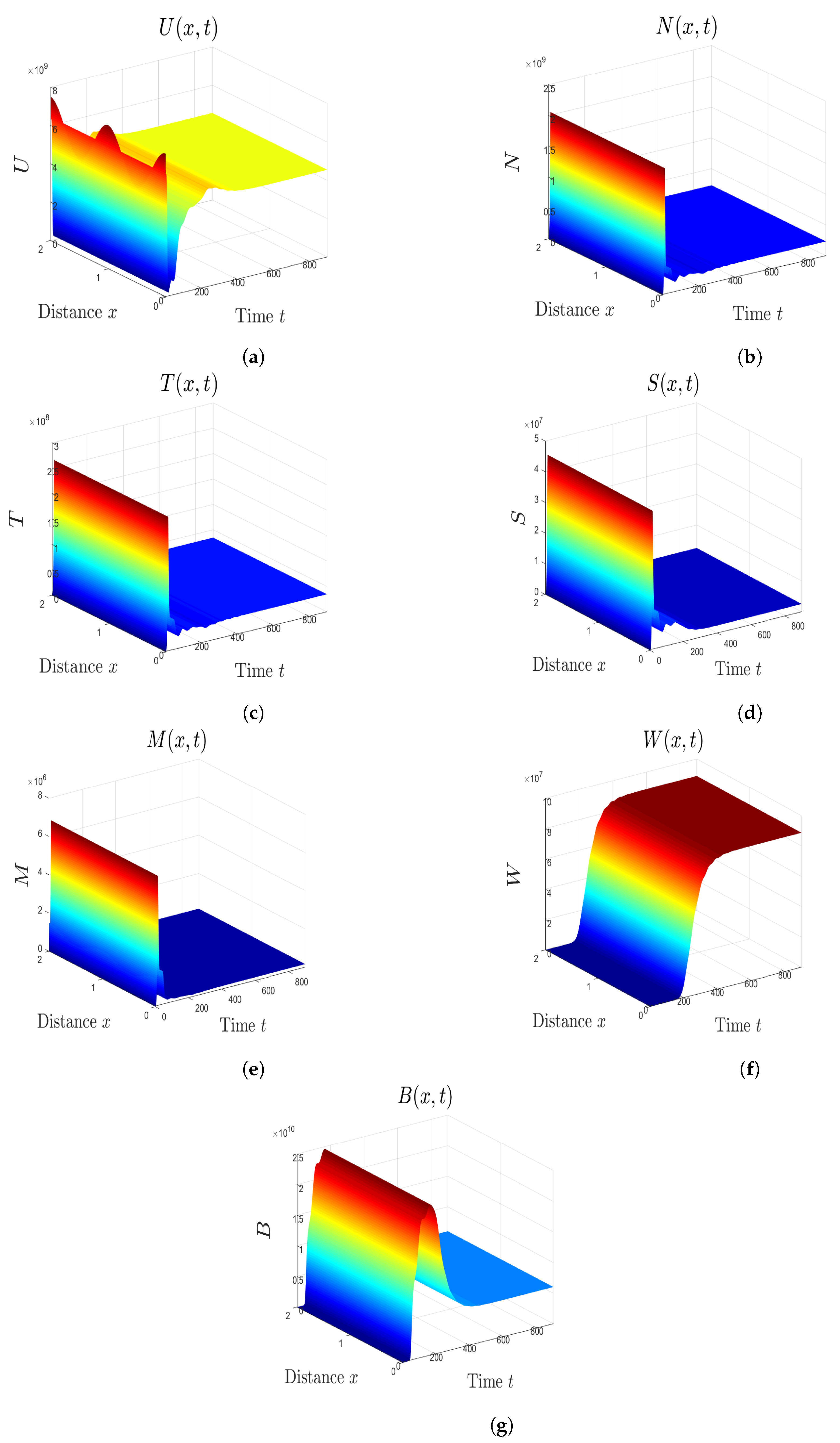
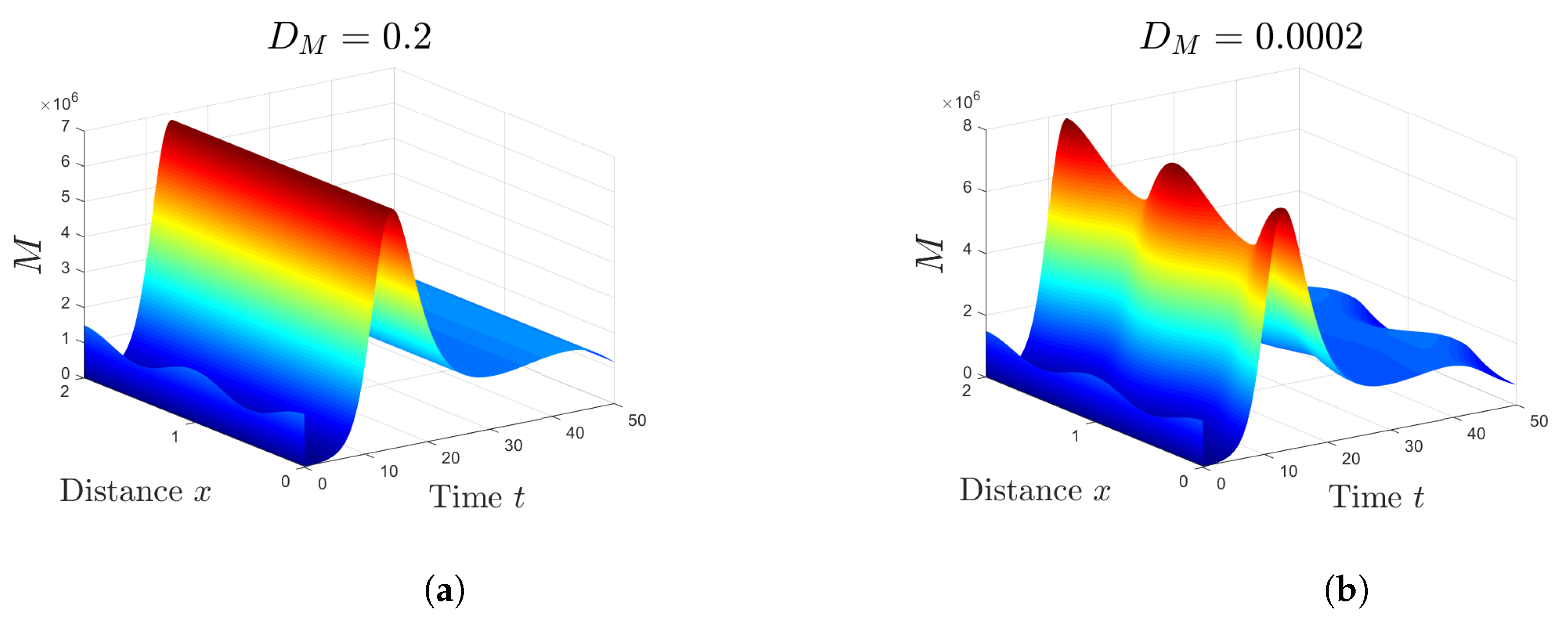
5. Numerical Simulations

In this section, we conduct some numerical simulations to illustrate the results obtained in the preceding sections. We select the spatial domain as $\Omega =[0,2]$. The space and time step sizes are selected as $\Delta x=0.02$ and $\Delta t=0.1$, respectively. The initial conditions of model (3) are considered to be the following

$$\begin{array}{cc}\hfill & U(x,0)=0.5\times {10}^{10}(1+0.5{cos}^2\left(\pi x\right))\mathrm{cells}{\mathrm{mL}}^{-1},N(x,0)=0\mathrm{cells}{\mathrm{mL}}^{-1},T(x,0)=0\mathrm{cells}{\mathrm{mL}}^{-1},\hfill \\ \hfill & S(x,0)=0\mathrm{cells}{\mathrm{mL}}^{-1},M(x,0)={10}^6(1+0.5{cos}^2\left(\pi x\right))\mathrm{cells}{\mathrm{mL}}^{-1},\hfill \\ \hfill & W(x,0)=0.0001(1+0.5{cos}^2\left(\pi x\right))\mathrm{cells}{\mathrm{mL}}^{-1},B(x,0)=0.0001(1+0.5{cos}^2\left(\pi x\right))\mathrm{cells}{\mathrm{mL}}^{-1},x\in [0,2].\hfill \end{array}$$

(35)

These values are mainly based on the values given in [26,27]. For numerical simulations, we vary the values of ${\epsilon }_1$, b, ${\epsilon }_2$, $\beta$, ${\rho }_1$, and ${\rho }_2$. The values of the rest parameters are fixed, and they are listed in Table 1. The diffusion coefficients values are taken as assumptions, while the values of the other parameters are based on values considered in the literature.

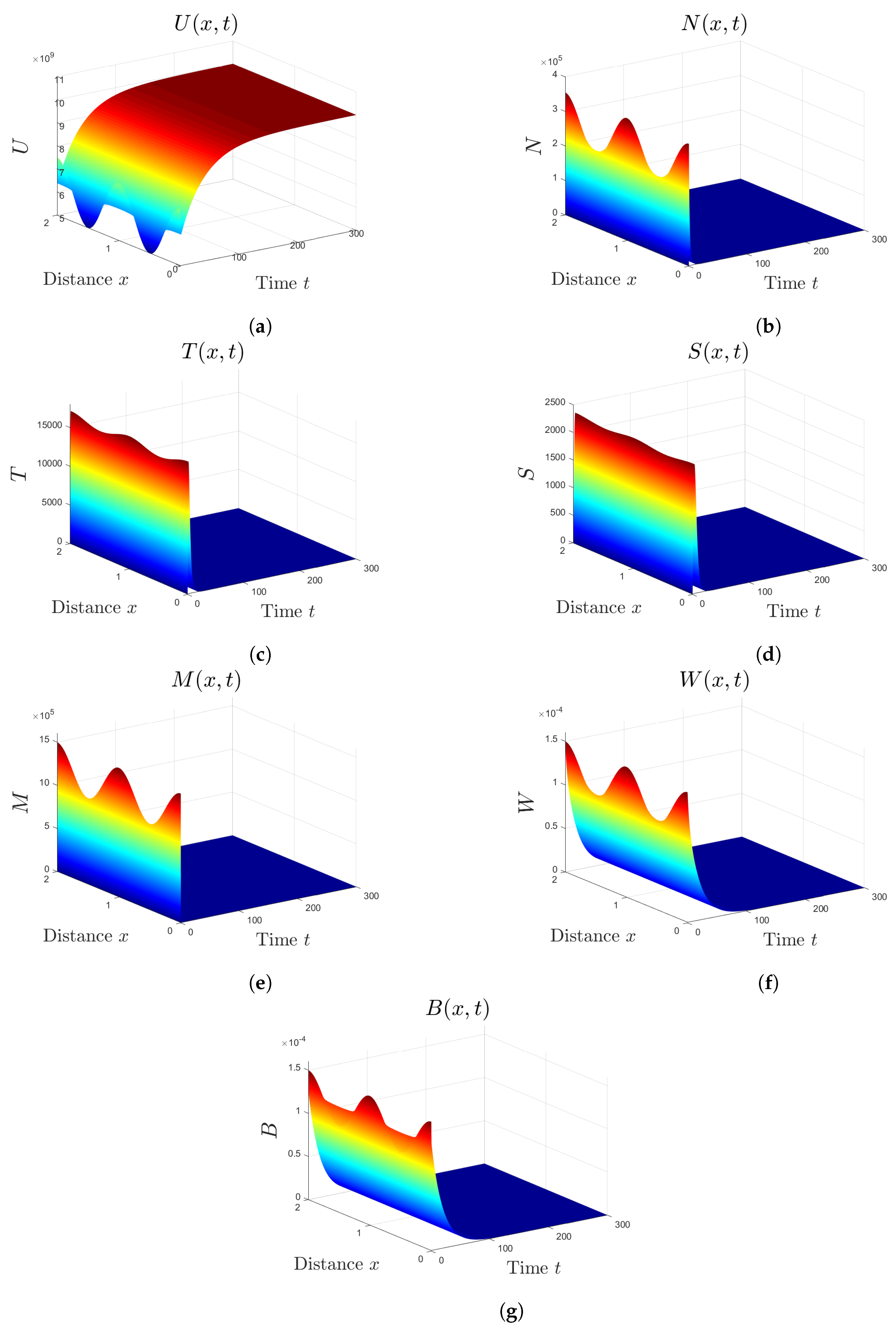
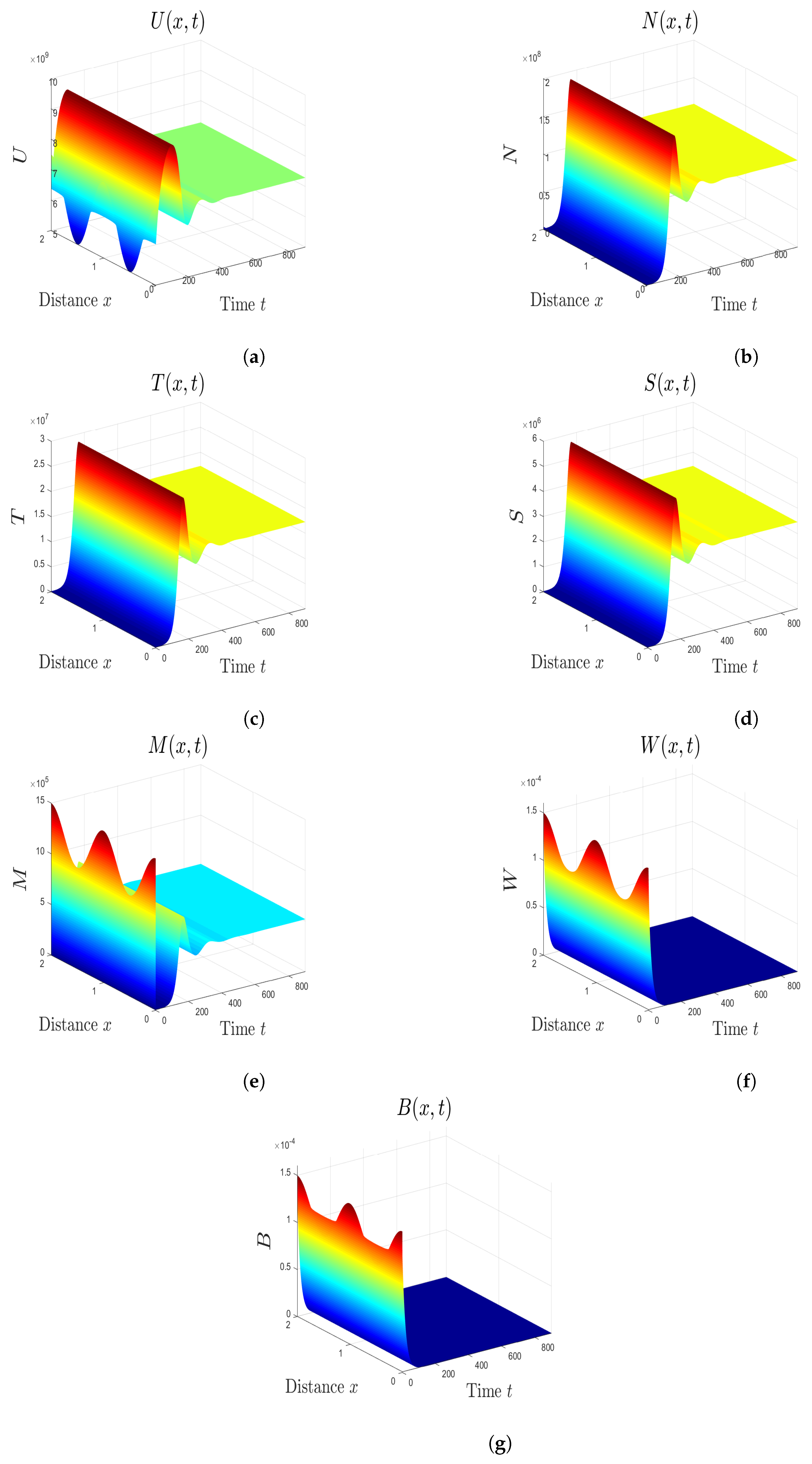
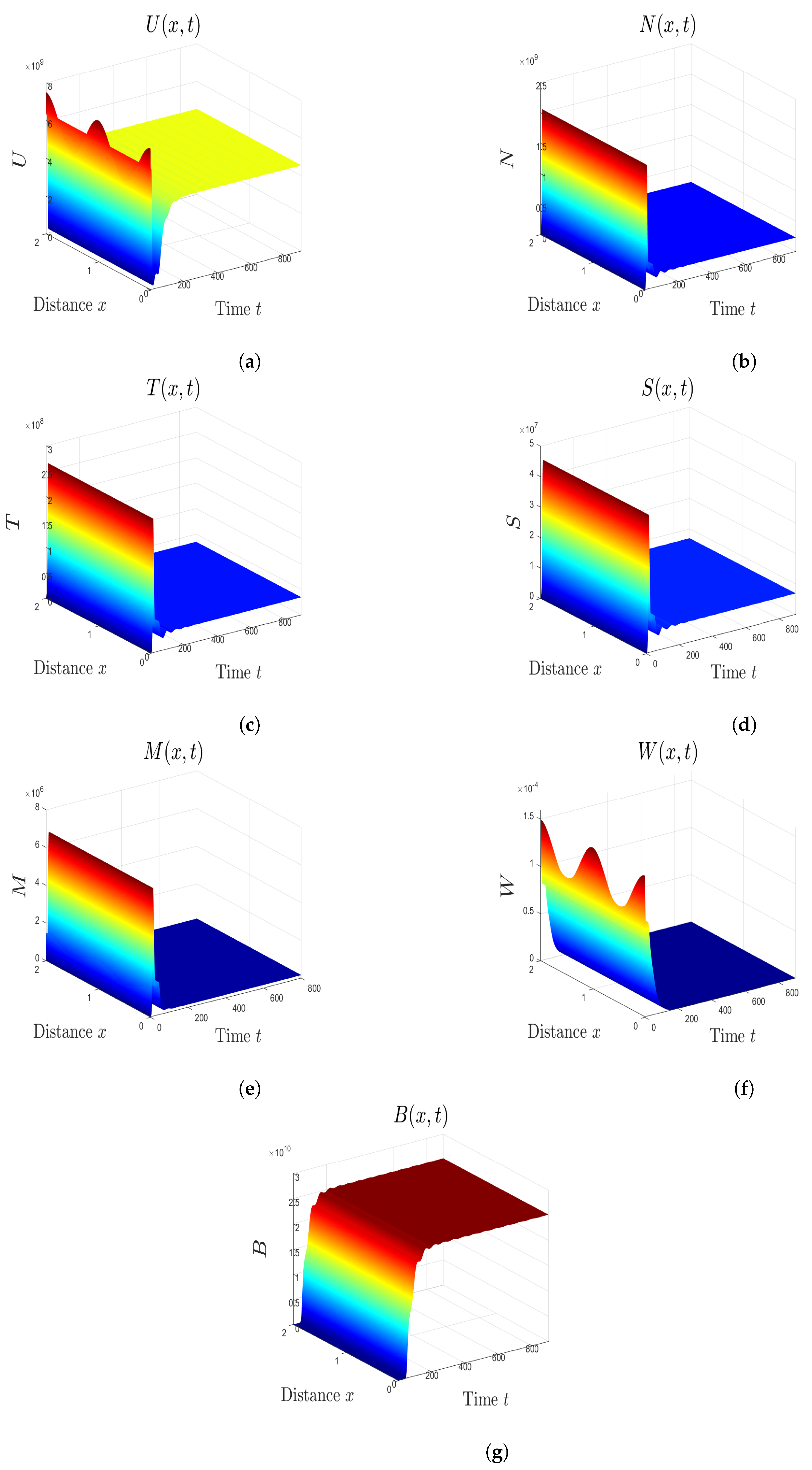
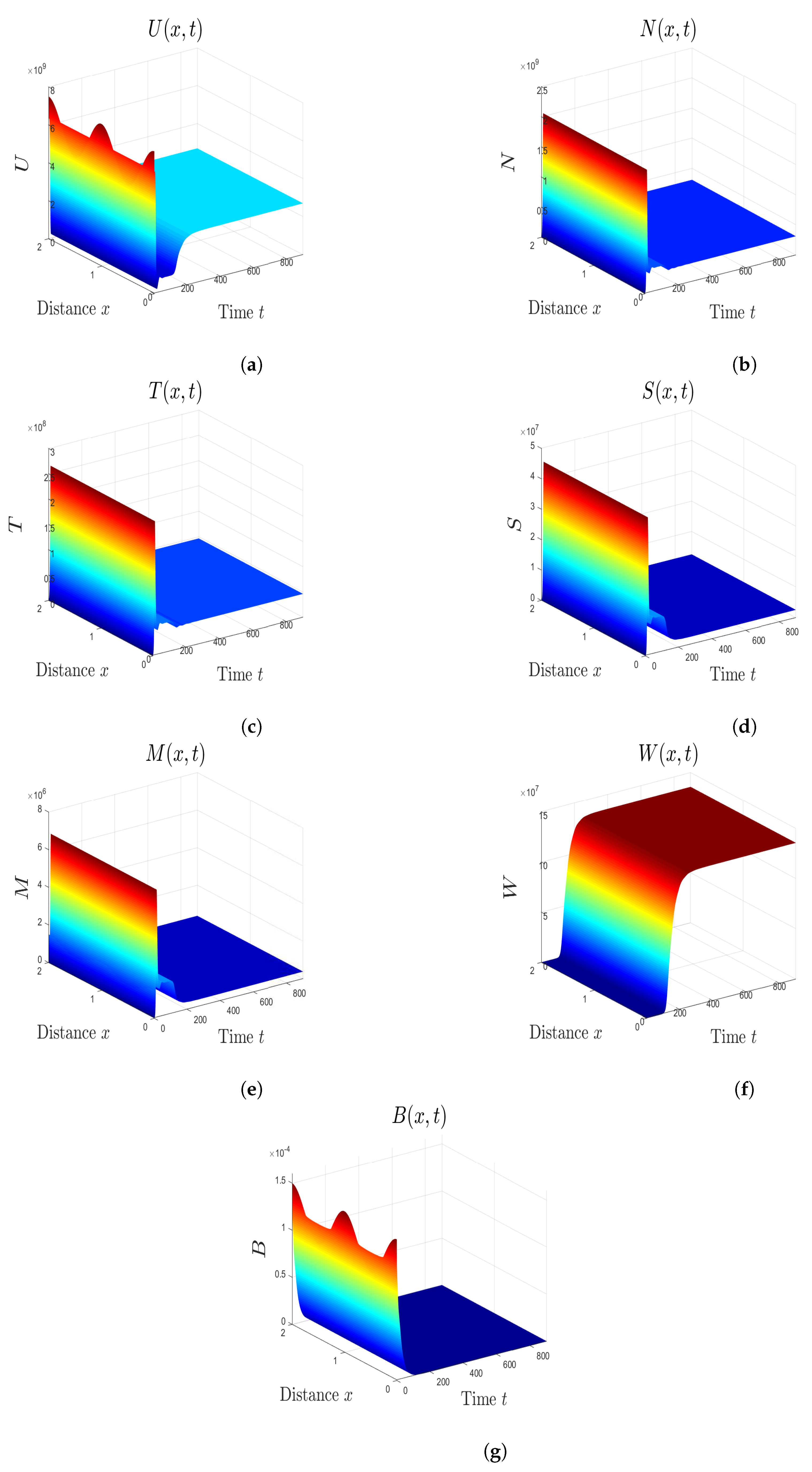
5.1. Stability of Equilibria

In this subsection, we fix the values ${\epsilon }_1=b={\epsilon }_2=0.1$. We divide the simulations into five cases corresponding to the global stability of each one of the equilibrium points as follows:

Case  1.

We consider the values $\beta =2\times {10}^{-9}$, ${\rho }_1=2\times {10}^{-8}$, and ${\rho }_2=3\times {10}^{-7}$. This gives ${\mathcal{R}}_i=0.1373<1$. The equilibrium $E_0=({10}^{10},0,0,0,0,0,0)$ is globally asymptotically stable in this situation (see Figure 1), which agrees with Theorem 3. This represents the case when the malaria infection is eliminated from the host’s body. Thus, this point is the optimal objective for antimalarial drugs.

Case  2.

We select the values $\beta =2\times {10}^{-8}$, ${\rho }_1=2\times {10}^{-9}$, and ${\rho }_2=3\times {10}^{-9}$. The threshold conditions are given by ${\mathcal{R}}_i=1.3729>1$, ${\mathcal{R}}_j=0.1056<1$, and ${\mathcal{R}}_k=0.371<1$. With these values, the equilibrium $E_1=(7.284\times {10}^9,1.151\times {10}^8,1.726\times {10}^7,3.453\times {10}^6,5.179\times {10}^5,0,0)$ is globally asymptotically stable (see Figure 2). This result coincides with the result of Theorem 4. When the CTL and antibody immune responses are not active, the malaria parasites succeed in infecting red blood cells and establishing the infection.

Case  3.

We take the values $\beta =2\times {10}^{-7}$, ${\rho }_1=2\times {10}^{-9}$, and ${\rho }_2=3\times {10}^{-7}$. The corresponding thresholds are ${\mathcal{R}}_j=6.2404>1$ and ${\mathcal{R}}_l=0.2496<1$. It follows that the equilibrium $E_2=(4.546\times {10}^9,2.308\times {10}^8,3.463\times {10}^7,6.925\times {10}^6,1.665\times {10}^5,0,2.515\times {10}^{10})$ is globally asymptotically stable (see Figure 3), which supports Theorem 5. In these circumstances, the malaria infection stimulates the production of antibodies to clear free merozoites from the blood. Nevertheless, the malaria infection persists despite the presence of both antibody immune response and blood-stage drugs.

Case  4.

We select the values $\beta =2\times {10}^{-7}$, ${\rho }_1=2\times {10}^{-8}$, and ${\rho }_2=3\times {10}^{-9}$. This gives ${\mathcal{R}}_k=3.7107>1$ and ${\displaystyle \frac{{\mathcal{R}}_j}{{\mathcal{R}}_l}}=0.0225<1$. In agreement with Theorem 6, the equilibrium $E_3=(2.703\times {10}^9,3.092\times {10}^8,4.638\times {10}^7,2.5\times {10}^6,3.75\times {10}^5,1.355\times {10}^8,0)$ is globally asymptotically stable (see Figure 4). Here, the malaria infection activates the CTL immune response to kill the schizont infected red blood cells, which decreases the count of free merozoites in the blood.

Case  5.

We take $\beta =2\times {10}^{-7}$, ${\rho }_1=2\times {10}^{-8}$, and ${\rho }_2=3\times {10}^{-7}$. This gives ${\mathcal{R}}_l=2.4961>1$ and ${\displaystyle \frac{{\mathcal{R}}_j}{{\mathcal{R}}_l}}=2.25>1$. Thus, the equilibrium $E_4=(4.545\times {10}^9,2.311\times {10}^8,3.467\times {10}^7,2.5\times {10}^6,1.667\times {10}^5,8.867\times {10}^7,6\times {10}^9)$ is globally asymptotically stable (see Figure 5), which agrees with Theorem 7. At this point, the malaria infection stimulates both the antibody immune response and CTL immune response. These responses work together to increase the concentration of uninfected cells and reduce the concentration of free merozoites and infected cells at all stages. With low treatment efficacy, the immune responses are not able to eliminate the infection.

It is worth mentioning that the global stability of the equilibrium points assures that the long time behavior of solutions is not affected by initial condition [43], i.e., for any initial conditions satisfying (4), the long time behavior of solutions will be similar to the long time behavior of solutions obtained with the initial conditions (35) and shown in Figure 1, Figure 2, Figure 3, Figure 4 and Figure 5.

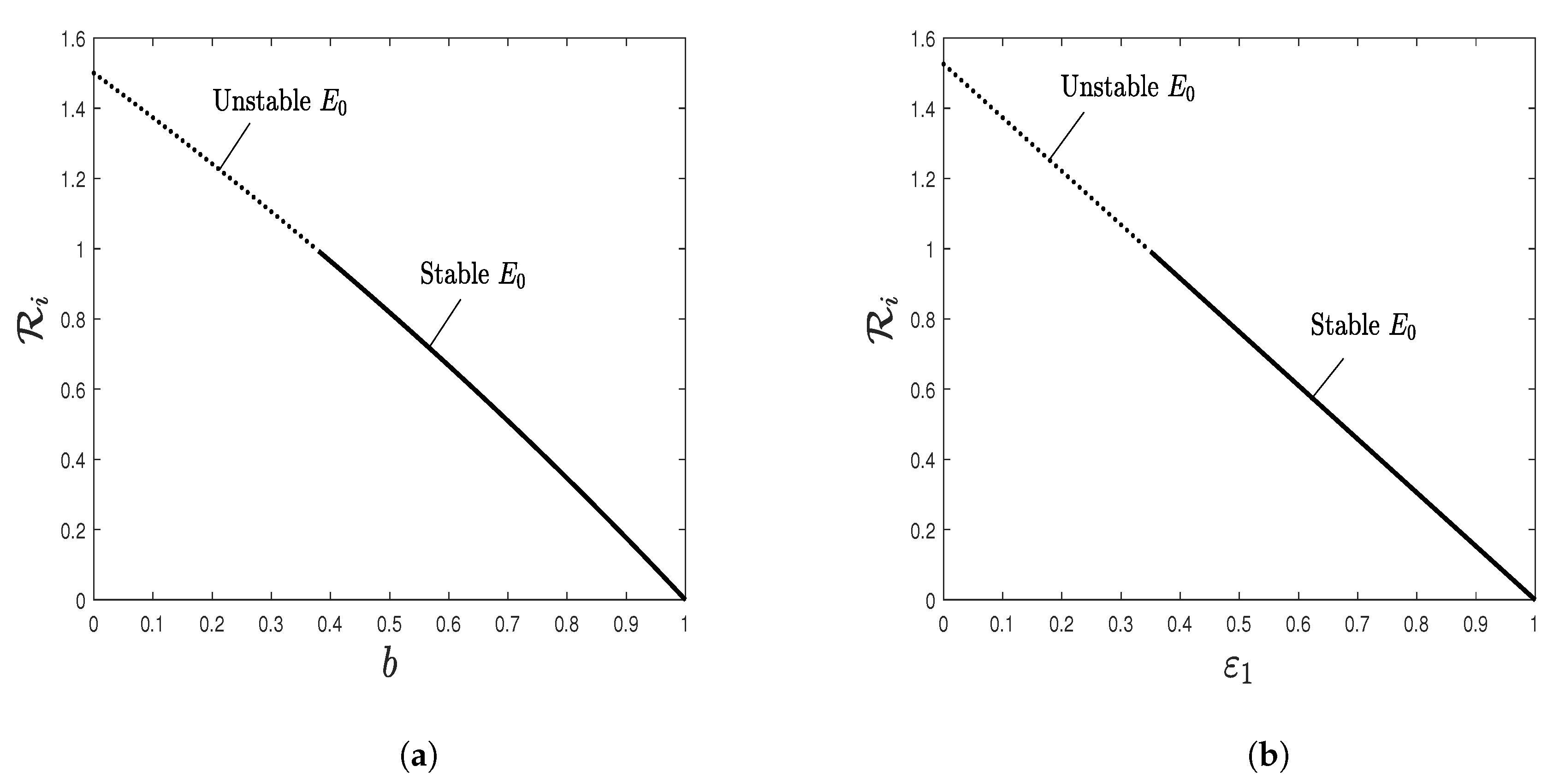
5.2. Effect of Isoleucine Starvation and Drugs on the Malaria Dynamics

To see the effect of isoleucine starvation on the stability of equilibrium points, we consider the values of the parameters $\beta =2\times {10}^{-8}$, ${\rho }_1=2\times {10}^{-9}$, ${\rho }_2=3\times {10}^{-9}$, ${\epsilon }_1=0.1$, $b=0.8$, and ${\epsilon }_2=0.1$. In this situation, we get ${\mathcal{R}}_i=0.3462<1$ which implies that the disease-free equilibrium $E_0$ is globally asymptotically stable. Mathematically, this means that increasing the value of b can decrease the value of ${\mathcal{R}}_i$ to less than one, which destabilizes $E_1$ and stabilizes $E_0$. The relation between b and ${\mathcal{R}}_i$ is depicted in Figure 6a, where ${\mathcal{R}}_i$ is drawn as a function of b. The dotted line denotes the values of b for which $E_0$ is unstable, while the solid line denotes the values of b for which $E_0$ is stable. Biologically, increasing isoleucine starvation efficacy forces the system to switch from the infection state to the malaria-free state. Accordingly, the impact of isoleucine starvation on system’s behavior can help design more effective treatments.

We can see the effect of antimalarial drugs against infection by considering the values $\beta =2\times {10}^{-8}$, ${\rho }_1=2\times {10}^{-9}$, ${\rho }_2=3\times {10}^{-9}$, ${\epsilon }_1=0.8$, $b=0.1$, and ${\epsilon }_2=0.1$. This gives ${\mathcal{R}}_i=0.3051<1$, where the disease-free equilibrium $E_0$ becomes globally asymptotically stable. Therefore, increasing the efficacy of treatment to large values decreases the infection rate and, as a result, clears the disease (see Figure 6b). A similar result can be obtained by increasing the value of ${\epsilon }_2$. Therefore, the infection can be cleared with highly effective treatments.

6. Discussion

In this paper, we investigated a reaction-diffusion model for the blood-stage dynamics of malaria infection with CTL and antibody immune responses. The model studies the interactions between uninfected erythrocytes, three types of infected red blood cells, free merozoites, CTL immune response and antibody immune response. The model contains parameters to measure the efficacy of antimalarial treatments and amino acid starvation. It has five equilibrium points:

(a)

The disease-free equilibrium $E_0$ is usually defined and globally asymptotically stable if ${\mathcal{R}}_i\le 1$. This point corresponds to the elimination of malaria infection.

(b)

The immune-free equilibrium $E_1$ is defined if ${\mathcal{R}}_i>1$, and it is globally asymptotically stable if ${\mathcal{R}}_j\le 1$ and ${\mathcal{R}}_k\le 1$. At this point, the malaria parasite P. falciparum succeeds in establishing the infection when the immune responses are not active.

(c)

The antibody-activated equilibrium $E_2$ is defined if ${\mathcal{R}}_j>1$, and it is globally asymptotically stable if ${\mathcal{R}}_l\le 1$. At this point, the antibody immune response is activated to attack the free blood merozoites.

(d)

The CTL-activated equilibrium $E_3$ is defined if ${\mathcal{R}}_k>1$, and it is globally asymptotically stable if ${\displaystyle \frac{{\mathcal{R}}_j}{{\mathcal{R}}_l}}\le 1$. At this point, the CTL immune response is activated to kill the schizont infected red blood cells.

(e)

The CTL/antibody coexistence equilibrium $E_4$ is defined and globally asymptotically stable if ${\mathcal{R}}_l>1$ and ${\displaystyle \frac{{\mathcal{R}}_j}{{\mathcal{R}}_l}}>1$. Here, the malaria infection stimulates the CTL and antibody immune responses to fight the infection.

We found that increasing isoleucine starvation efficacy b in model (3) drives the system towards the malaria-free equilibrium and, in general, affects the stability of equilibria. Thus, the perturbation in the asexual malaria life-cycle duo to isoleucine starvation can be an important target for antimalarial drugs [34]. The effectiveness of these drugs depends on the value the isoleucine starvation efficacy b could reach when these drugs are used. Isoleucine starvation was produced in vitro by exposing the parasites to isoleucine-free medium [34]. Also, protein malnutrition was produced in animal studies by feeding protein-restricted diets to malaria-infected rats [44,45]. However, the induction of isoleucine starvation in humans and its complete effect on malaria patients is still under investigation. In addition to isoleucine starvation, we found that blood-stage treatments with high efficacy (${\epsilon }_1$ and ${\epsilon }_2$) are needed to clear the infection. Hence, the values of these parameters can have a crucial impact on the disease dynamics. Furthermore, the immune responses at the CTL/antibody coexistence equilibrium $E_4$ do not clear the infection, but they reduce the concentrations of free merozoites and infected cells at the three developmental stages (rings, trophozoites, and schizonts). The presence of diffusion in model (3) does not affect the global stability of equilibria. However, it affects the behavior of solutions at the beginning of infection before reaching the equilibrium points (see Figure 7). This may have a substantial impact on the estimates of parameters describing the early infection [32]. Thus, considering spatial effects is important to get a good approximation for infection dynamics. The spatial distribution of solutions at different progressive time points can be seen more clearly by considering two-dimensional square domain [46]. Compared to the existing models of blood-stage malaria infection, our model is the first model that addresses with a detailed mathematical analysis the development of the infected red blood cells through the three main sequential stages using a reaction-diffusion model with adaptive immune response. Our model also includes the effects of antimalarial drugs and isoleucine starvation on malaria dynamics. Previous models have ignored some of these factors. The results can help design more effective treatments to fight malaria infection by taking into account some important factors that can affect the disease progression. Model (3) uses bilinear rates and ignores the effects of delays or immune responses against the ring and schizont stages. Thus, model (3) can be improved in many ways: (i) by considering more general infection and stimulation rates (see, e.g., [47,48]); (ii) by assuming CTL immune response against the three types of infected cells; (iii) by taking into account the delays that may occur in some processes during malaria infection (see, e.g., [49]); (iv) by performing a bifurcation analysis of the model (see, e.g., [50]). We leave these improvements as possible future works.

References

1. WHO. World Malaria Report 2019; License: CC BY-NC-SA 3.0 IGO; World Health Organization: Geneva, Switzerland, 2019. [Google Scholar]
2. Chen, H.; Wang, W.; Fu, R.; Luo, J. Global analysis of a mathematical model on malaria with competitive strains and immune responses. Appl. Math. Comput. 2015, 259, 132–152. [Google Scholar] [CrossRef]
3. Khoury, D.; Aogo, R.; Randriafanomezantsoa-Radohery, G.; McCaw, J.; Simpson, J.; McCarthy, J.; Haque, A.; Cromer, D.; Davenport, M. Within-host modeling of blood-stage malaria. Immun. Rev. 2018, 285, 168–193. [Google Scholar] [CrossRef]
4. Niger, A.; Gumel, A. Immune response and imperfect vaccine in malaria dynamics. Math. Popul. Stud. 2011, 18, 55–86. [Google Scholar] [CrossRef]
5. Agusto, F.; Leite, M.; Orive, M. The transmission dynamics of a within-and between-hosts malaria model. Ecol. Complex. 2019, 38, 31–55. [Google Scholar] [CrossRef]
6. Song, T.; Wang, C.; Tian, B. Mathematical models for within-host competition of malaria parasites. Math. Biosci. Eng. 2019, 16, 6623–6653. [Google Scholar] [CrossRef] [PubMed]
7. Zaloumis, S.; Humberstone, A.; Charman, S.; Price, R.; Moehrle, J.; Gamo-Benito, J.; McCaw, J.; Jamsen, K.; Smith, K.; Simpson, J. Assessing the utility of an anti-malarial pharmacokinetic-pharmacodynamic model for aiding drug clinical development. Malaria J. 2012, 11, 303. [Google Scholar] [CrossRef] [PubMed] [Green Version]
8. Nowak, M.A.; May, R.M. Virus Dynamics: Mathematical Principles of Immunology and Virology; Oxford University: Oxford, UK, 2000. [Google Scholar]
9. Ren, X.; Tian, Y.; Liu, L.; Liu, X. A reaction-diffusion within-host HIV model with cell-to-cell transmission. J. Math. Biol. 2018, 76, 1831–1872. [Google Scholar] [CrossRef] [PubMed]
10. Elaiw, A.M.; Hobiny, A.D.; Al Agha, A.D. Global dynamics of reaction-diffusion oncolytic M1 virotherapy with immune response. Appl. Math. Comput. 2020, 367, 1–21. [Google Scholar] [CrossRef]
11. Elaiw, A.M.; AlShamrani, N.H. Stability of an adaptive immunity pathogen dynamics model with latency and multiple delays. Math. Meth. Appl. Sci. 2018, 41, 6645–6672. [Google Scholar] [CrossRef]
12. Miao, H.; Teng, Z.; Abdurahman, X.; Li, Z. Global stability of a diffusive and delayed virus infection model with general incidence function and adaptive immune response. Comput. Appl. Math. 2017, 37, 3780–3805. [Google Scholar] [CrossRef]
13. Elaiw, A.M.; Elnahary, E.K. Analysis of general humoral immunity HIV dynamics model with HAART and distributed delays. Mathematics 2019, 7, 157. [Google Scholar] [CrossRef] [Green Version]
14. Elaiw, A.M.; Alshehaiween, S.F.; Hobiny, A.D. Global properties of delay-distributed HIV dynamics model including impairment of B-cell functions. Mathematics 2019, 7, 837. [Google Scholar] [CrossRef] [Green Version]
15. Elaiw, A.M.; Alshehaiween, S.F. Global stability of delay-distributed viral infection model with two modes of viral transmission and B-cell impairment. Math. Methods Appl. Sci. 2020. [Google Scholar] [CrossRef]
16. Elaiw, A.M.; AlShamrani, N.H. Stability of a general adaptive immunity virus dynamics model with multi-stages of infected cells and two routes of infection. Math. Methods Appl. Sci. 2020, 43, 1145–1175. [Google Scholar] [CrossRef]
17. Anderson, R.; May, R.; Gupta, S. Non-linear phenomena in host-parasite interactions. Parasitology 1989, 99, S59–S79. [Google Scholar] [CrossRef]
18. Anderson, R. Complex dynamic behaviours in the interaction between parasite populations and the host’s immune system. Int. J. Parasitol. 1998, 28, 551–566. [Google Scholar] [CrossRef]
19. Saul, A. Models for the in-host dynamics of malaria revisited: Errors in some basic models lead to large over-estimates of growth rates. Parasitology 1998, 117, 405–407. [Google Scholar] [CrossRef]
20. Gravenor, M.; Lloyd, A. Reply to: Models for the in-host dynamics of malaria revisited: Errors in some basic models lead to large over-estimates of growth rates. Parasitology 1998, 171, 409–410. [Google Scholar] [CrossRef] [Green Version]
21. Hoshen, M.; Heinrich, R.; Stein, W.; Ginsburg, H. Mathematical modelling of the within-host dynamics of Plasmodium falciparum. Parasitology 2000, 121, 227–235. [Google Scholar] [CrossRef]
22. Iggidr, A.; Kamgang, J.; Sallet, G.; Tewa, J. Global analysis of new malaria intrahost models with a competitive exclusion principle. SIAM J. Appl. Math. 2006, 67, 260–278. [Google Scholar] [CrossRef] [Green Version]
23. Saralamba, S.; Pan-Ngum, W.; Maude, R.; Lee, S.J.; Tarning, J.; Lindegårdh, N.; Chotivanich, K.; Nosten, F.; Day, N.; Socheat, D.; et al. Intrahost modeling of artemisinin resistance in Plasmodium falciparum. Proc. Natl. Acad. Sci. USA 2011, 108, 397–402. [Google Scholar] [CrossRef] [PubMed] [Green Version]
24. Demasse, R.; Ducrot, A. An age-structured within-host model for multistrain malaria infections. SIAM J. Appl. Math. 2013, 73, 572–593. [Google Scholar] [CrossRef] [Green Version]
25. Li, Y.; Ruan, S.; Xiao, D. The within-host dynamics of malaria infection with immune response. Math. Biosci. Eng. 2011, 8, 999–1018. [Google Scholar] [PubMed]
26. Tumwiine, J.; Mugisha, J.; Luboobi, L. On global stability of the intra-host dynamics of malaria and the immune system. J. Math. Anal. Appl. 2008, 341, 855–869. [Google Scholar] [CrossRef] [Green Version]
27. Hetzel, C.; Anderson, R. The within-host cellular dynamics of bloodstage malaria: Theoretical and experimental studies. Parasitology 1996, 113, 25–38. [Google Scholar] [CrossRef]
28. Tewa, J.; Fokouop, R.; Mewoli, B.; Bowong, S. Mathematical analysis of a general class of ordinary differential equations coming from within-hosts models of malaria with immune effectors. App. Math. Comput. 2012, 2018, 7347–7361. [Google Scholar] [CrossRef]
29. Tchinda, P.; Tewa, J.; Mewoli, B.; Bowong, S. Mathematical analysis of a general class of intra-host model of malaria with “allee effect“. J. Nonl. Syst. Appl. 2013, 36, 52. [Google Scholar]
30. Cai, L.; Tuncer, N.; Martcheva, M. How does within-host dynamics affect population-level dynamics? Insights from an immuno-epidemiological model of malaria. Math. Methods Appl. Sci. 2017, 40, 6424–6450. [Google Scholar] [CrossRef]
31. Orwa, T.; Mbogo, R.; Luboobi, L. Mathematical model for the in-host malaria dynamics subject to malaria vaccines. Lett. Biomath. 2018, 5, 222–251. [Google Scholar] [CrossRef] [Green Version]
32. Funk, G.; .Jansen, V.A.A.; Bonhoeffer, S.; Killingback, T. Spatial models of virus-immune dynamics. J. Theor. Biol. 2005, 233, 221–236. [Google Scholar] [CrossRef]
33. Takoutsing, E.; Temgoua, A.; Yemele, D.; Bowong, S. Dynamics of an intra-host model of malaria with periodic antimalarial treatment. Int. J. Nonl. Sci. 2019, 27, 148–164. [Google Scholar]
34. Babbitt, S.; Altenhofen, L.; Cobbold, S.; Istvan, E.; Fennell, C.; Doerig, C.; Llinas, M.; Goldberg, D. Plasmodium falciparum responds to amino acid starvation by entering into a hibernatory state. Proc. Natl. Acad. Sci. USA 2012, 109, E3278–E3287. [Google Scholar] [CrossRef] [PubMed] [Green Version]
35. Zhang, Y.; Xu, Z. Dynamics of a diffusive HBV model with delayed Beddington-DeAngelis response. Nonl. Anal. Real World Appl. 2014, 15, 118–139. [Google Scholar] [CrossRef]
36. Xu, Z.; Xu, Y. Stability of a CD4+ T cell viral infection model with diffusion. Int. J. Biomath. 2018, 11, 1–16. [Google Scholar] [CrossRef]
37. Smith, H.L. Monotone Dynamical Systems: An Introduction to the Theory of Competitive and Cooperative Systems; American Mathematical Society: Providence, RI, USA, 1995. [Google Scholar]
38. Protter, M.H.; Weinberger, H.F. Maximum Principles in Differential Equations; Prentic Hall: Englewood Cliffs, NJ, USA, 1967. [Google Scholar]
39. Henry, D. Geometric Theory of Semilinear Parabolic Equations; Springer: New York, NY, USA, 1993. [Google Scholar]
40. Hattaf, K.; Yousfi, N. Global stability for reaction-diffusion equations in biology. Comput. Math. Appl. 2013, 66, 1488–1497. [Google Scholar] [CrossRef]
41. Hsu, S. A survey of constructing lyapunov functions for mathematical models in population biology. Taiwan. J. Math. 2005, 9, 151–173. [Google Scholar] [CrossRef]
42. Hale, J.K.; Verduyn Lunel, S.M. Introduction to Functional Differential Equations; Springer: New York, NY, USA, 1993. [Google Scholar]
43. Khalil, H.K. Nonlinear Systems; Prentice-Hall: New Jersey, NJ, USA, 1996. [Google Scholar]
44. Bakker, N.; Eling, W.; De Groot, A.; Sinkeldam, E.; Luyken, R. Attenuation of malaria infection, paralysis and lesions in the central nervous system by low protein diets in rats. Acta Trop. 1992, 50, 285–293. [Google Scholar] [CrossRef]
45. Edirisinghe, J.; Fern, E.; Targett, G. Resistance to superinfection with Plasmodium berghei in rats fed a protein-free diet. Trans. R Soc. Trop. Med. Hyg. 1982, 76, 382–386. [Google Scholar] [CrossRef]
46. Sun, H.; Wang, J. Dynamics of a diffusive virus model with general incidence function, cell-to-cell transmission and time delay. Comput. Math. Appl. 2019, 77, 284–301. [Google Scholar] [CrossRef]
47. Elaiw, A.M.; Raezah, A.A. Stability of general virus dynamics models with both cellular and viral infections and delays. Math. Methods Appl. Sci. 2017, 40, 5863–5880. [Google Scholar] [CrossRef]
48. Elaiw, A.M.; AlShamrani, N.H. Global stability of a delayed adaptive immunity viral infection with two routes of infection and multi-stages of infected cells. Commun. Nonl. Sci. Num. Simul. 2020, 86, 1–27. [Google Scholar] [CrossRef]
49. Elaiw, A.M.; AlAgha, A.D. Analysis of a Delayed and Diffusive Oncolytic M1 Virotherapy Model with Immune Response; Nonlinear Analysis: Real World Applications; Article 103116; Elsevier: Amsterdam, The Netherlands, 2020. [Google Scholar] [CrossRef]
50. Luo, J.; Wang, W.; Chen, H.; Fu, R. Bifurcations of a mathematical model for HIV dynamics. J. Math. Anal. Appl. 2016, 434, 837–857. [Google Scholar] [CrossRef]
Figure 1. The numerical simulations of model (3) when R i 1 . The disease-free equilibrium E 0 is globally asymptotically stable. The subfigures show the spatiotemporal behaviors of (a) uninfected red blood cells U, (b) ring infected red blood cells N, (c) trophozoite infected red blood cells T, (d) schizont infected red blood cells S, (e) free merozoites M, (f) CTLs W, and (g) antibodies B.
Mathematics 08 00563 g001
Figure 2. The numerical simulations of model (3) when R i > 1 , R j 1 , and R k 1 . The immune-free equilibrium E 1 is globally asymptotically stable. The subfigures show the spatiotemporal behaviors of (a) uninfected red blood cells U, (b) ring infected red blood cells N, (c) trophozoite infected red blood cells T, (d) schizont infected red blood cells S, (e) free merozoites M, (f) CTLs W, and (g) antibodies B.
Mathematics 08 00563 g002
Figure 3. The numerical simulations of model (3) when R j > 1 and R l 1 The antibody-activated equilibrium E 2 is globally asymptotically stable. The subfigures show the spatiotemporal behaviors of (a) uninfected red blood cells U, (b) ring infected red blood cells N, (c) trophozoite infected red blood cells T, (d) schizont infected red blood cells S, (e) free merozoites M, (f) CTLs W, and (g) antibodies B.
Mathematics 08 00563 g003
Figure 4. The numerical simulations of model (3) when R k > 1 and R j R l 1 The CTL-activated equilibrium E 3 is globally asymptotically stable. The subfigures show the spatiotemporal behaviors of (a) uninfected red blood cells U, (b) ring infected red blood cells N, (c) trophozoite infected red blood cells T, (d) schizont infected red blood cells S, (e) free merozoites M, (f) CTLs W, and (g) antibodies B.
Mathematics 08 00563 g004
Figure 5. The numerical simulations of model (3) when R l > 1 and R j R l > 1 The coexistence equilibrium E 4 is globally asymptotically stable. The subfigures show the spatiotemporal behaviors of (a) uninfected red blood cells U, (b) ring infected red blood cells N, (c) trophozoite infected red blood cells T, (d) schizont infected red blood cells S, (e) free merozoites M, (f) CTLs W, and (g) antibodies B.
Mathematics 08 00563 g005
Figure 6. The effect of varying the efficacy of blood-stage treatment ε 1 and the efficacy of isoleucine starvation b on the within-host basic reproductive number R i The dotted line denotes the values of b for which E 0 is unstable, while the solid line denotes the values of b for which E 0 is stable. (a) R i is a nonlinear function of b, where increasing the value of b causes the disease-free equilibrium E 0 to become stable at approximately b = 0.375 . (b) R i is a linear function of ε 1 where increasing the value of ε 1 causes the disease-free equilibrium E 0 to become stable at approximately ε 1 = 0.344 .
Mathematics 08 00563 g006
Figure 7. The effect of changing the diffusion coefficient on the concentration of free merozoites M at the beginning of infection. All parameters are identical to those used in Figure 5, while the diffusion coefficient D M is changed from (a) D M = 0.2 to (b) D M = 0.0002 .
Mathematics 08 00563 g007