Sensitivity Analysis of Mathematical Model to Study the Effect of T Cells Infusion in Treatment of CLL

Abstract

In this paper, we considered a mathematical model concerned with the treatment of Chronic Lymphocytic Leukemia (CLL) taking into account the effect of superficially infused T cells in this particular type of tumor. The model is described thoroughly by the system of non-linear differential equations explaining the interaction of naïve, infected, cancer and immune cell population. The detailed sensitivity analysis with the application is the major part of this paper. The basic objective is to provide insight to how parameters’ behavior varies model results by elaborating the results obtained from the application of sensitivity analysis. The sensitivity of the model was evaluated not only theoretically, but also with the help of a numerical approach, producing graphs providing better imminent of results. We argue that the application of the sensitivity analysis method endows an insight into how and which parameters are of primary significance in controlling the spread of leukemia.

1. Introduction

The inherited concept of irrelevance of mathematics and biology has been changed to a great extent, somewhat because of the realization of the scientific world [1] of the undeniable services of mathematics in helping to gain a better understanding of various biological phenomena occurring in nature on daily basis. Mathematicians feel pleased and proud of their being praised by other scientists due to the role of mathematics in biology. Mathematical modeling is a remarkable example of the healthy support provided by mathematicians for better understanding [2,3,4]. Even complex biological models can be better understood by computational and mathematical models [5,6,7].

Millions of people’s lives are in danger due to cancer throughout the world. There are many definitions of cancer available in the literature but the simplest one is the out of control development and splitting up of dungeons. There are several types of tumor, among which one is known as Leukemia, usually known as blood cancer [8]. This disease starts from blood stem cells. These cells are assumed to grow either as lymphoid or myeloid branch cells. The scheme of growth of Lymphoid Stem Cells (LSC) is as follows: these grow into lymphocytes, a type of white corpuscle acting to boost the body immune sense, which helps encounter viruses and wipe out unusual cells, whereas Myeloid Stem Cells (MSC) breed as erythrocyte and thrombocytes. Erythrocytes award oxygen to all tissues and thrombocytes form clots to avoid hemorrhage [9,10]. As the stem cells grow, these become blast cells, known to be undeveloped blood cells. In leukemia, there is an overproduction of these cells. These cells keep on multiplying without any bound and do not become mature ones in the long run. This multiplication of abnormal cells then stops not only the proper functioning of normal cells, but also the normal distribution of the remaining standard cells, which, in turn, gives rise to tumor, and such persons are diagnosed as Leukemic patients.

The explanation of the physiology of the Lymphatic System in body homeostasis is of prime importance for better understanding the causes of Chronic Lymphocytic Leukemia. The main components of the lymphatic system are immigration dendritic cells, a type of white blood cell called macrophages, lymph, lymphatic vessels, lymphoid tissues, lymphocytes, and phagocytes. Lymphatic system has two basic sections; one is known as peripheral and the second as central [11].

The basic function of this system is to transfer lymph all over the body and also provide support to throw out waste and unnecessary material. The key function of the lymphatic system is to provide enhanced immunity to fight against cancer [12,13].

A sufficiently large number of people have been diagnosed with leukemia tumors. According to very recent research, a total of 60,300 new cases were registered, including 35,030 males and 25,270 females in this total, and a number of deaths up to 24,370, including 14,270 males and 10,100 females. This research has been carried out by the United States, with results published under an article titled “Estimated new cancer cases and deaths by sex, United States 2018” [14,15].

A variety of treatment options are accessible, that generally include chemotherapy, targeted therapy, radiation therapy, and stem cell transplant [16,17]. Though all the methods mentioned above have been used to treat cancer for many years, each of these treatments have some side effects associated with them. To avoid these unwanted side effects, scientists found a new way of treating tumor, known as Adoptive Immunotherapy [18,19]. This is a category of immunotherapy in which leukocytes are united with a nature-produced augmentation aspect to enhance their cancer fighting capability [20]. The sole purpose of this practice is to boost the immune response of that individual [21].

Mathematical models are brought into service to estimate various, highly complex engineering, physical, environmental, social, economic and biological phenomena. Mathematical modeling plays a vital role as it adds to the ability to understand the true nature of the problem and also to predict system behavior that will, in turn, define the problem and its solution in a physical sense. Many syndromes have been studied in which the spread of an infection takes place from cell to cell. Many scientists and mathematicians have considered cancer treatment by immunotherapy, treating normal and cancer cells as competitors [22]. Many mathematical models have been developed and studied that show competition between tumors and immune system, considering the role of antibodies.

The model under study is a mathematical model consisting of four nonlinear differential equations that describe the change in the population of naïve, infected, cancerous and immune cells with respect to time, which studies the spread of leukemia with the consequence of outdoor engineered T cells’ permutation in cancer patients. The model also considers blood transfusion, as it is much needed in the treatment of cancer patients [23].

Sensitivity analysis is defined to be the study of how the ambiguity in the output of a model can be distributed to different sources of doubt in its input. It can alternatively be defined as the methodical exploration of model reaction to either (1) the perturbation of the model’s quantitative cause (e.g., input and/or parameters), or (2) a distinction in the model’s qualitative aspects (e.g., arrangement, connectivity). Model constraints with most influence on the model results are recognized through ‘Sensitivity Analysis’ [24,25]. In this paper, we applied sensitivity analysis in a local sense (one input is varied by a small amount at a time while keeping the others fixed) to the mathematical model of chronic lymphocytic leukemia [26], with immunotherapy technique application to predict the behavior of all the populations and, in particular cancer, and immune cell population. These are of prime importance in learning how the change in the input parameters causes a change in the output of the model, and what kind of change it is.

2. Materials and Methods

To advance healing either by indicating the spaces in the model where improvements could be made or by optimizing the offered therapies is the key objective of mathematical modeling, which, in turn, encourages mathematicians to form improve novel therapies. The model under argument assumes the spread of leukemia in a blood-circulating system. Let $x$ be the population of susceptible, $y$ be the population of dysfunctional blood cells, $c_s$ is the population of leukemic and $z$ is the population of immune cells [23]. The endemic model is proposed as follows:

$$\begin{array}{l}\frac{dx}{dt}=A-a_{0}x-\beta x{c}_s\\ \frac{dy}{dt}=\beta x{c}_s-{\beta }_{0}y\\ \frac{d{c}_s}{dt}=k-k_0{c}_s-k_1{c}_{s}z\\ \frac{dz}{dt}=B+b{c}_s-b_{0}z-b_{1}z{c}_s\end{array}$$

(1)

2.1. Nomenclature

Since we will be discussing the sensitivity of all of these parameters throughout, it is of prime importance to provide details of what a parameter means. Below is a list providing a description of the parameters.

$A:$

Employment rate of naive blood cells inflowing into circulatory blood from different sections as well as from blood transfusion;

$a_0:$

Natural death rate of susceptible blood cells;

$\beta :$

Decay rate of naive cells killed upon contact with tumor cells and becoming dysfunctional;

${\beta }_0:$

Natural death rate of infected cells;

$k:$

Recruitment rate of cancer cells into blood system;

$k_0:$

Normal death rate of malignant cells;

$k_1:$

Loss of cancer cells due to encounter with immune cells;

$B:$

Rate of external intravenous re-infusion of T cells;

$b:$

Propagation rate of resistant cells in case of cancer setback;

$b_0:$

Natural death rate of immune cells;

$b_1:$

Loss rate of immune cells due to encounter with cancer cells.

Now, we will discuss the method in the formal way. As we are going to apply a sensitivity analysis, before applying it to the mathematical model, we state some basic definition and produce the understanding of the sensitivity of a parameter in terms of mathematical equation. This method of computing sensitivity will be adopted throughout.

2.2. Sensitivity Analysis

The procedure used to find out how self-determining variable values will influence a particular dependent variable under a specified set of hypotheses is defined as sensitivity analysis. It is also known as the what-if analysis. The basic principle of this analysis is “change the model and observe the behavior”. The technique employed in this paper is local sensitivity analysis, derivative-based method. Local sensitivity is also known as one-factor-at-a-time (OFAT) technique and this involves (1) affecting one input variable, keeping others at their baseline values, (2) returning the variable to its nominal value, then repeating this for each of the other inputs in the same way. Now, we state the basic technique employed in this paper as follows.

The classical sensitivity of $y$ with respect to $p$ at $p_0$ is defined as

$${\sigma }_{y_0}=\underset{\Delta p\to 0}{\lim }\left(\frac{\frac{\Delta y}{y_0}}{\frac{\Delta p}{p_0}}\right)=\underset{\Delta p\to 0}{\lim }\left(\frac{p_0}{y_0}\frac{\Delta y}{\Delta p}\right)=\frac{p_0}{y_0}{y}^{\prime }(p_0)$$

(2)

where the sensitivity of naïve, infected, cancer and immune cells with respect to all parameters is given by $y^{\prime }\left(p_0\right)$ of eth formal definition of $\left(2\right)$.

This will give us the effect of variation in parameters on the model output, i.e., $y=y(p)$.

Without presenting the complete procedure opted, sensitivity equations of various parameters, after employing the sensitivity definition $\left(2\right)$, are listed as follows.

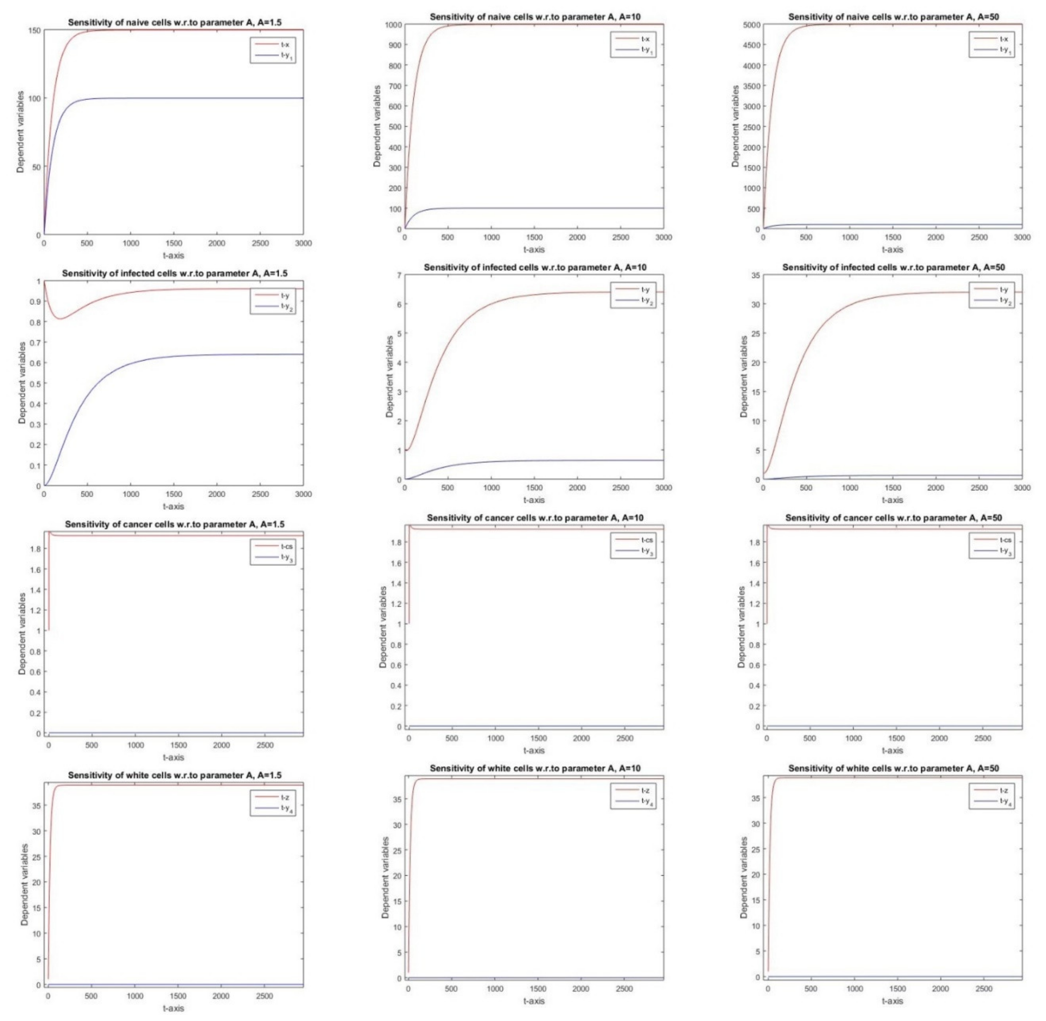
2.2.1. Sensitivity Analysis with Respect to Parameter A

This term $‘\frac{\partial y}{\partial A}’$ provides much-needed sensitivity equations.

We define

$$y_1=\frac{\partial x}{\partial A},y_2=\frac{\partial y}{\partial A},y_3=\frac{\partial c_s}{\partial A},y_4=\frac{\partial z}{\partial A}$$

$$\begin{array}{c}{\dot{y}}_1\left(t\right)=1-(a_0+\beta c_s)y_1-\beta x{y}_3\hfill \\ {\dot{y}}_2\left(t\right)=\beta x{y}_3+\beta c_s{y}_1-{\beta }_0{y}_2\hfill \\ {\dot{y}}_3\left(t\right)=-(k_0+k_{1}z)y_3-k_1{c}_s{y}_4\hfill \\ {\dot{y}}_4\left(t\right)=(b-b_{1}z)y_3-(b_0+b_1{c}_s)y_4\hfill \end{array}$$

(3)

Equation $\left(3\right)$ shows the sensitivity expression with respect to parameter $‘A’$.

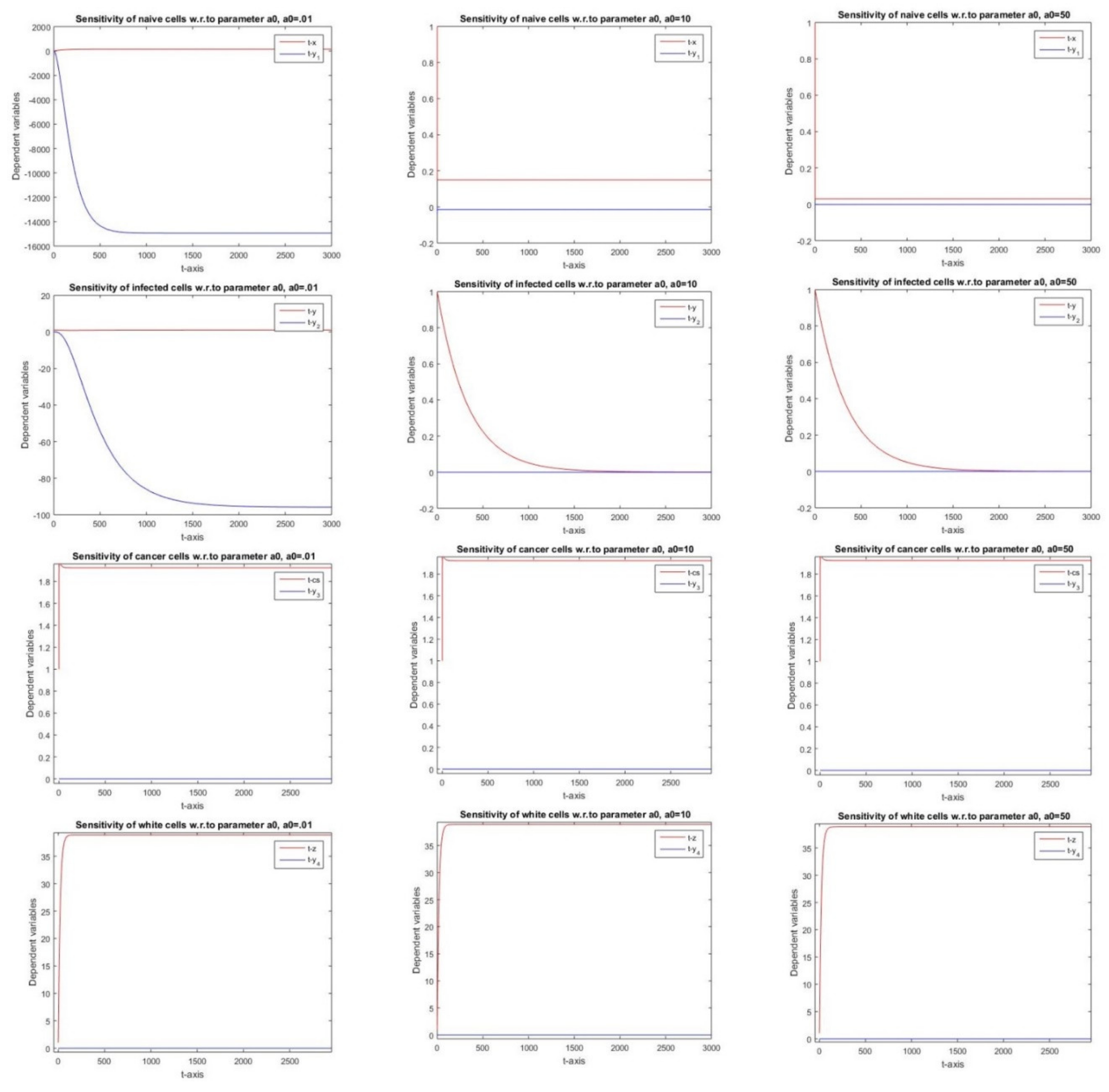
2.2.2. Sensitivity with Respect to Parameter a₀

This term $‘\frac{\partial y}{\partial a_0}’$ provides the much-needed sensitivity equations.

We define

$$y_1=\frac{\partial x}{\partial a_0},y_2=\frac{\partial y}{\partial a_0},y_3=\frac{\partial c_s}{\partial a_0},y_4=\frac{\partial z}{\partial a_0}$$

$$\begin{array}{c}{\dot{y}}_1\left(t\right)=-a_0{y}_1-x-\beta y_1{c}_s-\beta x{y}_3\hfill \\ {\dot{y}}_2\left(t\right)=\beta x{y}_3+\beta c_s{y}_1-{\beta }_0{y}_2\hfill \\ {\dot{y}}_3\left(t\right)=-k_0{y}_3-k_1{c}_s{y}_4-k_{1}z{y}_3\hfill \\ {\dot{y}}_4\left(t\right)=b{y}_3-b_0{y}_4-b_{1}z{y}_3-b_1{c}_s{y}_4\hfill \end{array}$$

(4)

Equation $\left(4\right)$ shows the sensitivity expression with respect to parameter $‘a_0’$.

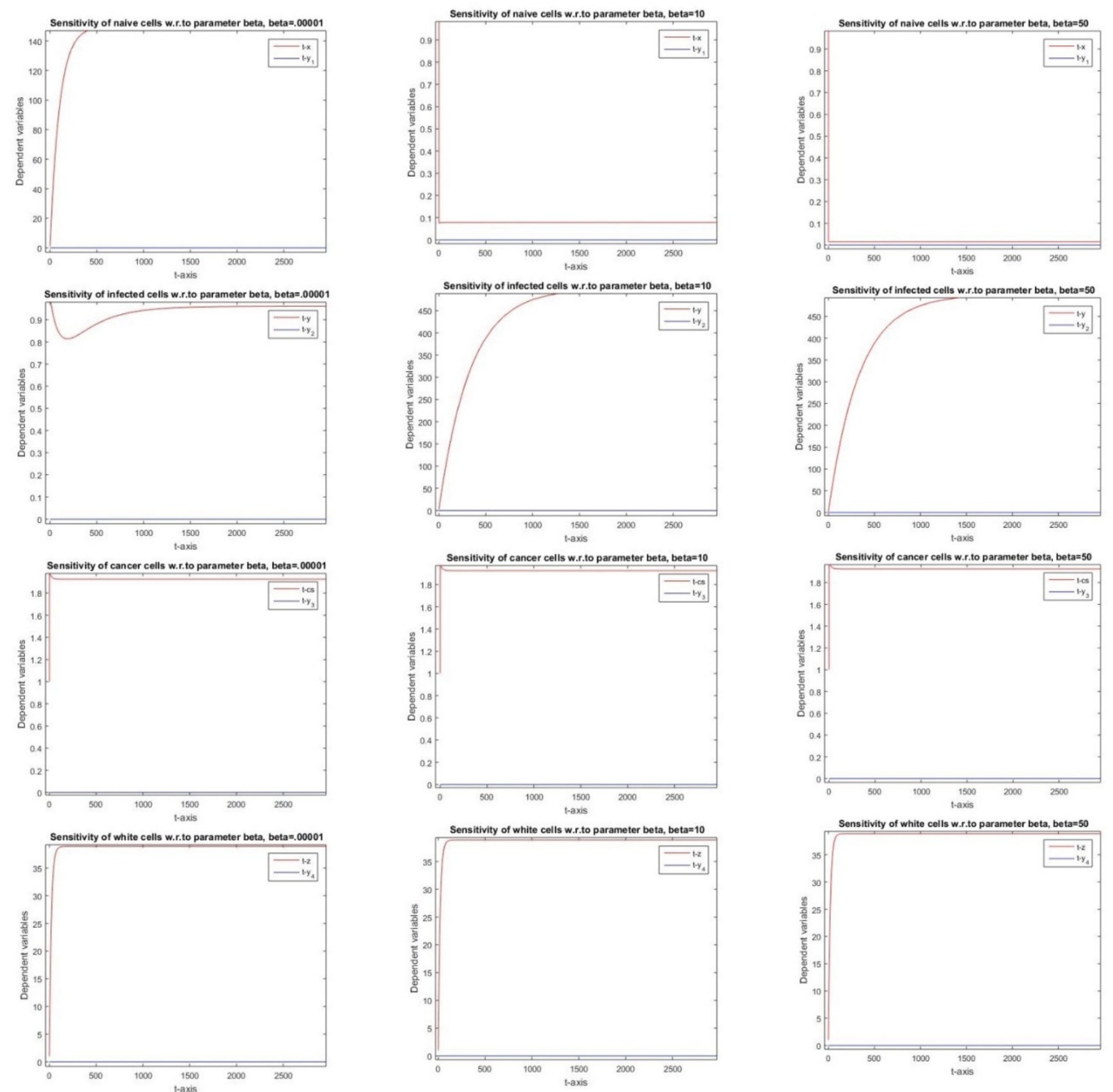
2.2.3. Sensitivity with Respect to Parameter β

This term $‘\frac{\partial y}{\partial \beta }’$ provides the much-needed sensitivity equations.

We define

$$y_1=\frac{\partial x}{\partial \beta },y_2=\frac{\partial y}{\partial \beta },y_3=\frac{\partial c_s}{\partial \beta },y_4=\frac{\partial z}{\partial \beta }$$

$$\begin{array}{c}{\dot{y}}_1\left(t\right)=-a_0{y}_1-\beta x{y}_3-\beta c_s{y}_1\hfill \\ {\dot{y}}_2\left(t\right)=\beta x{y}_3+\beta c_s{y}_1-{\beta }_0{y}_2\hfill \\ {\dot{y}}_3\left(t\right)=-k_0{y}_3-k_1{c}_s{y}_4-k_{1}z{y}_3\hfill \\ {\dot{y}}_4\left(t\right)=b{y}_3-b_0{y}_4-b_1{c}_s{y}_4-b_{1}z{y}_3\hfill \end{array}$$

(5)

Equation $\left(5\right)$ shows the sensitivity expression with respect to parameter $‘\beta ’$.

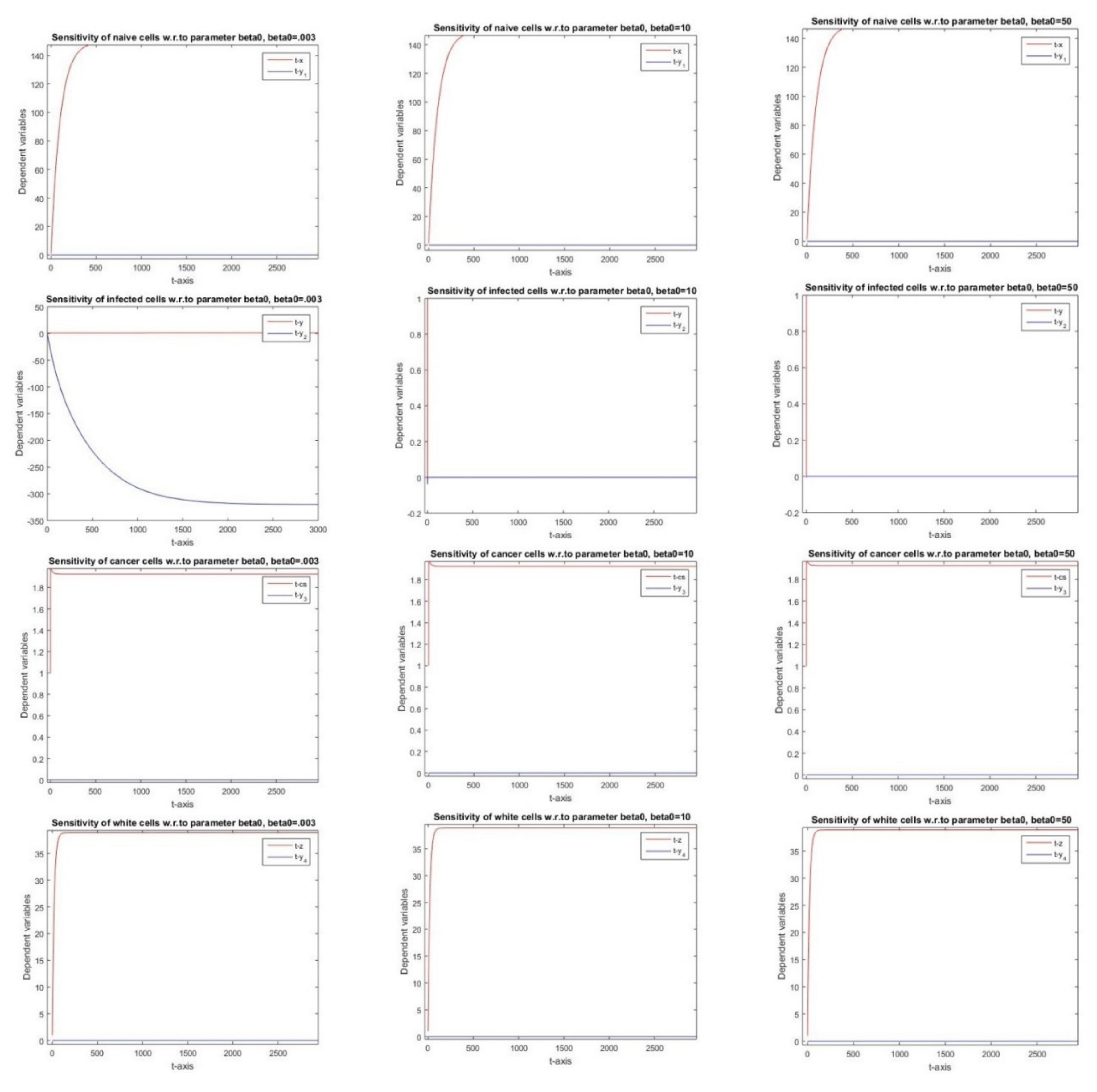
2.2.4. Sensitivity with Respect to Parameter β₀

This term $‘\frac{\partial y}{\partial {\beta }_0}’$ provides the much-needed sensitivity equations.

We define

$$y_1=\frac{\partial x}{\partial {\beta }_0},y_2=\frac{\partial y}{\partial {\beta }_0},y_3=\frac{\partial c_s}{\partial {\beta }_0},y_4=\frac{\partial z}{\partial {\beta }_0}$$

$$\begin{array}{c}{\dot{y}}_1\left(t\right)=-a_0{y}_1-\beta x{y}_3-\beta c_s{y}_1\hfill \\ {\dot{y}}_2\left(t\right)=\beta x{y}_3+\beta c_s{y}_1-{\beta }_0{y}_2-y\hfill \\ {\dot{y}}_3\left(t\right)=-k_0{y}_3-k_1{c}_s{y}_4-k_{1}z{y}_3\hfill \\ {\dot{y}}_4\left(t\right)=b{y}_3-b_0{y}_4-b_1{c}_s{y}_4-b_{1}z{y}_3\hfill \end{array}$$

(6)

Equation $\left(6\right)$ shows the sensitivity expression with respect to parameter $‘{\beta }_0’$.

2.2.5. Sensitivity with Respect to Parameter k

This term $‘\frac{\partial y}{\partial k}’$ provides the much-needed sensitivity equations.

We define

$$y_1=\frac{\partial x}{\partial k},y_2=\frac{\partial y}{\partial k},y_3=\frac{\partial c_s}{\partial k},y_4=\frac{\partial z}{\partial k}$$

$$\begin{array}{c}{\dot{y}}_1\left(t\right)=-a_0{y}_1-\beta x{y}_3-\beta c_s{y}_1\hfill \\ {\dot{y}}_2\left(t\right)=\beta x{y}_3+\beta c_s{y}_1-{\beta }_0{y}_2\hfill \\ {\dot{y}}_3\left(t\right)=1-k_0{y}_3-k_1{c}_s{y}_4-k_{1}z{y}_3\hfill \\ {\dot{y}}_4\left(t\right)=b{y}_3-b_0{y}_4-b_1{c}_s{y}_4-b_{1}z{y}_3\hfill \end{array}$$

(7)

Equation $\left(7\right)$ shows the sensitivity expression with respect to parameter ‘k’.

2.2.6. Sensitivity with Respect to Parameter k₀

This term $‘\frac{\partial y}{\partial k_0}’$ provides the much-needed sensitivity equations.

We define

$$y_1=\frac{\partial x}{\partial k_0},y_2=\frac{\partial y}{\partial k_0},y_3=\frac{\partial c_s}{\partial k_0},y_4=\frac{\partial z}{\partial k_0}$$

$$\begin{array}{c}{\dot{y}}_1\left(t\right)=-a_0{y}_1-\beta x{y}_3-\beta c_s{y}_1\hfill \\ {\dot{y}}_2\left(t\right)=\beta x{y}_3+\beta c_s{y}_1-{\beta }_0{y}_2\hfill \\ {\dot{y}}_3\left(t\right)=-k_0{y}_3-c_s-k_1{c}_s{y}_4-k_{1}z{y}_3\hfill \\ {\dot{y}}_4\left(t\right)=b{y}_3-b_0{y}_4-b_1{c}_s{y}_4-b_{1}z{y}_3\hfill \end{array}$$

(8)

Equation $\left(8\right)$ shows the sensitivity expression with respect to parameter ‘k₀’.

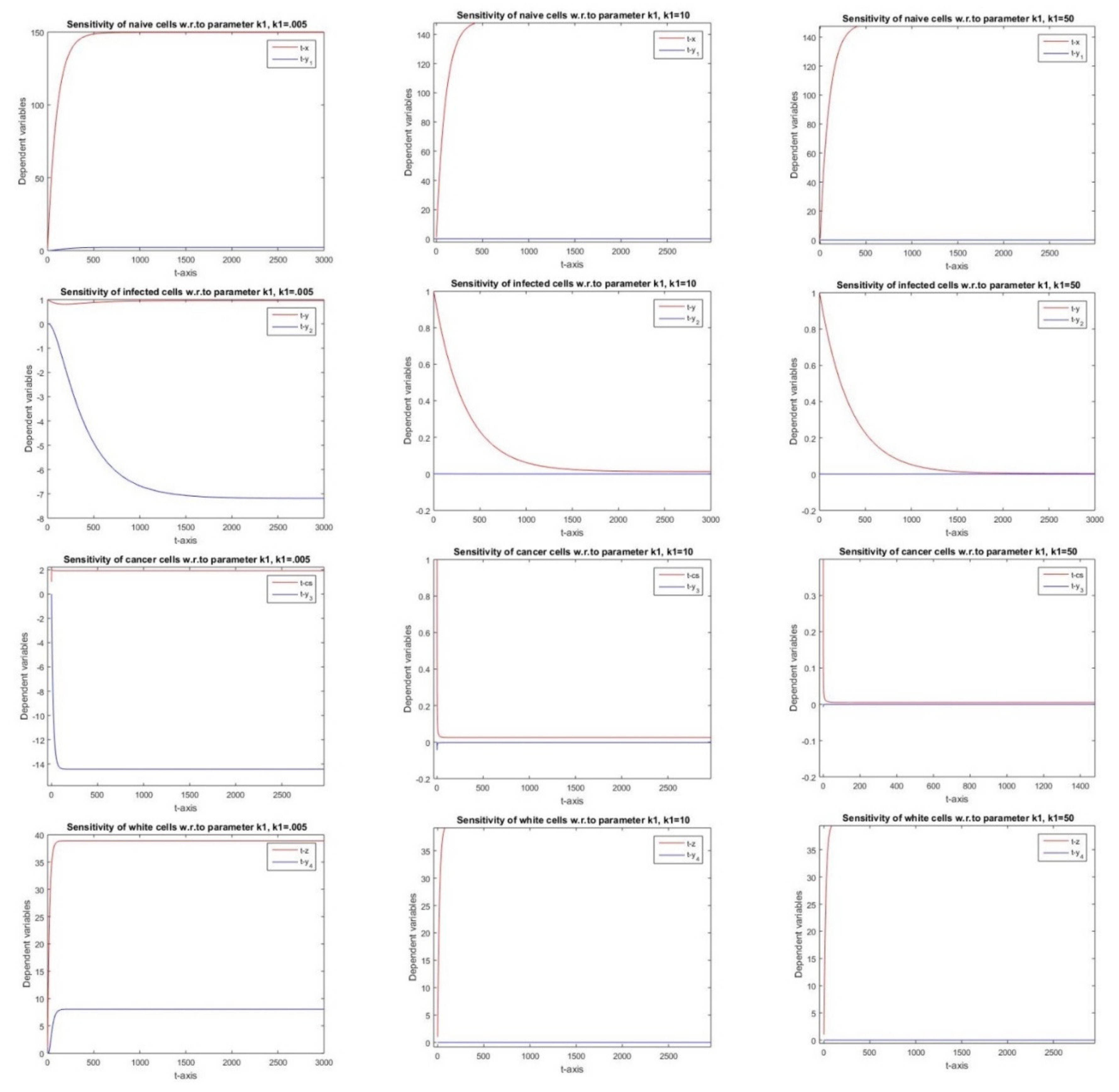
2.2.7. Sensitivity with Respect to Parameter k₁

This term $‘\frac{\partial y}{\partial k_1}’$ provides the much-needed sensitivity equations.

We define

$$y_1=\frac{\partial x}{\partial k_1},y_2=\frac{\partial y}{\partial k_1},y_3=\frac{\partial c_s}{\partial k_1},y_4=\frac{\partial z}{\partial k_1}$$

$$\begin{array}{c}{\dot{y}}_1\left(t\right)=-a_0{y}_1-\beta x{y}_3-\beta c_s{y}_1\hfill \\ {\dot{y}}_2\left(t\right)=\beta x{y}_3+\beta c_s{y}_1-{\beta }_0{y}_2\hfill \\ {\dot{y}}_3\left(t\right)=-k_0{y}_3-c_{s}z-k_1{c}_s{y}_4-k_{1}z{y}_3\hfill \\ {\dot{y}}_4\left(t\right)=b{y}_3-b_0{y}_4-b_1{c}_s{y}_4-b_{1}z{y}_3\hfill \end{array}$$

(9)

Equation $\left(9\right)$ shows the sensitivity expression with respect to parameter ‘k₁’.

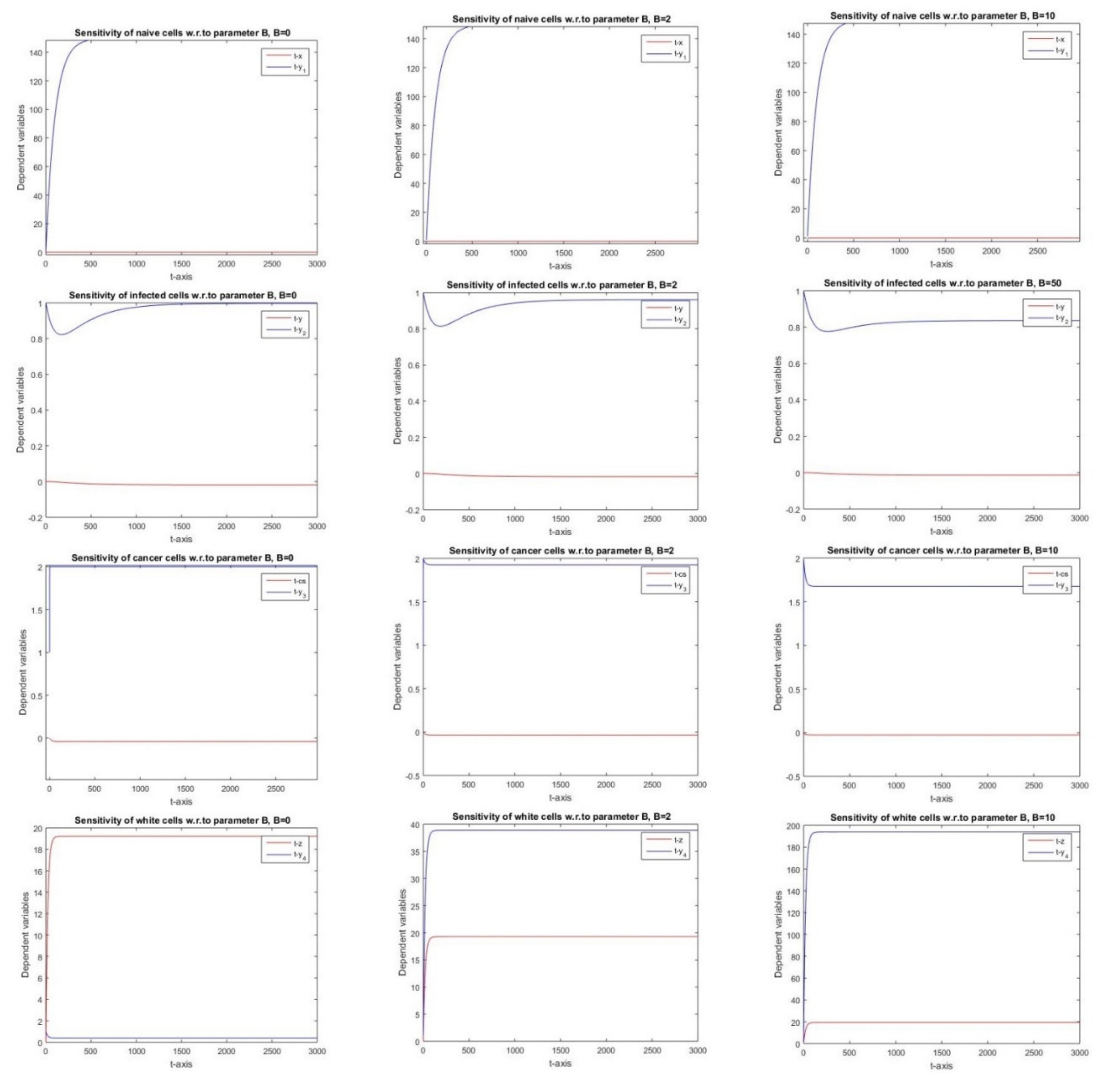
2.2.8. Sensitivity with Respect to Parameter B

This term $‘\frac{\partial y}{\partial B}’$ provides the much-needed sensitivity equations.

We define

$$y_1=\frac{\partial x}{\partial B},y_2=\frac{\partial y}{\partial B},y_3=\frac{\partial c_s}{\partial B},y_4=\frac{\partial z}{\partial B}$$

$$\begin{array}{c}{\dot{y}}_1\left(t\right)=-a_0{y}_1-\beta x{y}_3-\beta c_s{y}_1\hfill \\ {\dot{y}}_2\left(t\right)=\beta x{y}_3+\beta c_s{y}_1-{\beta }_0{y}_2\hfill \\ {\dot{y}}_3\left(t\right)=-k_0{y}_3-k_1{c}_s{y}_4-k_{1}z{y}_3\hfill \\ {\dot{y}}_4\left(t\right)=1+b{y}_3-b_0{y}_4-b_1{c}_s{y}_4-b_{1}z{y}_3\hfill \end{array}$$

(10)

Equation $\left(10\right)$ shows the sensitivity expression with respect to parameter ‘B’.

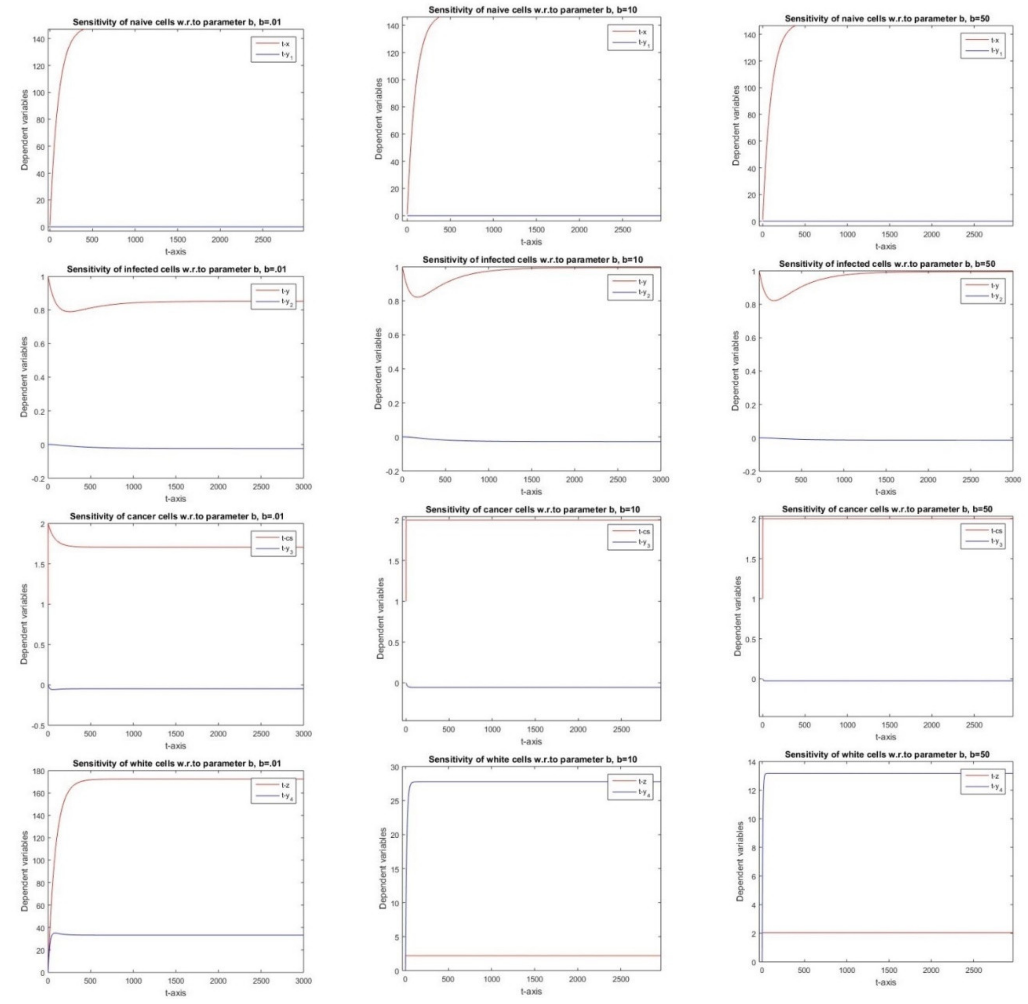
2.2.9. Sensitivity with Respect to Parameter b

This term $‘\frac{\partial y}{\partial b}’$ provides the much-needed sensitivity equations.

We define

$$y_1=\frac{\partial x}{\partial b},y_2=\frac{\partial y}{\partial b},y_3=\frac{\partial c_s}{\partial b},y_4=\frac{\partial z}{\partial b}$$

$$\begin{array}{c}{\dot{y}}_1\left(t\right)=-a_0{y}_1-\beta x{y}_3-\beta c_s{y}_1\hfill \\ {\dot{y}}_2\left(t\right)=\beta x{y}_3+\beta c_s{y}_1-{\beta }_0{y}_2\hfill \\ {\dot{y}}_3\left(t\right)=-k_0{y}_3-k_1{c}_s{y}_4-k_{1}z{y}_3\hfill \\ {\dot{y}}_4\left(t\right)=b{y}_3+c_s-b_0{y}_4-b_1{c}_s{y}_4-b_{1}z{y}_3\hfill \end{array}$$

(11)

Equation $\left(11\right)$ shows the sensitivity expression with respect to parameter ‘b’.

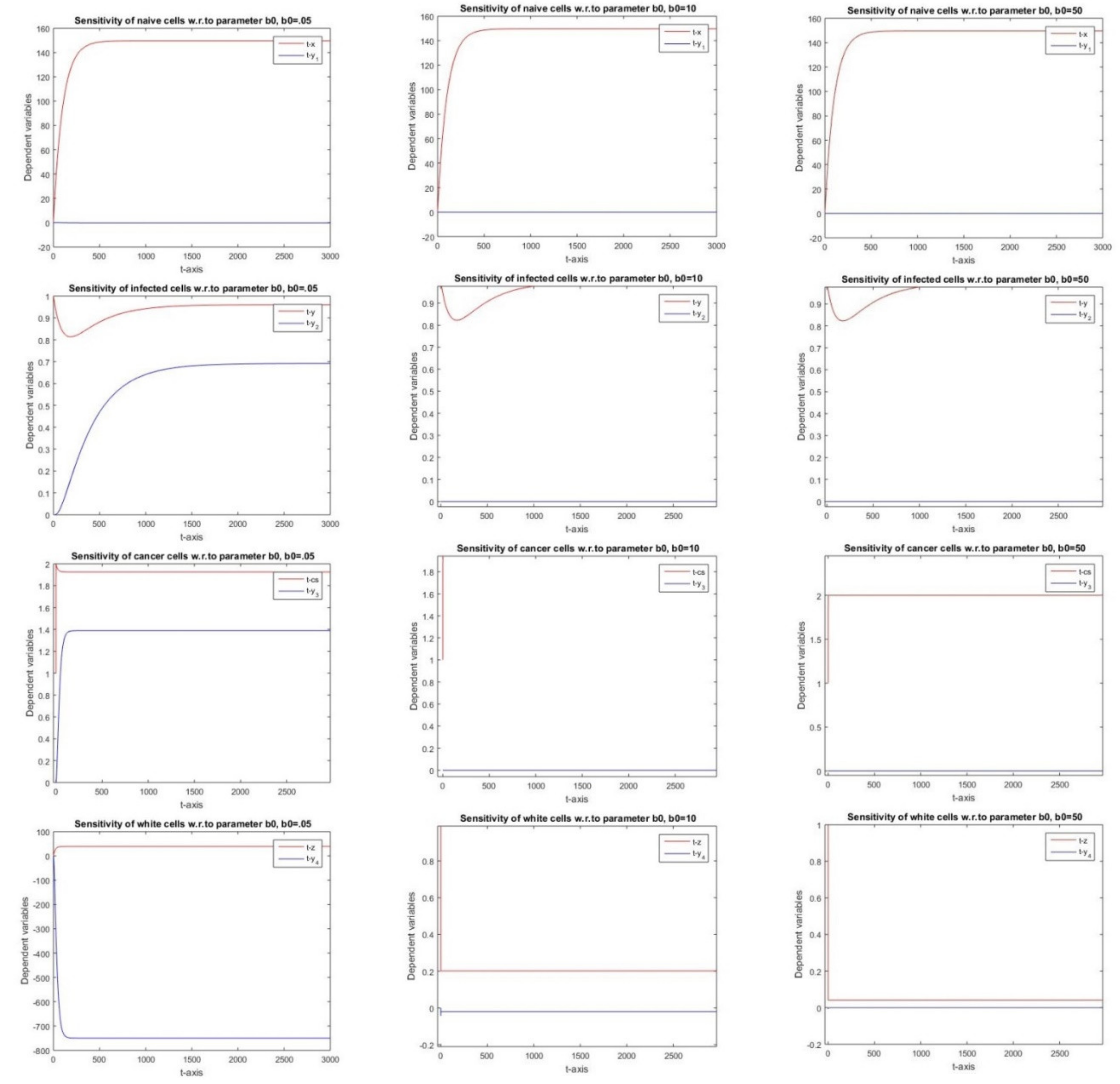
2.2.10. Sensitivity Analysis w.r.ro Parameter b₀

This term $‘\frac{\partial y}{\partial b_0}’$ provides the much-needed sensitivity equations.

We define

$$y_1=\frac{\partial x}{\partial b_0},y_2=\frac{\partial y}{\partial b_0},y_3=\frac{\partial c_s}{\partial b_0},y_4=\frac{\partial z}{\partial b_0}$$

$$\begin{array}{c}{\dot{y}}_1\left(t\right)=-a_0{y}_1-\beta x{y}_3-\beta c_s{y}_1\hfill \\ {\dot{y}}_2\left(t\right)=\beta x{y}_3+\beta c_s{y}_1-{\beta }_0{y}_2\hfill \\ {\dot{y}}_3\left(t\right)=-k_0{y}_3-k_1{c}_s{y}_4-k_{1}z{y}_3\hfill \\ {\dot{y}}_4\left(t\right)=b{y}_3-b_0{y}_4-z-b_1{c}_s{y}_4-b_{1}z{y}_3\hfill \end{array}$$

(12)

Equation $\left(12\right)$ shows the sensitivity expression with respect to parameter ‘b₀’.

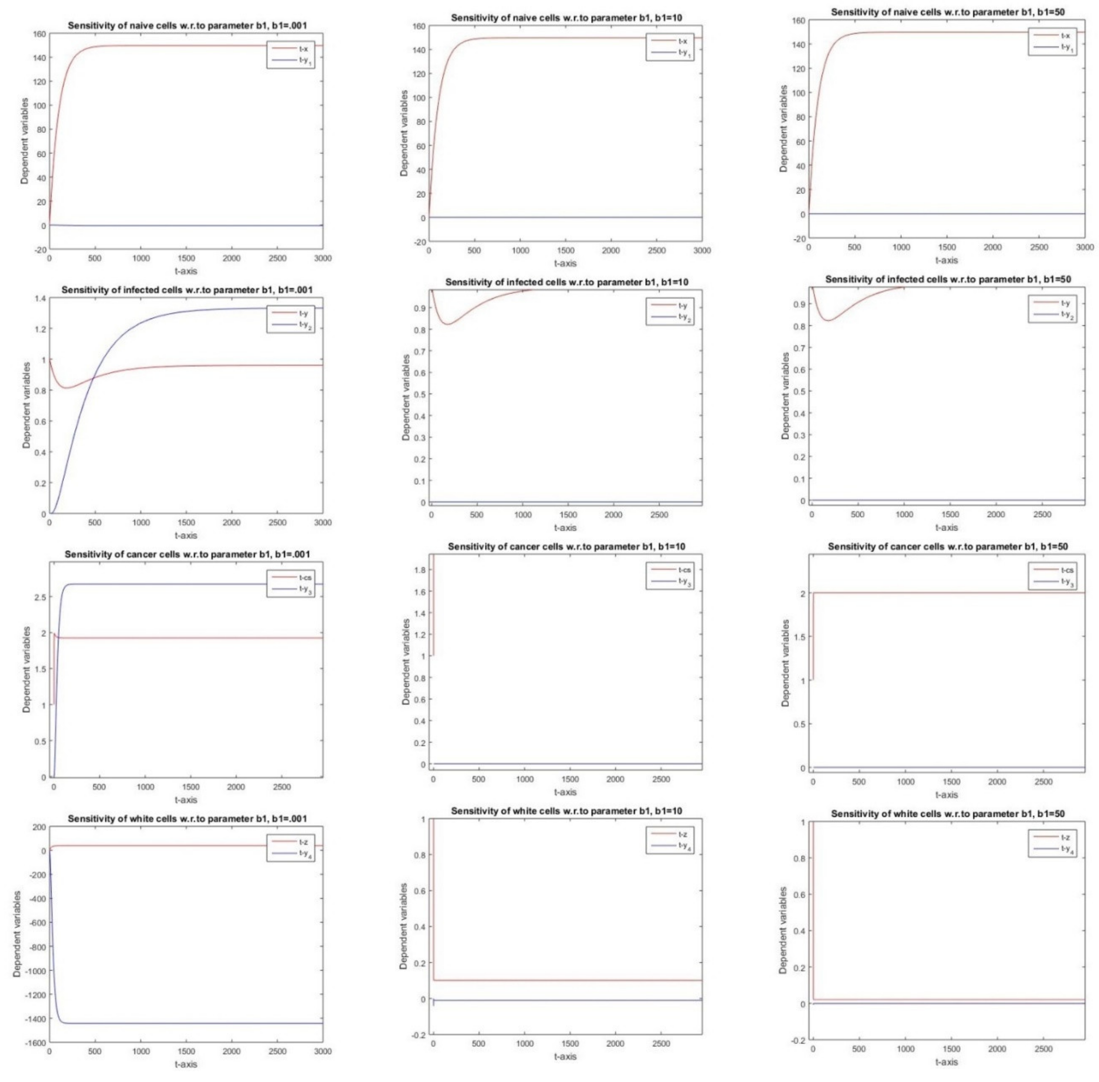
2.2.11. Sensitivity Analysis w.r.ro Parameter b₁

This term $‘\frac{\partial y}{\partial b_1}’$ provides the much-needed sensitivity equations.

We define

$$y_1=\frac{\partial x}{\partial b_1},y_2=\frac{\partial y}{\partial b_1},y_3=\frac{\partial c_s}{\partial b_1},y_4=\frac{\partial z}{\partial b_1}$$

$$\begin{array}{c}{\dot{y}}_1\left(t\right)=-a_0{y}_1-\beta x{y}_3-\beta c_s{y}_1\hfill \\ {\dot{y}}_2\left(t\right)=\beta x{y}_3+\beta c_s{y}_1-{\beta }_0{y}_2\hfill \\ {\dot{y}}_3\left(t\right)=-k_0{y}_3-k_1{c}_s{y}_4-k_{1}z{y}_3\hfill \\ {\dot{y}}_4\left(t\right)=b{y}_3-b_0{y}_4-z{c}_s-b_1{c}_s{y}_4-b_{1}z{y}_3\hfill \end{array}$$

(13)

Equation $\left(13\right)$ shows the sensitivity expression with respect to parameter ‘b₁’.

3. Results

Here, we justify our sensitivity equations numerically by opting the nominal values for the parameters under consideration for sensitivity. The chosen nominal values are as follows.

$$\begin{array}{l}A=1.5,a_0=0.01,\beta =0.00001,{\beta }_0=0.003,k=10,k_0=5,\\ k_1=0.005,B=2,b=0.01,b_0=0.05,b_1=0.001\end{array}$$

We assumed nominal values for the initial condition of the differential equations system. We carried out numerical simulations using MATLAB [27].

With the help of MATLAB, we produced graphical results of the sensitivity equations that we obtained from the application of the definition of sensitivity. Since the results obtained were in analytical form, to facilitate the reader’s understanding of their meaning, the parameter sensitivity results are drawn in the form of graphs.

3.1. Parameter A

As we increase the recruitment rate of naïve cells, it is observed in Figure 1 that the population of naïve and infected blood cells increases abruptly, and then abruptly decreases in both the populations and, with further increase, there is no change. This is because, with the increase in the recruitment rate of naïve cells, naïve cells increase in number then, because of their death rate and interaction with cancer cells, their population decreases. A similar pattern is followed by infected cells because of their death rate, and the availability of less susceptible cells that become infected in the long run. No change is observed in cancer and immune cells because there is no interaction of these populations with the rest.

3.2. Parameter a₀

As we increase the value of ‘a₀’, which shows the natural death rate of naïve cells, an initially abrupt change is observed in the naïve and infected cells’ population as seen in Figure 2. Both the populations decrease abruptly and, when this rate is further increased, a negligible decrease is observed in both populations and no change is observed, further increasing their natural death rate. The rest of the two populations remain unchanged, as is obvious from mathematical model as well as from the sensitivity equations.

3.3. Parameter β

As seen in Figure 3, all the populations remain unchanged as we increase the decay rate of naïve cells. This is because, upon the interaction of these two populations, i.e., naïve and cancer cells, naïve cells are either killed or become dysfunctional and, since the dysfunctional cells become part of the infected cells’ population, they further disappear because of their natural death rate. Because of this fact, there remains a balance in both populations, and hence no change is observed. The rest of the two populations also remains unchanged because of their lack of connection with the previous populations.

3.4. Parameter β₀

Since ‘β₀’ represents the natural death rate and is associated with the infected cells, there is an abrupt decrease in the infected populace, as an increased number of infected cells becomes available as shown in Figure 4, and then, because of their natural death rate, the population lessens with a negligibly small change, and with a further increase at this rate, no change is observed under the study of dysfunctional cells.

3.5. Parameter k

As far as the behavior of ‘k’ is concerned, we notice in Figure 5 that, as the value of ‘k’, i.e., the recruitment rate of cancer cells is increased, an abrupt increase in the number of infected and cancer cells is observed. However, as the value is increased further, then, because of the already high population of cancer cells, there is a saturation level for this population and, due to an increased death rate and high number of encounters with immune cell, there is no further increase in infected and cancer population, and behavior is somewhat stable in the long run. The other population remains invariant.

3.6. Parameter k₀

It can be seen from Figure 6 that a noticeable decrease occurs in the population of infected and cancer cells as the natural death rate is increased. The decay of these populations is much faster because of the high population and, with the passage of time, there is a lower population and change occurs negligibly. Finally, a stage comes when there are no more infected and cancer cells.

3.7. Parameter k₁

It can be seen in Figure 7 that there is an abrupt decrease in the number of infected and cancer cells. This noticeable change occurs with respect to the increase in the coefficient ‘k₁’, whereas, at the same time, there is abrupt increase in the number of immune cells. After a short time period, the numbers reach the steady state.

3.8. Parameter B

When there is no external re-infusion of T cells, the number of available infected and cancer cells is higher and there are less immune cells. As we increase the external re-infusion of T cells into cancer patients, the amount of infected and cancer cell decreases and a relative increase in the amount of immune cells is observed as shown in Figure 8.

3.9. Parameter b

Since ‘b’ is the proliferation rate of T cells due to cancer antigen-presenting cells in the blood of cancer relapse patients, this term behaves similarly to the external re-infusion and similar behavior is observed graphically in Figure 9.

3.10. Parameter b₀

As we increase the death rate of immune cells, it is observed in Figure 10 that, initially, there is an abrupt decrease in the amount of immune cells and, due to this, an abrupt increase in infected and cancer cells. However, as we go on increasing its death rate then, due to the lack of immune cells present in the body because of the higher death rate and their being killed by cancer cells, the change in the population of immune cells is almost negligible and, finally, there comes a stage when there is an absence of immune cells, and hence no further change is observed in the population of immune cells as well as cancer and infected cells, because there is no interaction between cancer and immune cells. However, the population of susceptible cells remains unchanged.

3.11. Parameter b₁

As ‘b₁’ is the loss rate of immune cells due to encounters with cancer cells, similar behavior is observed in Figure 11 as that observed in the case of ‘b₀’.

4. Conclusions

In this paper, we considered a mathematical model developed for studying the effect of genetically engineered T cells on the spread of Leukemia. The model is directed by four non-linear ordinary differential equations. The model is investigated for sensitivity purposes analytically as well as numerically.

Analytically, we applied a very basic approach to compute the sensitivity of each parameter in a local sense by taking the partial derivative of all dependent variables with respect to the parameters whose sensitivity is to be determined, by varying only that parameter while keeping others fixed. Since we received a large amount of reliable information from the numerical approach, we applied a numerical approach using the sensitivity equations obtained from the analytical approach, and plotted a graph to provide visual insight, as discussed in [28].

The sensitivity analysis justified the use of immunotherapy. All the parameters are sensitive, but some of them are identified as having negligible effect on the system. The most important parameter found in controlling leukemia is the transfusion of genetically engineered T cells, as this showed a noticeable decrease in infected and cancer cells, which was the key purpose of this paper. One of the edges of this parameter is that it produces a dormant memory, which, in turn, helps to fight leukemia in case of relapse.

The conclusions obtained after applying a sensitivity analysis from a numerical approach graphically suggest that immunotherapy with T cell infusion is better than other techniques available for treatment as it has less harmful effects to the body, and the dormant memory of immune cells to fight leukemia is extremely beneficial.

Last but not least, sensitivity analysis provides insight into the operational principles of the system, providing an opportunity for mathematicians to improve it and help improve treatment.

References

1. Gross, L.J. Points of View: The Interface of Mathematics and Biology. Cell Biol. Educ. 2004, 3, 85–87. [Google Scholar] [CrossRef] [PubMed]
2. Elango, P. The Role of Mathematics in Biology; South Eastern University of Sri Lanka: Oluvil, Sri Lanka, 2015. [Google Scholar]
3. Dreij, K.; Chaudhry, Q.A.; Jernström, B.; Morgenstern, R.; Hanke, M. A method for efficient calculation of diffusion and reactions of lipophilic compounds in complex cell geometry. PLoS ONE 2011, 6, e23128. [Google Scholar] [CrossRef] [PubMed] [Green Version]
4. Riaz, S.; Chaudhry, Q.A.; Siddiqui, S. Mathematical modeling and optimization of complex structures: A review. Complex Adapt. Syst. Modeling 2016, 4, 1–3. [Google Scholar] [CrossRef] [Green Version]
5. Khalid, S.; Chaudhry, Q.A. Quantitative analysis of cancer risk assessment in a mammalian cell with the inclusion of mitochondria. Comput. Math. Appl. 2019. [Google Scholar] [CrossRef]
6. Chaudhry, Q.A.; Hanke, M.; Morgenstern, R.; Dreij, K. Surface reactions on the cytoplasmatic membranes—Mathematical modeling of reaction and diffusion systems in a cell. J. Comput. Appl. Math. 2014, 262, 244–260. [Google Scholar] [CrossRef]
7. Dreij, K.; Chaudhry, Q.A.; Jernström, B.; Hanke, M.; Morgenstern, R. In silico modeling of intracellular diffusion and reaction of benzo. Pyrene Diol Epoxide 2012, 211, S60–S61. [Google Scholar]
8. Felman, A. What to Know about Leukemia. Available online: https://www.medicalnewstoday.com/articles/142595 (accessed on 10 January 2020).
9. Marieb, E.N.; Hoehn, K.N. Human Anatomy & Physiology; Pearson Education: London, UK, 2015. [Google Scholar]
10. Martini, F.H.; Nath, J.L.; Bartholomew, E.F. Fundamentals of Anatomy & Physiology; Global Edition; Pearson: London, UK, 2018. [Google Scholar]
11. MacGill, M. What Does the Lymphatic System Do? Available online: https://www.medicalnewstoday.com/articles/303087 (accessed on 10 January 2020).
12. Gray, H.; Lewis, W.H. Anatomy of the Human Body; Lea & Febiger: Philadelphia, PA, USA, 1918. [Google Scholar]
13. Lim, H.; Yeo, K.; Angeli, V. Lipid biology and lymphatic function: A dynamic interplay with important physiological and pathological consequences. J. Clin. Cell Immunol. 2014, 5, 2. [Google Scholar]
14. Bertuccio, P.; Bosetti, C.; Malvezzi, M.; Levi, F.; Chatenoud, L.; Negri, E.; Vecchia, C.L. Trends in mortality from leukemia in Europe: An update to 2009 and a projection to 2012. Int. J. Cancer 2013, 132, 427–436. [Google Scholar] [CrossRef] [PubMed]
15. Fitzmaurice, C.; Allen, C.; Barber, R.M.; Barregard, L.; Bhutta, Z.A.; Brenner, H.; Dicker, D.J.; Chimed-Orchir, O.; Dandona, R.; Dandona, L. Global, regional, and national cancer incidence, mortality, years of life lost, years lived with disability, and disability-adjusted life-years for 32 cancer groups, 1990 to 2015: A systematic analysis for the global burden of disease study. JAMA Oncol. 2017, 3, 524–548. [Google Scholar] [PubMed]
16. Combest, A.J.; Danford, R.C.; Andrews, E.R.; Simmons, A.; Mcatee, P.; Reitsma, D.J. Overview of the Current Treatment Paradigm in Chronic Lymphocytic Leukemia, Part 2. J. Hematol. Oncol. Pharm. 2016, 6, 89–94. [Google Scholar]
17. Hus, I.; Roliński, J. Current concepts in diagnosis and treatment of chronic lymphocytic leukemia. Contemp. Oncol. 2015, 19, 361. [Google Scholar] [CrossRef] [PubMed] [Green Version]
18. Lu, K.; Wang, X. Therapeutic advancement of chronic lymphocytic leukemia. J. Hematol. Oncol. 2012, 5, 55. [Google Scholar] [CrossRef] [PubMed] [Green Version]
19. Scheithauer, H.; Belka, C.; Lauber, K.; Gaipl, U.S. Immunological Aspects of Radiotherapy; Springer: Berlin, Germany, 2014. [Google Scholar]
20. Watanabe, Y.; Dahlman, E.L.; Leder, K.Z.; Hui, S.K. A mathematical model of tumor growth and its response to single irradiation. Theor. Biol. Med. Model. 2016, 13, 6. [Google Scholar] [CrossRef] [PubMed] [Green Version]
21. Gatza, E.; Wahl, D.R.; Opipari, A.W.; Sundberg, T.B.; Reddy, P.; Liu, C.; Glick, G.D.; Ferrara, J.L. Manipulating the bioenergetics of alloreactive T cells causes their selective apoptosis and arrests graft-versus-host disease. Sci. Transl. Med. 2011, 3, ra67–ra68. [Google Scholar] [CrossRef] [PubMed] [Green Version]
22. Agur, Z.; Vuk-Pavlović, S. Mathematical modeling in immunotherapy of cancer: Personalizing clinical trials. Mol. Ther. 2012, 20, 1–2. [Google Scholar] [CrossRef] [PubMed] [Green Version]
23. Agarwal, M.; Bhadauria, A.S. Mathematical Modeling and Analysis of Leukemia: Effect of External Engineered T Cells Infusion. Appl. Appl. Math. 2015, 10, 249–266. [Google Scholar]
24. Saltelli, A. Sensitivity Analysis. 2017. Available online: http://www.andreasaltelli.eu/file/repository/Bergen_Andrea_Thursday_SA.pdf (accessed on 10 January 2020).
25. Zi, Z. Sensitivity analysis approaches applied to systems biology models. IET Syst. Biol. 2011, 5, 336–346. [Google Scholar] [CrossRef] [PubMed]
26. Huang, Q. Sensitivity Analysis in Biological Modelling. 2012. Available online: http://www.math.ualberta.ca/~hwang/sensitivity (accessed on 10 January 2020).
27. Davis, T.A. MATLAB Primer, 8th ed.; CRC Press: Boca Raton, FL, USA, 2011. [Google Scholar]
28. Bolboacă, S.D. Medical Diagnostic Tests: A Review of Test Anatomy, Phases, and Statistical Treatment of Data. Comput. Math. Methods Med. 2019. [Google Scholar] [CrossRef] [PubMed] [Green Version]
Figure 1. Graphs of sensitivity with respect to A: Row 1 represents the sensitivity of naïve cells with respect to the change in A; Row 2 shows the sensitivity of Infected Cells; Row 3 shows the sensitivity of cancer cells, whereas Row 4 represents the sensitivity of white cells. In each case, sensitivity was observed with variations in A by taking the value to be 1.5, 10 and 50.
Mathematics 08 00564 g001
Figure 2. Graphs of sensitivity with respect to a0: Row 1 represents the sensitivity of naïve cells with respect to the change in a0; Row 2 shows the sensitivity of infected cells; Row 3 shows the sensitivity of cancer cells, whereas Row 4 represents the sensitivity of white cells. In each case, sensitivity was observed with variations in a0 by taking the value to be 0.01, 10 and 50.
Mathematics 08 00564 g002
Figure 3. Graphs of sensitivity with respect to β: Row 1 represents the sensitivity of naïve cells with respect to the change in β; Row 2 shows the sensitivity of infected cells; Row 3 shows the sensitivity of cancer cells, whereas Row 4 represents the sensitivity of white cells. In each case, sensitivity was observed with variations in β by taking the values to be 0.00001, 10 and 50.
Mathematics 08 00564 g003
Figure 4. Graphs of sensitivity with respect to β0: Row 1 represents the sensitivity of naïve cells with respect to the change in β0; Row 2 shows the sensitivity of infected cells; Row 3 shows the sensitivity of cancer cells, whereas Row 4 represents the sensitivity of white cells. In each case, sensitivity was observed with variations in β0 by taking the value to be 0.003, 10 and 50.
Mathematics 08 00564 g004
Figure 5. Graphs of sensitivity with respect to k: Row 1 represents the sensitivity of naïve cells with respect to the change in k; Row 2 shows the sensitivity of infected cells; Row 3 shows the sensitivity of cancer cells, whereas Row 4 represents the sensitivity of white cells. In each case, sensitivity was observed with variations in k by taking the value to be 1, 10 and 50.
Mathematics 08 00564 g005
Figure 6. Graphs of sensitivity with respect to k0: Row 1 represents the sensitivity of naïve cells with respect to the change in k0; Row 2 shows the sensitivity of infected cells; Row 3 shows the sensitivity of cancer cells, whereas Row 4 represents the sensitivity of white cells. In each case, sensitivity was observed with variations in k0 by taking the value to be 5, 10 and 50.
Mathematics 08 00564 g006
Figure 7. Graphs of sensitivity with respect to k1: Row 1 represents the sensitivity of naïve cells with respect to the change in k1; Row 2 shows the sensitivity of infected cells; Row 3 shows the sensitivity of cancer cells, whereas Row 4 represents the sensitivity of white cells. In each case, sensitivity was observed with variations in k1 by taking the value to be 0.005, 10 and 50.
Mathematics 08 00564 g007
Figure 8. Graphs of sensitivity with respect to B: Row 1 represents the sensitivity of naïve cells with respect to the change in B; Row 2 shows the sensitivity of infected cells; Row 3 shows the sensitivity of cancer cells, whereas Row 4 represents the sensitivity of white cells. In each case, sensitivity was observed with variations in B by taking the value to be 0, 2 and 10.
Mathematics 08 00564 g008
Figure 9. Graphs of sensitivity with respect to b: Row 1 represents the sensitivity of naïve cells with respect to the change in b; Row 2 shows the sensitivity of infected cells; Row 3 shows the sensitivity of cancer cells, whereas Row 4 represents the sensitivity of white cells. In each case, sensitivity was observed with variations in b by taking the value to be 0.01, 10 and 50.
Mathematics 08 00564 g009
Figure 10. Graphs of sensitivity with respect to b0: Row 1 represents the sensitivity of naïve cells with respect to the change in b0; Row 2 shows the sensitivity of infected cells; Row 3 shows the sensitivity of cancer cells, whereas Row 4 represents the sensitivity of white cells. In each case, sensitivity was observed with variations in b0 by taking the value to be 0.05, 10 and 50.
Mathematics 08 00564 g010
Figure 11. Graphs of sensitivity with respect to b1: Row 1 represents the sensitivity of naïve cells with respect to the change in b1; Row 2 shows the sensitivity of infected cells; Row 3 shows the sensitivity of cancer cells, whereas Row 4 represents the sensitivity of white cells. In each case, sensitivity was observed with variations in b1 by taking the value to be 0.001, 10 and 50.
Mathematics 08 00564 g011