Re-Evaluating the Classical Falling Body Problem

Abstract

This paper re-analyzes the falling body problem in three dimensions, taking into account the effect of the Earth’s rotation (ER). Accordingly, the analytic solution of the three-dimensional model is obtained. Since the ER is quite slow, the three coupled differential equations of motion are usually approximated by neglecting all high order terms. Furthermore, the theoretical aspects describing the nature of the falling point in the rotating frame and the original inertial frame are proved. The theoretical and numerical results are illustrated and discussed.

1. Introduction

In recent years, the classical falling body problem (FBP) and the two-dimensional projectile motion [1,2,3,4,5,6,7,8,9,10,11] have been re-evaluated. The FBP has been modeled as the vertical motion of a particle near to the Earth’s gravitational field [12,13,14]; that is, as a problem formulated in one dimension. Hence, the results obtained in [12,13,14] are only valid in a fixed non-rotating frame. Thus, the effect of Earth’s rotation (ER) on the FBP and on the projectile motion, was not taken into account. This paper addresses such effect of the ER by analyzing the three-dimensional model of a falling body under the action of the Earth’s gravitational field.

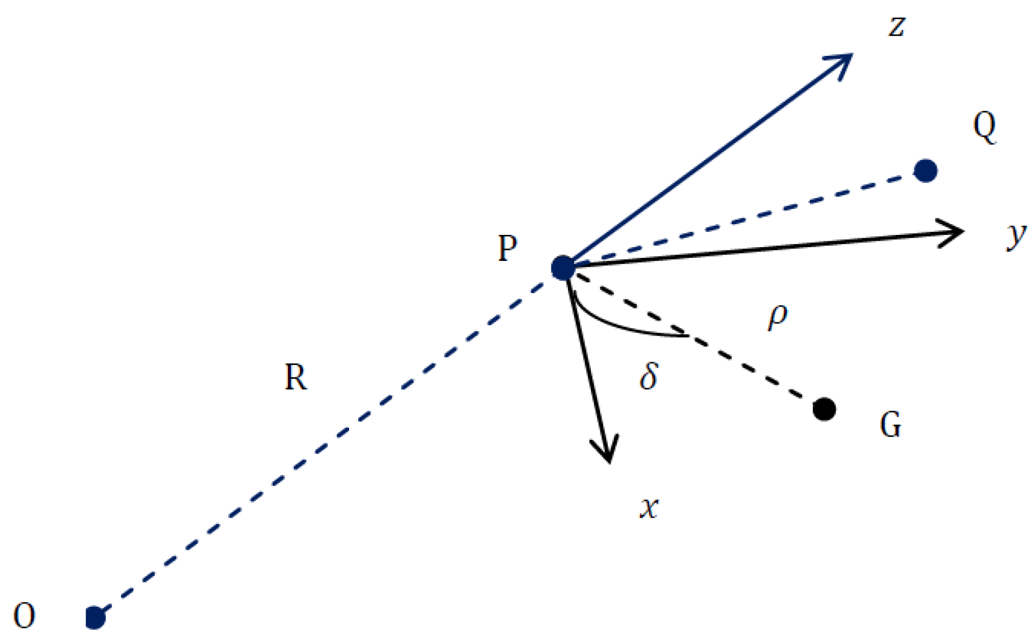
For a clear description of the problem, let us suppose that $\overrightarrow{r}=\left(x\left(t\right),y\left(t\right),z\left(t\right)\right)$ is the vector of Q near the Earth surface, relative to the surface point P; see Figure 1. The governing equations are given by [15,16]:

$$x{}^{″}\left(t\right)=\left(2\omega \cos \lambda \right)y^{\prime }\left(t\right)+{\omega }^2\left(x\left(t\right)cos\lambda +\left(R+z\left(t\right)\right)sin\lambda \right)cos\lambda ,$$

(1)

$$y{}^{″}\left(t\right)=-\left(2\omega \cos \lambda \right)x^{\prime }\left(t\right)-\left(2\omega \sin \lambda \right)z^{\prime }\left(t\right)+{\omega }^{2}y\left(t\right),$$

(2)

$$z{}^{″}\left(t\right)=-g+\left(2\omega \sin \lambda \right)y^{\prime }\left(t\right)+{\omega }^2\left(x\left(t\right)cos\lambda +\left(R+z\left(t\right)\right)sin\lambda \right)sin\lambda ,$$

(3)

where g represents the acceleration due to gravity, $\omega$ denotes the Earth’s angular velocity, $\lambda \in [0,\pi ]$ is the colatitude, and R stands for the Earth’s radius. Here, the x-, y-, and z- directions points to south, east, and up, respectively. For analysing the effects of the ER on the FBP we assume that a particle is released from rest at the point Q $=(x_0,y_0,z_0)$ under the Earth’s gravitational field. Accordingly, the initial conditions (ICs) are defined as

$$\begin{array}{c}\hfill x\left(0\right)=x_0,y\left(0\right)=y_0,z\left(0\right)=z_0,\\ \hfill x^{\prime }\left(0\right)=0,y^{\prime }\left(0\right)=0,z^{\prime }\left(0\right)=0.\end{array}$$

(4)

Figure 1. The inertial/local frames are $(x,y,z)$ and $(X,Y,Z)$, respectively. The $x-,y-,$ and $z-$ directions point to the south, east, and up (away from the Earth’s surface).

The transformation between the two systems of coordinates $(x,y,z)$ and $(X,Y,Z)$ in Figure 1 is governed by [16]:

$$X=xcos\lambda cos\varphi -ysin\varphi +\left(R+z\right)sin\lambda cos\varphi ,$$

(5)

$$Y=xcos\lambda sin\varphi +ycos\varphi +\left(R+z\right)sin\lambda sin\varphi ,$$

(6)

$$Z=-xsin\lambda +\left(R+z\right)cos\lambda ,$$

(7)

where $\lambda$ and $\varphi$ are the colatitude and longitude of the surface point P, respectively, and R is the Earth’s radius as mentioned above. However, to include the ER effect, we need to set $\varphi =\omega t$ in Equations (5)–(7). Therefore, the transformation between the frames $(x,y,z)$ and $(X,Y,Z)$ after a time t is given by [16]:

$$X=xcos\lambda cos\omega t-ysin\omega t+\left(R+z\right)sin\lambda cos\omega t,$$

(8)

$$Y=xcos\lambda sin\omega t+ycos\omega t+\left(R+z\right)sin\lambda sin\omega t,$$

(9)

$$Z=-xsin\lambda +\left(R+z\right)cos\lambda .$$

(10)

In the literature [15,16], Model (1)–(4) has been solved for a special case, namely for $x_0=y_0=0$, where all terms of order superior to ${\omega }^2$ are neglected. The objective of this paper is to re-address the approach adopted in [15,16] for solving Model (1)–(4) when $x_0\ne 0$ and $y_0\ne 0$. As one should expect, in the follow-up, it will be shown that the current solutions reduce to the previous ones [15,16] when $x_0$ and $y_0$ vanish. In addition, several Lemmas are proven for the geometrical properties of the falling point in the two frames. Finally, the theoretical results will be illustrated through several numerical examples.

2. The Classical Approximate Solution

The ER is quite slow [15,16], and we find the value $\omega =7.27\times {10}^{-5}{\mathrm{s}}^{-1}$. From Equation (1), the biggest term ${\omega }^{2}Rsin\lambda cos\lambda$ reaches its maximum value 0.016 when $\lambda =\pi /4$. Also, from Equation (3), it is noted that the maximum value of the product ${\omega }^{2}R{sin}^2\lambda$ is approximately 0.03 when $\lambda =\pi /2$. At other values of $\lambda$, these products are too small, and hence, the present analysis may still be effective, even for all planets such that their realistic data satisfy ${\omega }^{2}R\ll 1$. In addition, if ${\omega }^{2}R$ approaches one, the terms of order ${\omega }^2$ and maybe other higher orders should be considered. Hence, in the classical perspective, it is sufficient, in the present paper, to work up to the first order in $\omega$. Accordingly, all terms of order ${\omega }^2$ are ignored. At this level of accuracy, as ${\omega }^2\to 0$, the equations of Motion (1)–(3) reduce to

$$x{}^{″}\left(t\right)=\left(2\omega \cos \lambda \right)y{}^{\prime }\left(t\right),$$

(11)

$$y{}^{″}\left(t\right)=-\left(2\omega \cos \lambda \right)x{}^{\prime }\left(t\right)-\left(2\omega \sin \lambda \right)z{}^{\prime }\left(t\right),$$

(12)

$$z{}^{″}\left(t\right)=-g+\left(2\omega \sin \lambda \right)y{}^{\prime }\left(t\right),$$

(13)

Integrating Equations (11) and (13) once with respect to t and implementing the IC (4), we obtain

$$x{}^{\prime }\left(t\right)=\left(2\omega cos\lambda \right)\left(y\left(t\right)-y_0\right),$$

(14)

$$z{}^{\prime }\left(t\right)=-gt+\left(2\omega sin\lambda \right)\left(y\left(t\right)-y_0\right).$$

(15)

Inserting Equations (14) and (15) into (12), we have

$$\begin{array}{cc}y{}^{″}\left(t\right)\hfill & =-\left(4{\omega }^2{\cos }^2\lambda \right)\left(y\left(t\right)-y_0\right)+\left(2\omega g\sin \lambda \right)t-\left(4{\omega }^2{\sin }^2\lambda \right)\left(y\left(t\right)-y_0\right),\hfill \\ \hfill & =\left(2\omega g\sin \lambda \right)t-4{\omega }^2\left(y\left(t\right)-y_0\right).\hfill \end{array}$$

(16)

Neglecting the term of order ${\omega }^2$ in (16), yields

$$y{}^{″}\left(t\right)=\left(2\omega g\sin \lambda \right)t.$$

(17)

Integrating Equation (17) twice with respect to t in view of the IC (4), we obtain

$$y\left(t\right)=y_0+\left(\frac{1}{3}\omega g\sin \lambda \right)t^3+\mathrm{O}\left({\omega }^2\right).$$

(18)

Substituting Equation (18) into (14) and (15) and solving the resulting differential equations, we obtain $x\left(t\right)$ and $z\left(t\right)$:

$$x\left(t\right)=x_0+\mathrm{O}\left({\omega }^2\right),$$

(19)

$$z\left(t\right)=z_0-\frac{1}{2}g{t}^2+\mathrm{O}\left({\omega }^2\right),$$

(20)

where the terms of order ${\omega }^2$ were ignored and the ICs (4) were implemented. Clearly, when $x_0=0$, $y_0=0$, we recover the solutions in the literature [15,16]. It is observed from Equation (18) that the factor $\left(\omega g\sin \lambda \right)$ is positive $\forall \lambda \in (0,\pi )$. Accordingly, the particle is drifting away towards the east.

3. Re-analysis of the FBP

Assume that the falling body, released from Q, hits the $xy$-plane at a point G; see Figure 2. Then, the time T required for the body to hit the $xy$-plane is obtained from Equation (20) as

$$T=\sqrt{\frac{2z_0}{g}}.$$

(21)

Figure 2. The particle, at rest, is released from Q in the local Cartesian $(x,y,z)$ frame and hits the $xy$- plane at a point G. The angle between PG and the x-axis is denoted by $\delta$.

The Cartesian coordinates $(x_{\mathrm{G}},y_{\mathrm{G}},z_{\mathrm{G}})$ of the point G in the local frame $(x,y,z)$ are given from Equations (18)–(20) by

$$x_{\mathrm{G}}=x_0,y_{\mathrm{G}}=y_0+\left(\frac{1}{3}\omega g\sin \lambda \right)T^3,z_{\mathrm{G}}=0,$$

(22)

where $y_{\mathrm{G}}$ is the total eastward displacement. Let us now suppose that the point G is at a distance $\rho$ from the surface point P and that the angle between the vector PG and the x-axis is denoted by $\delta$. Then, the polar coordinates $(\rho ,\delta )$ of G are

$$\begin{array}{c}\rho =\sqrt{x_{\mathrm{G}}^2+y_{\mathrm{G}}^2}=\sqrt{x_0^2+{\left[y_0+\left(\frac{1}{3}\omega g\sin \lambda \right)T^3\right]}^2},\hfill \end{array}$$

(23)

$$\begin{array}{c}\delta ={tan}^{-1}\left(\frac{y_{\mathrm{G}}}{x_{\mathrm{G}}}\right)={tan}^{-1}\left(\frac{3y_0+\left(\omega g\sin \lambda \right)T^3}{3x_0}\right),x_0\ne 0.\hfill \end{array}$$

(24)

In general, the point G does not lie on the Earth’s surface when $\rho \ne 0$ and, therefore, G is slightly above the ground in such case. It is noted from Equation (23) that $\rho \ne 0$ if, at least, one of the three quantities $x_0$, $y_0$ or $sin\lambda$ is non-zero. This issue and some other properties of the point G are discussed by the following lemmas.

Lemma 1.

If S denotes to Earth’s surface, then G ∉ S if one of the following conditions is satisfied

1. 

$x_0=0$, $y_0=0$, $\lambda \in (0,\pi )$,

2. 

$x_0=0$, $y_0\ne 0$, $\lambda \in [0,\pi ]$,

3. 

$x_0\ne 0$, $y_0=0$, $\lambda \in [0,\pi ]$,

4. 

$x_0\ne 0$, $y_0\ne 0$, $\lambda \in [0,\pi ]$.

Proof. 

It is sufficient to prove that the distance OG (from the center of Earth to the point G) is greater than the Earth’s radius R (i.e., OG $>R$). From the geometry of the problem, the triangle $△$OPG is a right angled triangle at P. Therefore, the distance OG is given by

$$\begin{array}{cc}\hfill \mathrm{OG}& =\sqrt{R^2+{\rho }^2},\hfill \\ \hfill & =R\sqrt{1+{\left(\frac{\rho }{R}\right)}^2},\hfill \\ \hfill & =R\sqrt{1+{ϵ}^2},\mathrm{where}ϵ=\frac{\rho }{R}.\hfill \end{array}$$

(25)

From Equation (23), $ϵ$ is obtained as

$$\begin{array}{c}ϵ=\frac{\rho }{R}=\sqrt{{\left(\frac{x_0}{R}\right)}^2+{\left(\frac{y_0}{R}+\frac{\omega g{T}^3\sin \lambda }{3R}\right)}^2}.\hfill \end{array}$$

(26)

It is clear from Equation (25) that OG $>R$, i.e., G ∉ S, when $ϵ\ne 0$. At $x_0=y_0=0$, we have from Equation (26) that $ϵ=\frac{\omega g{T}^3\sin \lambda }{3R}\ne 0$ for $\lambda \in (0,\pi )$. This proves the first case.

When $x_0=0$ and $y_0\ne 0$, we find that $ϵ=\frac{y_0}{R}+\frac{\omega g{T}^3\sin \lambda }{3R}\ne 0$ for $\lambda \in [0,\pi ]$, which proves the second case. The rest of the cases can also be proved following an identical procedure. □

Lemma 2.

If G belongs to the Earth’s surface, where $x_0=0$, $y_0=0$, and $\lambda \in \{0,\pi \}$, then G is located at

1. 

The North pole of Earth if $\lambda =0$,

2. 

The South pole of Earth if $\lambda =\pi$.

Proof. 

If we set $x_0=0$, $y_0=0$ and $\lambda =0$ or $\pi$ in Equation (23), then we obtain $\rho =0$, which implies that $ϵ=0$. Hence, Equation (25) leads to OG=R and, thus, G ∈ S. To specify whether G is the North or the South pole of Earth, let us calculate the Cartesian coordinates $(X_{\mathrm{G}},Y_{\mathrm{G}},Z_{\mathrm{G}})$ of G in the inertial frame $(X,Y,Z)$. At $t=T$, we have from Equations (8)–(10) that

$$X_{\mathrm{G}}=x_{\mathrm{G}}cos\lambda cos\omega T-y_{\mathrm{G}}sin\omega T+\left(R+z_{\mathrm{G}}\right)sin\lambda cos\omega T,$$

(27)

$$Y_{\mathrm{G}}=x_{\mathrm{G}}cos\lambda sin\omega T+y_{\mathrm{G}}cos\omega T+\left(R+z_{\mathrm{G}}\right)sin\lambda sin\omega T,$$

(28)

$$Z_{\mathrm{G}}=-x_{\mathrm{G}}sin\lambda +\left(R+z_{\mathrm{G}}\right)cos\lambda .$$

(29)

Substituting $x_0=y_0=0$ into Equation (22), yields

$$x_{\mathrm{G}}=0,y_{\mathrm{G}}=\left(\frac{1}{3}\omega g\sin \lambda \right)T^3,z_{\mathrm{G}}=0,$$

(30)

Inserting Equation (30) into (27)–(29), we have

$$X_{\mathrm{G}}=-\left(\frac{1}{3}\omega g\sin \lambda \right)T^{3}sin\omega T+Rsin\lambda cos\omega T,$$

(31)

$$Y_{\mathrm{G}}=\left(\frac{1}{3}\omega g\sin \lambda \right)T^{3}cos\omega T+Rsin\lambda sin\omega T,$$

(32)

$$Z_{\mathrm{G}}=Rcos\lambda .$$

(33)

At $\lambda =0$, we obtain

$$X_{\mathrm{G}}=0,Y_{\mathrm{G}}=0,Z_{\mathrm{G}}=R,$$

(34)

that are the Cartesian coordinates of the North pole in the frame $(X,Y,Z)$. Also, we have from Equations (31)–(33) at $\lambda =\pi$ that

$$X_{\mathrm{G}}=0,Y_{\mathrm{G}}=0,Z_{\mathrm{G}}=-R,$$

(35)

which are equivalent to the Cartesian coordinates of the South pole. □

4. Results and Discussion

This section presents several numerical examples illustrating the application of the previous models. Furthermore, the two Lemmas presented previously will be validated during the discussion.

Table 1 lists the values of the falling time T given by Equation (21). Moreover, the Cartesian coordinates of Equation (22) of the falling point G in the frame $(x,y,z)$ are calculated at ten different cases of the colatitude $\lambda$ and the release point Q $=(x_0,y_0,z_0)$. Table 2 gives the corresponding polar coordinates $(\rho ,\delta )$ of G and the distance OG for the ten cases considered in Table 1.

Table 1. The values of the falling time (T) [s] and the Cartesian coordinates of the falling point G in the frame $(x,y,z)$ at various values of the colatitude ($\lambda$) [Radian] and the release point Q.

Case	Colatitude ($\mathit{\lambda }$) [Radian]	Cartesian Coordinates of the Release Point Q			Falling Time (T) [s]	Cartesian Coordinates of G
		${\mathit{x}}_0$ [km]	${\mathit{y}}_0$ [km]	${\mathit{z}}_0$ [km]		${\mathit{x}}_{\mathbf{G}}$ [km]	${\mathit{y}}_{\mathbf{G}}$ [km]	${\mathit{z}}_{\mathbf{G}}$ [km]
1	0	0	0	10	45.1754	0	0	0
2	$\pi$	0	0	10	45.1754	0	0	0
3	$\pi /4$	0	0	10	45.1754	0	0.015487	0
4	$\pi /4$	10	0	10	45.1754	10	0.015487	0
5	$\pi /4$	0	10	10	45.1754	0	10.015500	0
6	$\pi /4$	10	10	10	45.1754	10	10.015500	0
7	$\pi /6$	20	20	20	63.8877	20	20.030973	0
8	$\pi /6$	30	30	30	78.2461	30	30.056902	0
9	$\pi /6$	40	40	40	90.3508	40	40.087607	0
10	$\pi /6$	50	50	50	101.015	50	50.122434	0

Table 2. The polar coordinates $(\rho ,\delta )$ of G and the distance OG from the center of Earth to the falling point G.

Case	The Distance ($\mathit{\rho }$) [km]	The Angle ($\mathit{\delta }$) [Radian]	The Distance OG [km]	Description of G
1	0	Not available	6.37800000000	$\mathrm{G}\in \mathrm{S}$
2	0	Not available	6.37800000000	$\mathrm{G}\in \mathrm{S}$
3	0.015487	1.570796	6.37800000002	$\mathrm{G}\notin \mathrm{S}$
4	10.000000	0.001549	6.37800783946	$\mathrm{G}\notin \mathrm{S}$
5	10.015500	1.570796	6.37800786374	$\mathrm{G}\notin \mathrm{S}$
6	14.153091	0.786172	6.37801570318	$\mathrm{G}\notin \mathrm{S}$
7	28.306181	0.786172	6.37806281248	$\mathrm{G}\notin \mathrm{S}$
8	42.466662	0.786346	6.37814137640	$\mathrm{G}\notin \mathrm{S}$
9	56.630524	0.786492	6.37825140742	$\mathrm{G}\notin \mathrm{S}$
10	70.797305	0.786621	6.37839292129	$\mathrm{G}\notin \mathrm{S}$

In the cases 1 and 2 of Table 1, we consider $x_0=y_0=0$, $\lambda =0$ and $\pi$, respectively. The results of such two cases show that G $=(0,0,0)$, which represents the origin of the local frame $(x,y,z)$. The corresponding value of $\rho$ is zero, as shown in Table 2, meaning that G ∈ S (i.e., G lies on the Earth’s surface), which follows Lemma 2.

Cases 3-10 occur when at least one of the values $x_0$ or $y_0$ is non-zero. We have that $\lambda \notin \{0,\pi \}$, indicating that the Cartesian coordinates of G have two zeros at most, as shown in Table 1, therefore, we get $\rho \ne 0$ for the cases 3-10 of Table 2. Consequently, we have G ∉ S, as proved by Lemma 1. In addition, the first two cases in Table 2 show that the distance OG is equal to the Earth’s radius (hence, G ∈ S) while the rest of the cases confirms that OG is greater than the Earth’s radius (thus, G ∉ S), which agrees with the results of Lemma 1.

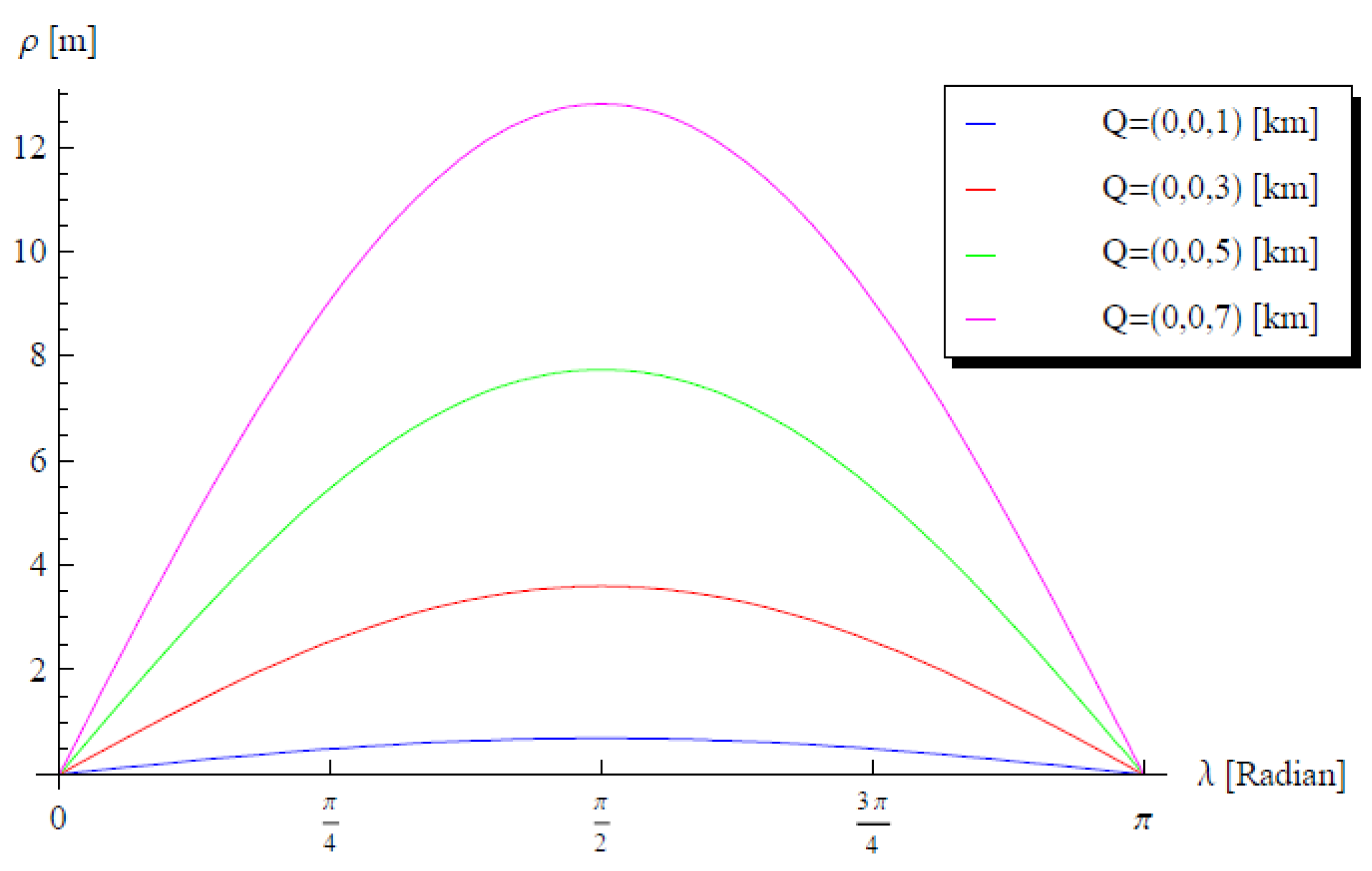
In the follow-up, it is assumed that $z_0\ne 0$ in all figures, because when $z_0=0$ we have from Equation (21) that $T=0$, which is meaningless. Figure 3 displays the variation of $\rho$ versus the colatitude $\lambda$ in the interval $[0,\pi ]$ at several release points Q $=(x_0,y_0,z_0),$ where $x_0=y_0=0$. This figure shows that the distance $\rho$ vanishes at $\lambda =0$ and $\lambda =\pi$, but we have $\rho \ne 0$ for $\lambda \in (0,\pi )$. In Figure 4, Figure 5 and Figure 6, $\rho$ is depicted against $\lambda$ at three additional cases as follows. In Figure 4, Figure 5 and Figure 6, we consider (i) $x_0=0$ and $y_0\ne 0$, (ii) $x_0\ne 0$ and $y_0=0$, and (iii) $x_0\ne 0$ and $y_0\ne 0$, respectively. From Figure 4, Figure 5 and Figure 6 It is observed that $\rho$ does not vanish for any value of $\lambda \in [0,\pi ]$. Hence, from Equation (26), we find that $ϵ\ne 0$, and therefore, Equation (25) leads to OG $>R$. This is in full agreement with the preceding Lemmas. The calculations introduced in Table 1 and Table 2, by implementing realistic data for the angular velocity and the acceleration due to gravity of Earth, are just to confirm and support the obtained theoretical Lemmas. The present results are also applicable for other planets or space bodies such that ${\omega }^{2}R\ll 1$. Moreover, it can be generalized, taking into account a resisting medium of valuable density [17].

Figure 3. Variation of $\rho$ versus the colatitude $\lambda$ at different Q $=(x_0,y_0,z_0)$ when $x_0=0,y_0=0,$ and $z_0\ne 0$.

Figure 4. Variation of $\rho$ versus the colatitude $\lambda$ at different Q $=(x_0,y_0,z_0)$ when $x_0=0,y_0\ne 0,$ and $z_0\ne 0$.

Figure 5. Variation of $\rho$ versus the colatitude $\lambda$ at different Q $=(x_0,y_0,z_0)$ when $x_0\ne 0,y_0=0,$ and $z_0\ne 0$.

Figure 6. Variation of $\rho$ versus the colatitude $\lambda$ at different Q $=(x_0,y_0,z_0)$ when $x_0\ne 0,y_0\ne 0,$ and $z_0\ne 0$.

5. Conclusions

In this paper, the three dimensional model of the FBP near to the Earth’s surface was analyzed, taking into account the ER. The analytic solutions of the three coupled equations of motion were obtained when higher orders terms of the angular velocity of Earth are neglected. The properties of the falling point in the rotating frame and the original inertial frame were given by means of two Lemmas. The conditions at which the falling point belongs to the Earth’s surface were theoretically discussed and then validated. Furthermore, the effects of the colatitude $\lambda$ and the Cartesian coordinates of the release point Q $=(x_0,y_0,z_0)$ on the final location of the falling point G $=(x_G,y_G,z_G)$ were discussed in detail. It may be helpful to refer to the limitations of the present study, which requires that ${\omega }^{2}R\ll 1$. For other planets in which ${\omega }^{2}R$ is very close to one, the terms of order ${\omega }^2$ and maybe other higher orders should be considered. In addition, if ${\omega }^{2}R\ge 1$, then all terms of $\omega$ should be taken into account, this deserves future consideration in a separate paper.