Abstract
In this paper, a stable numerical approach for recovering the membrane profile of a 2D Micro-Electric-Mechanical-Systems (MEMS) is presented. Starting from a well-known 2D nonlinear second-order differential model for electrostatic circular membrane MEMS, where the amplitude of the electrostatic field is considered proportional to the mean curvature of the membrane, a collocation procedure, based on the three-stage Lobatto formula, is derived. The convergence is studied, thus obtaining the parameters operative ranges determining the areas of applicability of the device under analysis.
1. Introduction and Problem Statement
At present, micro-components are essential in the embedded engineering applications. In particular, micro-transducers’ and micro-actuators’ results are of paramount importance due to their role of micro-devices’ interfaces [1,2]. In recent years, circular membrane MEMS technology has been exploited to this aim in a wide variety of technological fields such as thermo-elasticity [2,3,4], microfluidics [2,5,6,7], electroelasticity [8,9,10,11,12], and biomedical engineering [13,14,15]. The focus on this geometry can mainly be attributed to the availability of theoretical models in both steady-state and dynamical conditions (see [16,17,18] and references within). However, it is worth noting that these models, even though they are very detailed, are often characterized by implicit structures so that the explicit solutions are not often obtainable. As a consequence, analytical and/or algebraic conditions ensuring both existence, uniqueness, and regularity of the solution should be achieved [19], in such a way that computational results provided by numerical procedures can be checked for validating their correctness and thus avoiding possible ghost solutions. We remember that the ghost solutions are numerical solutions in convergence conditions that do not respect both analytical existence and uniqueness conditions [20,21]. On these bases, in this study, we have focused our attention on a simplified 2D circular membrane MEMS actuator in which the membrane, anchored to the edges of a fixed plate, deforms towards another fixed plate because of an applied external electrical voltage [22,23]. During the deformation of the membrane, the electrostatic field generated inside the device can be considered locally orthogonal to the membrane tangent line, so that the modulus depends (locally) on the distance between the membrane and the upper disk [19,22,23]. Accordingly, results in being proportional to the curvature of the membrane, which, being a surface in , is represented by its mean curvature (where r is the radial coordinate). The analytical model derived from these premises turns out to be a boundary value problem (BVP) with radial symmetry [22]. Precisely, it consists of a nonlinear ordinary second-order differential equation (ODE) whose independent variable is the profile of the membrane (characterized by a singularity ) with suitable conditions on both and appropriately chosen. This BVP has been studied in [22] where an algebraic condition ensuring the existence of the solution (depending on both V and the electromechanical properties of the material constituting the membrane) has been derived. Considering that the shooting procedure usually used to solve this model in some cases shows instability, in this study, we have overcome this issue by implementing a suitable collocation procedure based on the three-stage Lobatto formula [24]. Then, after a suitable rearranging of the analytical model described above, the convergence of the proposed numerical procedure has been studied. In this way, the ranges of validity of the characteristic parameters (which depend on both V and by the electromechanical properties of the material constituting the membrane) have been derived. This has made it possible to obtain, on the one hand, the avoiding of ghost solutions and, on the other hand, the identification of the area of applicability of the device, once the material constituting the membrane has been chosen (and vice versa). Furthermore, the numerical simulations have allowed for highlighting the ranges of the characteristic parameters in which instabilities of the membrane take place.
The paper is organized as follows. Section 2 reports a brief description of the membrane micro-actuator under study. Section 3 reviews some theoretical models considered as a starting point for the deduction of the model analytically studied in [22] in which . In Section 4, details on the previous points are provided. Furthermore, Section 4 shows an important result of existence, represented by an algebraic inequality. In Section 5, the applicability of the numerical procedure is demonstrated. The numerical implementation of the procedure, based on the three-stage Lobatto IIIa formula, is presented in Section 6. To facilitate the application of the numerical procedure, in Section 7, a re-elaborated version of the model is presented. In Section 8.1, the characteristic ranges of the operational parameters determining the convergence of the numerical approach are presented, while, in Section 8.2, a discussion about the instability phenomena and the ranges according to the analytical condition of uniqueness of the solution is provided. Section 8.3 makes evident the characteristic ranges of values (depending on V) ensuring both convergence and stability. In Section 9, the ghost solution areas are discussed. In Section 10, the existing links among electromechanical properties of the membrane V and the fields of applicability of the device are highlighted. Finally, in Section 11, some conclusions and future perspectives are given.
2. Electrostatic Circular MEMS Device: A Brief Description
The device under study, shown in Figure 1, is constituted by two parallel disks (both fixed), whose radius is R, and distance, d, each other. Moreover, a circular membrane, with the same radius, is clumped on the edge of the lower disk, but, when a voltage V is externally applied, it is free to deform towards the upper disk [22]. Then, is generated inside the device and, by it, an electrostatic pressure, , with permittivity of the free space, arise deflecting the membrane. In addition, the mechanical pressure p is proportional to generating a displacement at the center of the membrane, equal to , where T is the radial mechanical tension of the membrane [25]. Then, as shown in [22], that is , where k is a constant of proportionality.

Figure 1.
Representation of an electrostatic circular membrane MEMS device: the membrane is deformed towards the upper disk while the lower disk is at potential .
Remark 1.
It is worth nothing that is a very important quantity in electrostatic. In fact, the electrostatic capacitance (), co-energy function (), electrostatic charge on the membrane (q), electrostatic force (), and are dependent on . In particular, we can write (for details, see [2,22,25]):
3. Electrostatic Membrane MEMS Actuator: Some Mathematical Backgrounds
The starting point of the model studied in [22] is the well-known steady-state model largely studied in [19]. Specifically, a MEMS device consisting of two parallel metallic plates, where the lower one (at , ) is fixed and the other one (at , ), subjected to a voltage V, is deformable but anchored at their edges, is considered. The model is:
in which the existence of at least a solution has been studied exploiting Steklov boundary condition obtaining Dirichlet and Navier boundary ones. In (4), represents a bounded function that depends on the dielectric properties of the material constituting the deformable plate, and is a function depending on V. Moreover, denotes the outer normal derivative of u on . It is worth nothing that, in (4) , one obtains the Navier boundary conditions; if , one obtains the Dirichlet boundary conditions. Model (4) has been exploited in several works [3,26] in the following dimensionless version:
where L is the semi-length of the dimensionless device in order to propose a version of the model where is a parameter related to the external voltage V as follows:
in which represents the permittivity of the free space, T is the mechanical tension of the membrane, and d is ten distance between the two parallel plates. It is worth nothing that
in (6) represents the parameter that takes into account the electro-mechanical properties of the material constituting the membrane. In (5), the quantity is physically proportional to , so that it makes sense to write:
with being a parameter of proportionality. Then, in [19], since is locally orthogonal to the tangent straight line of the membrane, has been considered proportional to the curvature K of the membrane itself. Thus, taking into account that
became
with , and model (4), in [19] assumed the following form:
obtaining [19]:
in which the singularity present in (5) is not here explicitly evident. In this model, the membrane has replaced the deformable plate, and has been considered as proportional to the curvature of the membrane itself. The achieved results highlighted that the analytical uniqueness condition depended on the electro-mechanical properties of the material constituting the membrane, while the numerical solutions, obtained by a shooting procedure, highlighted the range of ensuring convergence of the procedure (without ghost solutions). Moreover, the shooting approach has been compared with the well-known Keller-box scheme getting an optimal range of (in the absence of ghost solutions).
4. A New 2D Model for Electrostatic Circular Membrane MEMS: in Terms of Mean Curvature
In [22], the attention was focused on a 2D circular membrane MEMS actuator, exploited in several biomedical and industrial applications, characterized by an axial symmetry in the geometry of the membrane. In particular, considering the z-axis as a rotation one, the profile u of the membrane has been thought as a surface generated by a vertical rotation of a curve C around z located in the first quadrant, when . In such conditions, u was only dependent on r transforming the 2D problem under study into a 1D one replacing x by r. In such a way, in (4) reduced into its radial part, so that (4) became:
in which the singularity appeared. As shown in [22], so that model (13) in [22] has been rewritten as follows:
In particular, has been supposed, for physical reasons, to be a continuous function depending on . Moreover, represented the curvature of the deformed membrane, so that
with
represented the proportionality function. Finally, model (14) became (see [22]):
where , being in 2D formulation, becomes the mean curvature. As shown in [22], the mean curvature of the membrane, , exploiting some procedures based on differential geometry concepts, can be easily written as
so that model (17) became:
from which
in which represents the critical security distance, ensuring that the deflection of the membrane does not touch the fixed upper plate. In [22], the following result of existence of at least one solution for (20) has been presented and proved as well.
Remark 2.
It is worth nothing that the mathematical models that adhere to the physical reality of MEMS are extremely complex and do not allow analytical studies on them. Therefore, it is necessary to implement some simplifications in the geometry of the MEMS device so that the simplified model obtained can be studied mathematically. It follows that the qualitative assessments obtained from the mathematical study of the model (20) (which is a simplified model) will hardly agree with any experimental data but will give (qualitative) indications of the behavior of the MEMS device characterized by simplified geometry.
Theorem 1.
Let us consider the model (20). Moreover, let and be two functions, both defined in and twice continuously differentiable, in order that . In addition:
for . Furthermore, let be a continuous function obviously, (except for ) satisfying the Generalized Lipschitz condition
where , , and are continuous functions. Moreover, . in , with . If , and
where is the permittivity of the free space and k is the constant of proportionality between the electrostatic pressure and the displacement at the center of the membrane ( ), there exists at least one solution for the problem (20).
Remark 3.
It is worth remembering that, as explained in [22], the greater k is, the lower the value of will be, so that the concavity of the membrane will rise (see (24)). However, even if (20) admits at least one solution, as specified in Theorem 1, its uniqueness has not been ensured (see Theorem 2 in [22]).
5. On the Applicability of the Numerical Procedure
As well known, the BVPs are much harder to solve than IVPs [27]. Unlike IVPs that have a unique solution, a BVP may not have a solution, or may have a finite number, or may have infinitely many. Moreover, BVPs defined on an infinite or semi-infinite interval are usual. The classical numerical approaches for solving BVPs are the shooting method and the collocation one. The first one combines a numerical method based on the solution of IVPs for ordinary differential equations (ODEs) and one for the solution of nonlinear algebraic equations. The main difficulty with the shooting method is that a perfectly well-behaved BVP can require the integration of IVPs that are not stable. This means that the solution of a BVP can be insensible to the changes in the boundary values, yet the solutions of the IVPs of shooting are sensible to the changes in the initial values. On the other side, the collocation methods are efficient and reliable tools, though, often, the underlying method may not be appropriate for high accuracies and for problems with hardly sharp changes in their solutions. The authors have used the collocation with piecewise polynomial functions and found it an appropriate method for solving the singular BVP under study because only a coefficient is singular and the solutions are smooth [27]. Then, they propose the collocation method implemented in the bvp4c routine in Matlab. The bvp4c solver is a code that implements the three-stage Lobatto IIIa formula. This is a collocation formula, and the collocation polynomial provides a continuous solution that is fourth-order accurate uniformly in the whole computational domain. Finite difference methods for BVPs are proposed in [28].
6. The Exploited Numerical Approach: A Scheme with the Three-Stage Lobatto IIIa Formula
This procedure solves a system of ODEs in the following form [24]:
where represents the boundary conditions.
Remark 4.
In this work, the authors have exploited the MatLab® R2017a bvp4c solver (Natlick, MA, USA), running on an Intel Core 2 CPU 1.45 GHz machine (Santa Clara, CA, USA) because:
- it implements a collocation technique exploiting a piecewise cubic polynomial, , whose coefficients are determined by the requirement that be continuous on ;
- the mesh and the estimation of the error are both based on the evaluation of the residual of ;
- the control of the residual is particularly useful to handle poor guesses for the mesh and the solution as well;
- the computational complexity to obtain the Jacobian is reduced;
- being a vectorized solver, it reduces the run-time vectorizing .
Let us start with the following two definitions.
Definition 1
(step-size definition). Let be the step-size computed as in the mesh-grid .
Definition 2
(midpoint & midpoint approximation). Let us denote by the midpoint of . In addition, let us indicate by the approximation of at .
Remark 5.
The cubic polynomial satisfies the boundary conditions in (25) that is . Moreover, of the mesh, the subdivision is considered, and collocates at the ends of the sub-interval and the midpoint. Obviously, is continuous at the endpoints of each sub-interval.
This collocation approach is totally equivalent to the three-stage Lobatto IIIa implicit Runge–Kutta procedure [24].
Then, after pressing the previous definitions, we are able to show the fourth-order Lobatto IIIa formula as follows:
Remark 6.
Obviously, when the procedure is applied to a quadrature problem, it reduces to the well-known Simpson formula:
Remark 7.
It is worth noting that the global discretization error of the procedure only contains even power of the step-size. This occurrence makes the method particularly attractive for both extrapolation and deferred correction.
Remark 8.
We observe that , together its derivatives, satisfies the following condition [24]:
In addition, at each intermediate point, satisfies the Equations (25) at the midpoint of each interval justifying the term “collocation polynomial”. Moreover, MatLab® chooses the form of by determining any unknown parameters. Finally:
Conditions (30)–(32) are nonlinear equations iteratively solved by a linearization procedure; then, the linear equation solver of MatLab® is used. Moreover, if necessary, the cubic polynomial can be evaluated by the bvpval function.
Remark 9.
It is worth noting that a BVP could have more than one solution so that the users should supply a guess for both the solution and the initial mesh. Then, the solver is able to adapt the mesh to achieve a solution with a reduced number of mesh points.
Obviously, a good guess is often tricky so that the solvers control the residual defined as follows.
Definition 3
(the residual). The residual in a ODE is defined as follows:
In addition, in the boundary conditions, it can be written as .
Remark 10.
We observe that, if is small, then can be considered as a good solution. In addition, if the problem is well-conditioned, small implies that is next to .
7. A More Suitable Writing of the Analytical Model
The two-point BVP under study (20) is singular with respect to the independent variable at the initial point , due to the division by zero of the first term on the right-hand side of (20). We must deal with the singularity in the coefficient at because the bvp4c solver always evaluates the ODEs at the endpoints. For this problem, we show how providing the correct value at the singular point is enough for computing the numerical solution. By the theoretical results presented in the previous sections, a smooth solution is expected. Indeed, symmetry implies that this smooth solution has a derivative that vanishes at the origin . This physical condition allows for demonstrating that
so that the singular term in the ODE is well defined at the origin for a well-behaved solution. Then, if we let in the equation, we find that
and, solving for , we obtain the value that must be used for evaluating the ODEs at the point
8. On the Convergence of the Numerical Procedure: Characteristic Ranges of and
8.1. Characteristics Ranges of
As specified above, when an external V is applied, the membrane inside the device moves towards the upper disk. The higher is the applied V, the closer the membrane to the upper disk will be. In addition, instability phenomena of the membrane can arise when V grows too much; so that it is important to know the range of V generating instability. However, V is linked to by inequality (24). Then, it follows that knowing the behavior of the membrane when increases gives us, once both and k are fixed, the range of V producing instability of the membrane in absence/presence of ghost solutions.
Remark 11.
It is interesting to observe that , being dependent on both the electromechanical properties of the material constituting the membrane and V, once the ranges of stability/instability of the membrane are known, it is possible to know the operation parameters in convergence area respecting (24) and the engineering areas of applicability of the device.
Here, it is reasonable to set . In other words, we consider that and p are totally equivalent. This makes sense because, when V is externally applied, and are generated inside the device. If we suppose that the losses are negligible, then (that is, ). Moreover, we set because lower values of do not make sense from a physical point of view. The numerical procedure has been applied for different values of and and as initial guesses. All the simulations have been carried out by bvp4c MatLab® solver on an Intel Core 2 CPU 1.45 GHz machine, using both the default relative and absolute error tolerances. Moreover, the optimal number of grid points, on the computational domain , has results of 100. In fact, by a greater number of grid points, the performance of the numerical procedure, qualitatively did not improve. Moreover, by numerical experiments, we obtain different solutions starting by different initial guesses.
The following three cases hold:
- the numerical procedure converges, and no problem arises, and instabilities do not occur. In other words, when increases starting from , in (20) increases more and more (from negative values towards zero), so that the concavity of the deformed membrane more and more decreases avoiding instabilities next to the edge of the membrane. This is confirmed by the condition (24), which ensures the existence of the solution for (20). In fact, from (24), the higher is, the lower will be; that is, increasing , the membrane does not deform too much as if a low external V is applied. Figure 2 displays an example of recovering of the membrane when , with initial guesses and . Being V reduced, the membrane moves towards the upper disk just a little so that instability phenomena do not appear. It is worth noting the symmetry of the first derivative with respect to . The behavior of the procedure is different when the initial guess of increases (with ). In this case, the solution is very different with respect to the previous cases. In fact, Figure 3, Figure 4 and Figure 5 show examples of recovering of the membrane with and with an initial guess for belonging to , , , and , , and , respectively (initial guess for is zero). In particular, increasing the initial guess for and , the recovering of the membrane results in being erratic but still symmetrical (see Figure 3) until the profile assumes a bell-shape (see Figure 4). The erratic behavior of the solution appears again when the initial guess increases (see Figure 5). However, it is worth noting that, even if in Figure 3, Figure 4 and Figure 5 show simulations that make sense from a numerical point of view, they are not realistic because the achieved profile is greater than d.
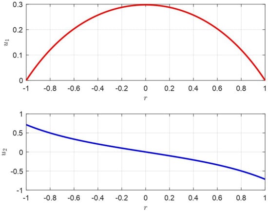 Figure 2. Recovering of the membrane by using the bvp4c MatLab® solver: , , .
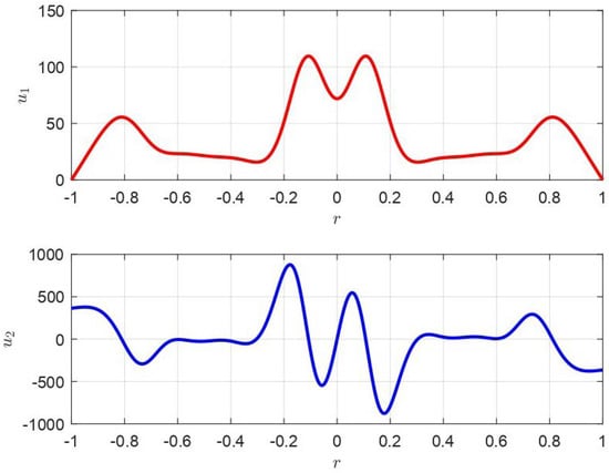 Figure 3. Recovering of the membrane by using the bvp4c MatLab® solver: , , .
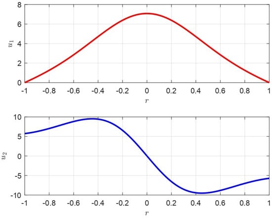 Figure 4. Recovering of the membrane by using the bvp4c MatLab® solver: , , and , .
 Figure 5. Recovering of the membrane by using the bvp4c MatLab® solver: , , and , .
 - , the numerical procedure does not work. It means that in (20) increases too much, (theoretically as ), so that the numerical procedure is forced to stop because the Jacobian matrix becomes singular.
- strong instabilities take place. In this case, even if the numerical procedure does not stop, instabilities next to the edge of the recovered membrane occurred. Figure 6 and Figure 7 display two examples of recovering of the membrane when highlighting strong instabilities of the membrane. In particular, Figure 6 has been achieved setting and , while Figure 7 has been obtained setting and . Obviously, depending on the considered initial data, the values of change for which one has no instabilities.
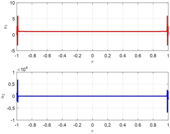 Figure 6. Recovering of the membrane achieved by and : strong instabilities take place next to the edge of the membrane.
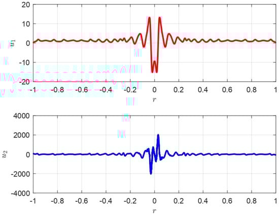 Figure 7. Recovering of the membrane achieved by and : strong instabilities take place next to the edge of the membrane.
Remark 12.
In the resolution of BVPs, an important aspect concerns the choice of initial conditions. The difficulty therefore lies in choosing suitable initial conditions that lead to a convergence of the method. Usually, if you know the progress of the solution, they are chosen in such a way as to be as accurate as possible, especially to achieve convergence and calculation time that is not too long. It starts by assigning values and proceeding with testing until the solution we expect is found. The results shown in Figure 3 highlight a non-convergence of the method; this is due to not "good" initial values. Furthermore, the different acceptable solution (Figure 2 and Figure 4) obtained with different initial values show how the BVPs cannot admit a single solution. (We only consider Figure 2 because the solution of the model must be lower than 1).
8.2. Order of Magnitude of According to the Analytical Condition of Uniqueness of the Solution
8.3. Characteristic Ranges of
Taking into account inequality (39), and remembering that, for , the numerical procedure converges in stability conditions, we can write:
from which:
Finally, from (41), it follows that . Then, the range of ensuring both convergence and stability is .
As shown above, , the numerical procedure does not work. In other words, the numerical procedure does not converge. In this case, it makes sense to write:
so that
Then, from (43), one can write , so that, , the numerical procedure does not converge.
If the numerical procedure converges with instability phenomena, . In this case, we can write:
for which it follows:
obtaining that, , the numerical procedure converges even if instability phenomena can occur next to the edges of the membrane.
9. Highlighting the Ghost Solutions’ Areas
To show the ghost solution areas, we start form the analytical inequality (39). Moreover, from equalty (3), we can write:
that, combining with equality (3), becomes:
Considering that the order of magnitude of , and are , and , respectively, from the inequality (47), we can write:
Then, it follows that the analytical condition (3) can be written as . Finally, , any solutions can be considered as ghost solutions. However, because , the numerical procedure does not converge; then, it follows that each numerical solution achieved is not a ghost solution. The results discussed in this Section are summarized in Table 1.

Table 1.
Convergence and stability areas.
10. Electromechanical Properties of the Membrane, Applied Voltage, and Ghost Solutions: Engineering Areas of Applicability of the Device
As discussed above, is very important for convergence of the numerical procedure and for its physical meaning as well. In particular, represents the proportionality between and [20]:
Moreover, depends on both V and the electromechanical properties of the material constituting the membrane. In fact, can be expressed as follows [20]:
where ( takes into account the electromechanical properties of the material constituting the membrane) and T is the mechanical tension of the membrane. Then, combining equality (49) with equality (50), we obtain:
Considering that, in dimensionless conditions, , and , from (53), the following inequality makes sense:
As known, can be expressed as (for details, see [19,20]):
from which, it follows that:
If the non convergence of the numerical procedure occurs, it makes sense to write the following chain of inequalities:
so that we can write:
Once the intended use of the device has been chosen (that is, once the pair has been fixed), from the inequality (59), is computable. In other words, once has been chosen, the material of the membrane is selected. Conversely, if the material of the membrane has been chosen (that is T has been fixed), it is possible to achieve the pair satisfying the inequality (60) (that is the intended use of the device).
11. Conclusions and Perspectives
In this paper, a numerical approach based on a three-stage Lobatto technique for recovering the profile of the membrane in an electrostatic circular MEMS is proposed. Mainly exploited as a numerical collocation technique for the resolution of BVPs, this procedure has been preferred to shooting methods because it usually requires the integration of IVPs being heavily unstable. The proposed numerical procedure has been applied to a well-known 2D nonlinear second-order differential model related to a circular membrane MEMS actuator in which the amplitude of the electrostatic field has been locally expressed in terms of the mean curvature of the membrane. The study of the convergence properties of the proposed method has allowed for highlighting the ranges of characteristic parameters (depending on both V and electromechanical properties of the material constituting the membrane) that ensure that the method can achieve convergence with or without instabilities. Furthermore, exploiting an algebraic inequality governing the existence of the solution for the differential model, the ranges of parameters (depending on the externally applied voltage) that ensure convergence (with or without instabilities) bringing out the ghost solutions’ areas have been evaluated. Finally, an algebraic inequality has been obtained, which allows for managing the choice of the intended use of the device once the electromechanical properties of the material constituting the membrane have been selected (and vice versa). The results we have obtained can be considered as encouraging. The tests have shown that the recovering of the membrane profile (in the absence of ghost solution, and a condition of convergence without instability) reach a maximum value at the center of the membrane of not less than 0.3, thus proving that the membrane offers an excellent response to the applied external voltage. Furthermore, the tests carried out have shown that the non-convergence area is extremely limited, thus guaranteeing a wide range of applicability of the device in industrial applications. However, we point out that the presence of instabilities makes the numerical approach not yet optimal, requiring further effort to reduce the instability zone as much as possible. This will be the subject of a future work.
Author Contributions
Conceptualization, M.V., G.A. and A.J.; methodology, M.V., G.A. and A.J.; investigation, M.V., G.A. and A.J. All authors have read and agreed to the published version of the manuscript.
Funding
This research received no external funding.
Conflicts of Interest
The authors declare no conflict of interest.
Abbreviations
The following abbreviations are used in this manuscript:
| R | radius of the device |
| V | applied voltage |
| electrostatic field | |
| magnitude of the electrostatic field | |
| r | radial coordinate |
| mean curvature | |
| profile of the membrane | |
| d | distance between the fixed plates |
| electrostatic pressure | |
| permittivity of the free space | |
| p | mechanical pressure |
| T | mechanical tension of the membrane |
| displacement of the membrane at | |
| k | constant of proportionalitycbetween and |
| electrostatic capacitance | |
| co-energy function | |
| q | electrostatic charge |
| electrostatic force | |
| bounded function depending on the dielectric properties | |
| function depending on V | |
| continuous function depending on r | |
| function depending both V and the electromechanical properties of the material constituting the membrane | |
| z | axe of symmetry |
| bi-Laplacian operator | |
| curvature | |
| function of proportionality | |
| critical security distance | |
| , | under and over solutions |
| U | |
| vector of unknown parameters | |
| boundary conditions | |
| cubic polynomial | |
| step-size | |
| residual | |
| MEMS | Micro-Electro-Mechanical Systems |
| BVP | Boundary Value Problem |
| ODE | Ordinary Differential Equation |
| IVP | Initial Value Problem |
| bvp4c | MatLab Subroutine to solve BVPs |
References
- Nathanson, N.H.; Newell, W.E.; Wickstrom, R.A.; Lewis, J.R. The Resonant Gate Transistor. IEEE Trans. Electron. Devices 1964, 14, 117–119. [Google Scholar] [CrossRef]
- Pelesko, J.A.; Bernstein, D.H. Modeling MEMS and NEMS; Chapman & Hall/CRC: Boca Raton, FL, USA; London, UK; New York, NY, USA; Washington, DC, USA, 2003. [Google Scholar]
- Di Barba, P.; Lorenzi, A. A Magneto-Thermo-Elastic Identification Problem with a Moving Boundary in a Micro-Device. Milan J. Math. 2013, 81, 347–383. [Google Scholar] [CrossRef]
- Jalali, E.; Akbari, O.A.; Sarafras, M.M.; Abbas, T.; Safaei, M.R. Heat Transfer of Oil/MWCNT Nanofluid Jet Injection Inside a Rectangular Microchannel. Simmetry 2019, 11, 757. [Google Scholar] [CrossRef]
- Sarafraz, M.M.; Hart, J.; Shrestha, E.; Arya, H.; Arjomandi, M. Experimental Thermal Energy Assessment of a Liquid Metal Eutectic in a Micrtochannel Heat Exchanger Equipped with a (10Hz/50Hz) Resonator. Appl. Therm. Eng. 2019, 148, 578–590. [Google Scholar] [CrossRef]
- Sarafraz, M.M.; Yang, B.; Ghomashchi, R. Fluid and Heat Trasnfer Characteristics of Aqueous Graphene Nanoplatelet (GNP) Nanofluid in a Microchannel. Physics 2019. [Google Scholar] [CrossRef]
- Selvakumar, V.S.; Sujatha, L.; Sundar, R. A Novel MEMS Microheater Based Alcohol Gas Sensor using Nanoparticle. J. Semicond. Technol. Sci. 2018, 18, 1–9. [Google Scholar] [CrossRef]
- Angiulli, G.; Versaci, M. Neuro-Fuzzy Network for the Design of Circular and Triangular Equilateral Microstrip Antennas. Int. J. Infrared Millim. Wavews 2002, 37, 1513–1520. [Google Scholar] [CrossRef]
- Farajpour, M.R.; Shahidi, A.R.; Farajpour, A. Influence of Initial Edge Displacement on the Nonlinear Vibration, Electrical and Magnetic Instabilities of Magneto-Electro-Elastic Nanofilms. Mech. Adv. Mater. Struct. 2019, 26, 1469–1481. [Google Scholar] [CrossRef]
- Mohammadi, A.K.; Ali, N.A. Effect of High Electrostatic Actuation on Thermoelastic Damping in Thin Rectangular Microplate Resonators. J. Theor. Appl. Mech. 2015, 53, 317–329. [Google Scholar] [CrossRef]
- Morabito, F.C.; Versaci, M. A Fuzzy Neural Approach to Localizing Holes in Conducting Plates. IEEE Trans. Magn. 2001, 37, 3534–3537. [Google Scholar] [CrossRef]
- Wang, F.; Zhang, L.; Li, L.; Wiao, Z.; Cao, Q. Design and Analysis of the Elastic-Beam Delaying Mechanism in a Micro-Mechanical Systems Device. Micromachines 2018, 9, 567. [Google Scholar] [CrossRef] [PubMed]
- Anjum, M.; Fida, A.; Ahmand, I.; Iftikhar, A. A Broadband Electromagnetic Type Energy Harvester for Smart Sensor Devices in Biomedical Applications. Sens. Actuators A Phys. 2018, 277, 52–59. [Google Scholar] [CrossRef]
- Ciuti, G.; Ricotti, L.; Menciassi, A.; Dario, P. MEMS Sensor Technologies for Human Centered Applications in Healthcare, Physical Activities, Safety and Environmental Sensing: A Review on Research Activities in Italy. Sensors 2015, 15, 6441–6468. [Google Scholar] [CrossRef] [PubMed]
- Kunti, G.; Dhar, J.; Bhattacharya, A.; Chakraborty, S. Electro-Thermally Driven Transport of a Non-Conducting Fluid in a Two-Layer System for MEMS and Biomedical Application. AIP J. Appl. Phys. 2018, 123, 1–18. [Google Scholar] [CrossRef]
- Di Barba, P.; Wiak, S. MEMS: Field Models and Optimal Design; Springer International Publishing: New York, NY, USA, 2020. [Google Scholar]
- Feng, J.; Liu, C.; Zhang, W.; Hao, S. Static and Dynamic Mechanical Behaviors of Electrostatic MEMS Resonator with Surface Processing Error. Micromachines 2018, 9, 34. [Google Scholar] [CrossRef] [PubMed]
- Maity, R.; Maity, N.P.; Baishya, S. Circular Membrane Approximation Model with the Effect of the Finiteness of the Electrode’s Diameter of MEMS Capacitive Micromachined Ultrasonic Transducers. Microsyst. Technol. 2017, 23, 3513–3524. [Google Scholar] [CrossRef]
- Di Barba, P.; Fattorusso, L.; Versaci, M. Electrostatic Field in Terms of Geometric Curvature in Membrane MEMS Devices. Commun. Appl. Ind. Math. 2017, 8, 165–184. [Google Scholar] [CrossRef]
- Angiulli, G.; Jannelli, A.; Morabito, F.C.; Versaci, M. Reconstructing the Membrane Detection of a 1D Electrostatic-Driven MEMS Device by the Shooting Method: Convergence Analysis and Ghost Solutions Identification. Comput. Appl. Math. 2018, 37, 4484–4498. [Google Scholar] [CrossRef]
- Versaci, M.; Angiulli, G.; Fattorusso, L.; Jannelli, A. On the Uniqueness of the Solution for a Semi-Linear Elliptic Boundary Value Problem of the Membrane MEMS Device for Reconstructing the Membrane Profile in Absence of Ghost Solutions. Int. J. Non-Linear Mech. 2019, 109, 24–31. [Google Scholar] [CrossRef]
- Di Barba, P.; Fattorusso, L.; Versaci, M. A 2D Non-Linear Second-Order Differential Model for Electrostatic Circular Membrane MEMS Devices: A Result of Existence and Uniqueness. Mathematics 2019, 9, 1193. [Google Scholar] [CrossRef]
- Versaci, M.; Morabito, F.C. Membrane Micro Electro-Mechanical Systems for Industrial Applications. In Handbook of Research on Advanced Mechatronic Systems and Intelligent Robotics; IGI Global: Pennsylvania, PA, USA, 2020. [Google Scholar]
- Ghosh, P. Numerical, Symbolic and Statistical Computing for Chemical Engineers Using MatLab®; Delhi 110092; PHI Learning: New Delhi, India, 2018. [Google Scholar]
- Timoshenko, S.; Woinowsky-Krieger, S. Theory of Plates and Shells; McGraw-Hill: New York, NY, USA, 1959. [Google Scholar]
- Cassani, D.; Fattorusso, L.; Tarsia, A. Non-local Dynamic Problems with Singular Nonlinearities and Application to MEMS. Prog. Nonlinear Differ. Equ. Appl. 2014, 85, 185–206. [Google Scholar]
- Russell, R.D.; Shampine, L.F. Numerical Methods for Singular Boundary Value Problems. SIAM J. Numer. Anal. 1975, 12, 13–36. [Google Scholar] [CrossRef]
- Fazio, R.; Jannelli, A. BVPs on infinite intervals: A test problem, a non-standard finite difference scheme and a posteriori error estimator. Math. Methods Appl. Sci. 2017, 40, 6285–6294. [Google Scholar] [CrossRef]
© 2020 by the authors. Licensee MDPI, Basel, Switzerland. This article is an open access article distributed under the terms and conditions of the Creative Commons Attribution (CC BY) license (http://creativecommons.org/licenses/by/4.0/).