Dimensionality-reduction Procedure for the Capacitated p-Median Transportation Inventory Problem

Abstract

The capacitated p-median transportation inventory problem with heterogeneous fleet (CLITraP-HTF) aims to determine an optimal solution to a transportation problem subject to location-allocation, inventory management and transportation decisions. The novelty of CLITraP-HTF is to design a supply chain that solves all these decisions at the same time. Optimizing the CLITraP-HTF is a challenge because of the high dimension of the decision variables that lead to a large and complex search space. The contribution of this paper is to develop a dimensionality-reduction procedure (DRP) to reduce the CLITraP-HTF complexity and help to solve it. The proposed DRP is a mathematical proof to demonstrate that the inventory management and transportation decisions can be solved before the optimization procedure, thus reducing the complexity of the CLITraP-HTF by greatly narrowing its number of decision variables such that the remaining problem to solve is the well-known capacitated p-median problem (CPMP). The conclusion is that the proposed DRP helps to solve the CLITraP-HTF because the CPMP can be and has been solved by applying different algorithms and heuristic methods.

1. Introduction

The capacitated p-median transportation inventory problem with heterogeneous fleet model (CLITraP-HTF) is a non-linear-mixed-integer problem (MINLP). The CLITraP-HTF is used to design the supply chain network (SCN) of any product that aims to determine an optimal solution to a transportation problem subject to extra constraints that locate supply and customers facilities, to manage the inventory of all facilities in a SCN, and to manage a fleet of vehicles characterized by different capacities and costs for the distribution of a product. The model constraints consider: distribution centres, facilities storage capacity, facilities safety stock, specific facilities operational inventory requirements, vehicles with different load capacities, un-divisible load, for each customer demand is stochastic and behaves as a normal distribution function, operational inventory requirements, lead time is not variable, and a continuous review inventory policy is applied.

The CLITraP-HTF solves the capacitated p-median problem (CPMP) decision variables (location-allocation) plus inventory management, fleet assignment, transportation, and level of service decision variables. The CPMP is a p-median problem (PMP) restricted to the capacity of the vehicles that are used to transport certain product. The PMP is a non-deterministic polynomial-time hardness (NP-hard) problem [1]. Since the CLITraP-HTF solves the PMP decision variables, it is possible to classify the CLITraP-HTF as a NP-hard problem too. NP-hard problem means, any algorithm would be very hard computing time consuming to attain the optimal solution in polynomial time [2]. The PMP has been optimally solved in polynomial time for small instances by Hakimi [3] and Daskin and Maass [4], other researchers have applied different optimization algorithms such as branch and bound algorithms [5,6,7] and special decomposition algorithms [8,9]. It is more difficult to solve the CLITraP-HTF than the PMP because the CLITraP-HTF solves more decision variables than the PMP, meaning that the dimension of the CLITraP-HTF is larger and more complex than the PMP.

The number of decision variables to be solved is very important when solving an optimization model, because computational difficulties are due to a substantial degree by the number of them [10]. The optimization problem suffers from a dimensionality problem because as the number of decision variables to solve increases, the complications of finding a global optimal solution increases too [11]. It is because the search space for finding a global optimal solution grows as the dimensions of the decision variables increases [12,13]. One option to solve a high dimensionality optimization problem, such as the CLITraP-HTF, in polynomial time is to sacrifice optimality by finding a feasible solution with a heuristic method, but an optimal solution is probably not achieved. Another option is to relax the complexity of the problem by reducing the number of decision variables to solve with a dimensionality-reduction procedure (DRP) [11]. Sometimes, it is possible to optimally solve NP-hard problems whether the number of decision variables is sufficiently reduced, but whether it is not, a heuristic method needs to be developed, in any case, at least the complexity of the problem is reduced.

This paper aims to develop a DRP which yields to solve the CLITraP-HTF. The DRP developed in this paper is a mathematical proof (Section 3) that helps to solve the CLITraP-HTF, the distribution between facilities is always made with a single type of vehicle, the one with the cheapest cost, and by sending only one shipment every replenishment period. When solving these transportation decisions, the replenishment period decisions (one for each connection between facilities), the number of shipments between facilities per order or per replenishment period using the chosen vehicle type, the investment decisions, and the level of service decision variables are also solved, all before the application of an optimization methodology. The DRP solves these decision variables and the remining problem to solve is the CPMP. It is because, the remaining decision variables to be solved with an optimization methodology are the location and the allocation once. As it is mentioned above, since the CPMP can be solved with different optimization methodologies such as branch and bound, and special decomposition, then the CLITraP-HTF can be solved too.

Section 2 outlines the CLITraP-HTF. Section 3 develops the mathematical proof or proposed DRP. In Section 4, the proposed DRP is applied to different scenarios. Finally, Section 5 discuss and concludes this paper.

2. The Capacitated p-Median Transportation Inventory Problem with Heterogeneous Fleet

Carmona-Benitez et al. [14] published a location-allocation inventory-routing problem (LIRP) with heterogeneous fleet of vehicles. However, their model has three limitations: first, their model assumes that the lead times (L) are the same for all customer facilities no matter who is the supplier facility, but in a real life problem, lead times are different depending the distance between origin facilities and destination facilities; second, their model assumes that the variability of the demand over lead time (σ_DL) does not change when a facility is chosen to be a DC, however, in a real-life problem, the σ_DL changes when a facility is assigned to be a DC; third, in their model product enters the network through only one supplier facility, but in a real-life problem, product could enter through different facilities. In this paper, the LIRP proposed in Carmona-Benitez et al. [14] is modified to overcome these limitations in Section 2.3, and it is called CLITraP-HTF.

The LIRP presented by Carmona-Benitez et al. [14] is based on a real company distribution problem, where vehicles are not allowed to supply more than one facility per trip because the hazardous material (hazmat) product they distribute is not divisible by law. It is a very uncommon restriction in supply chain, because vehicles usually can supply product to different customers in a route. Hence, the LIRP published in Carmona-Benitez et al. [14] is not a routing problem because it does not solve routing decisions, it is a transportation problem, because it solves transportation decisions, reason why, in this paper, the CLITraP-HTF is classified as a transportation problem.

2.1. Strategic Decisions Assumptions

The CLITraP-HTF solves tactical decisions [15]. The CLITraP-HTF designs SCNs for companies with certain characteristics. First, the costs of the location of DCs and the allocation of facilities to DCs must be cheap. Second, facilities can become DCs or cease to be DCs depending on their demand changes over time. These characteristics make location-allocation decisions tactical and not strategic, as they normally are [15,16]. Third, all facilities can be operated as DC, also tactical decisions. Fourth, the model designs SCNs for products with highly stochastic and dynamic demand with changes in short periods of time. Fifth, vehicles are prohibited to supply more than one facility per trip.

2.2. Definition and Notations

The CLITraP-HTF works with three set of facilities (Table 1).

Table 1. CLITraP-HTF set of facilities.

Set	Definition
O {1, …, l}	is the set of all external suppliers’ facilities that supply product to the system or supply chain
V {l + 1, …, i}	is the set of all facilities that can be DC or not, and
V {l + 1, …, j}	is also the set of customer facilities
W {1, …, w}	is the set of types of vehicles

The CLITraP-HTF have Boolean, Integer, and Continuous decision variables (Table 2).

Table 2. CLITraP-HTF decision variables.

Variable	Definition	Type	Units
Xi	is equal to 1 if facility i ϵ V is operated as DC, 0 otherwise	Boolean	-
Xl	is equal to 1 for all external supplier facilities l ϵ O	Boolean	-
Yij	is equal to 1 if the link connecting facility i ϵ {O ∪ V} with facility j ϵ V is used to transport product from facility i ϵ {O ∪ V} to facility j ϵ V	Boolean	-
δj	is equal to 1 if facility i ϵ V requires an investment	Boolean	-
TH	is the time horizon (i.e., annual, semi-annual, monthly)	Integer	year
p	determines the maximum number of DCs that can be located	Integer	-
nijw	is the number of shipments per order or per replenishment period using vehicle w ϵ W to transport product from facility i ϵ {O ∪ V} to facility j ϵ V	Integer	shipments/order
Tj	is the replenishment period in which facility j ϵ V must be supplied	Continuous	days/order
qijw	is the replenishment amount of product shipped from facility i ϵ V to facility j ϵ V using vehicle type w ϵ W	Continuous	unit/shipment
αij	is the inventory service level at facility j ϵ V when it is supplied by facility i ϵ {O ∪ V}	Continuous	-

Table 3 and Table 4 show the the CLITraP-HTF parameters.

Table 3. CLITraP-HTF parameters [17].

Parameter	Definition	Units
Qij	is the total replenishment amount of product shipped per order from facility i ϵ {O ∪ V} to facility j ϵ V	unit/order
Cijw	is the costs of shipping product from facility i ϵ V to facility j ϵ V using vehicle type w ϵ W	$/shipment
c	is the purchase cost	$/unit
cti	is the ordering cost also known as setup cost	$/order
cei	is the carrying or holding cost at facility i ϵ V; Equal to (c ir)	$/unit/year
Cui	is the penalty cost per shortage or unfulfilled demand unit at facility i ϵ V	$/unit
yij	is the shortage or unfulfilled demand at facility j ϵ V when its supplier is facility i ϵ {O ∪ V}	units
TIi	is the total inventory for facility i ϵ V during time Ti	units day/order
λi	is the average daily demand at facility i ϵ V	units/day
Λi	is the sum of average daily demand of facility i ϵ V and the demands of the facilities j ϵ V supplied by facility i ϵ V	units/day
IOpi	is the minimum number of days in inventory required to operate facility i ϵ V	units
ROPij	is the reorder point at facility j ϵ V when its supplier is facility i ϵ {O ∪ V}	units
ssij	is the safety stock at facility j ϵ V when its supplier is facility i ϵ {O ∪ V}	units
Lij	is the order lead time at facility j ϵ V when its supplier is facility i ϵ {O ∪ V}	days
σLij	is the Lij standard deviation at facility j ϵ V when its supplier is facility i ϵ {O ∪ V}	days
sDLij	is the standard deviation of demand over the Lij at facility j ϵ V when its supplier is facility i ϵ {O ∪ V}	units
σDLi	is the standard deviation of demand over the lead calculated from the sum of the variances at facility i ϵ V and the variances of the facilities j ϵ V supplied by facility i ϵ V	units
$\overline{{\mathrm{x}}_{\mathrm{ij}}}$	is the mean of lead time demand of facility j ϵ {O ∪ V} when its supplier is facility i ϵ {O ∪ V}	units
σij	is the standard deviation of lead time demand of facility j ϵ {O ∪ V} when its supplier is facility i ϵ {O ∪ V}	units
ir	is the capital cost rate (Timme and Williams-Timme, 2003)	1/year
Capi	is the total storage capacity at facility i ϵ V	units
CapNi	is the current storage capacity at facility i ϵ V	units
CapIi	is an extra storage capacity at facility i ϵ V that can be available only if an investment is made	units

Table 4. CLITraP-HTF parameters.

Parameter	Definition	Units
VCapw	is the carrying capacity of vehicle type w ϵ W	units
Kl	is the quantity of product offered at external supplier facility l ϵ O	units
P	is the product price per unit	$/unit
Invui	is the investment unit cost required at facility i ϵ V to increased storage capacity CapIi	$/unit
FCi	is the location costs of a DC at facility i ϵ V	$
TrCijw	is the total shipping cost from facility i ϵ {O ∪ V} to facility j ϵ V with vehicle type w ϵ W in TH	$
Pcij	is the stock-out or shortage cost at facility j ϵ V because of facility i ϵ V	$
ICi	is the total inventory cost for facility i ϵ V in TH	$
OpCi	is the opportunity cost for facility i ϵ V in TH	$
INVi	is the investment cost for facility i ϵ V in TH	$
FLCi	is the facility location cost of a DC on facility i ϵ V (payable only once per TH)	$
TC	is the total cost in TH	$

Objective Function

The model objective function (TC) considers the costs of transportation (Equation (1)), the costs of investment (Equation (2)), the costs of facility location (Equation (3)), the costs of opportunity (Equation (4)), and the costs of inventory (Equation (5)) which includes the costs of purchasing, the costs of holding the inventory (Equation (6)), the costs of ordering or setup costs, and the costs of shortage (Equation (7)).

$${\mathrm{TrC}}_{\mathrm{i}\mathrm{j}\mathrm{w}}={\mathrm{C}}_{\mathrm{i}\mathrm{j}\mathrm{w}}{\mathrm{n}}_{\mathrm{i}\mathrm{j}\mathrm{w}}{\mathrm{Y}}_{\mathrm{i}\mathrm{j}}\left(\mathrm{T}\mathrm{H}/{\mathrm{T}}_{\mathrm{j}}\right),$$

(1)

$$\mathrm{I}\mathrm{N}{\mathrm{V}}_{\mathrm{j}}={\mathsf{\delta }}_{\mathrm{j}}\mathrm{C}\mathrm{a}\mathrm{p}{\mathrm{I}}_{\mathrm{j}}\mathrm{I}\mathrm{n}\mathrm{v}{\mathrm{u}}_{\mathrm{j}}\hspace{1em}\forall \mathrm{j}\in \mathrm{V},$$

(2)

$$\mathrm{F}\mathrm{L}{\mathrm{C}}_{\mathrm{j}}=\mathrm{F}{\mathrm{C}}_{\mathrm{j}}{\mathrm{X}}_{\mathrm{j}}\hspace{1em}\forall \mathrm{j}\in \mathrm{V},$$

(3)

$$\mathrm{O}\mathrm{p}{\mathrm{C}}_{\mathrm{i}\mathrm{j}}=\mathrm{T}{\mathrm{I}}_{\mathrm{i}\mathrm{j}}\mathrm{P}\mathrm{i}\mathrm{r}{\mathrm{Y}}_{\mathrm{i}\mathrm{j}}\left(\mathrm{T}\mathrm{H}/{\mathrm{T}}_{\mathrm{j}}\right),$$

(4)

$$\mathrm{I}{\mathrm{C}}_{\mathrm{i}\mathrm{j}}=\left\{\mathrm{c}{\Lambda }_{\mathrm{j}}{\mathrm{T}}_{\mathrm{j}}+\mathrm{c}{\mathrm{e}}_{\mathrm{j}}\mathrm{T}{\mathrm{I}}_{\mathrm{i}\mathrm{j}}+\mathrm{c}{\mathrm{t}}_{\mathrm{j}}+\mathrm{P}{\mathrm{c}}_{\mathrm{i}\mathrm{j}}\right\}{\mathrm{Y}}_{\mathrm{i}\mathrm{j}}\left(\mathrm{T}\mathrm{H}/{\mathrm{T}}_{\mathrm{j}}\right),$$

(5)

where:

$$\mathrm{T}{\mathrm{I}}_{\mathrm{i}\mathrm{j}}=\left(\mathrm{s}{\mathrm{s}}_{\mathrm{i}\mathrm{j}}+\mathrm{I}\mathrm{O}{\mathrm{p}}_{\mathrm{j}}\right){\mathrm{T}}_{\mathrm{j}}+{\Lambda }_{\mathrm{j}}{\mathrm{T}}_{\mathrm{j}}^2/2=\left[{\mathrm{L}}_{\mathrm{j}}{\Lambda }_{\mathrm{j}}+{\mathsf{\sigma }}_{\mathrm{D}\mathrm{L}\mathrm{j}}\mathrm{F}{\left({\mathrm{a}}_{\mathrm{j}}\right)}^{-1}+\mathrm{I}\mathrm{O}{\mathrm{p}}_{\mathrm{j}}\right]{\mathrm{T}}_{\mathrm{j}}+{\Lambda }_{\mathrm{j}}{\mathrm{T}}_{\mathrm{j}}^2/2\hspace{1em}\forall \mathrm{j}\in \mathrm{V},$$

(6)

$$\mathrm{P}{\mathrm{c}}_{\mathrm{i}\mathrm{j}}=\mathrm{E}\left(\mathrm{C}{\mathrm{u}}_{\mathrm{j}}{\mathrm{y}}_{\mathrm{i}\mathrm{j}}\right)=\mathrm{C}{\mathrm{u}}_{\mathrm{j}}\left[\left(1-{\mathsf{\alpha }}_{\mathrm{i}\mathrm{j}}\right)\left({\stackrel{\_}{{\displaystyle \mathrm{x}}}}_{\mathrm{i}\mathrm{j}}-{\mathrm{F}}^{-1}\left({\mathsf{\alpha }}_{\mathrm{i}\mathrm{j}}\right)\right)+\left({\mathsf{\sigma }}_{\mathrm{i}\mathrm{j}}/\sqrt{2\mathsf{\pi }}\right)\left[{\mathrm{e}}^{-0.5\left(\left({\mathrm{F}}^{-1}\left({\mathsf{\alpha }}_{\mathrm{i}\mathrm{j}}\right)-{\stackrel{\_}{{\displaystyle \mathrm{x}}}}_{\mathrm{i}\mathrm{j}}\right)/{\mathsf{\sigma }}_{\mathrm{i}\mathrm{j}}\right)}\right]\right],$$

(7)

where:

$${\stackrel{\_}{{\displaystyle \mathrm{x}}}}_{\mathrm{i}\mathrm{j}}={\Lambda }_{\mathrm{j}}{\mathrm{L}}_{\mathrm{i}\mathrm{j}},$$

(8)

$${\mathsf{\sigma }}_{\mathrm{i}\mathrm{j}}^2={\mathrm{L}}_{\mathrm{i}\mathrm{j}}{\mathsf{\sigma }}_{\mathrm{D}\mathrm{L}\mathrm{j}}^2+{\Lambda }_{\mathrm{j}}^2{\mathsf{\sigma }}_{\mathrm{L}\mathrm{i}\mathrm{j}}^2,$$

(9)

In Appendix A, Pc_ij is derived explicitly.

2.3. Mixed Integer Programming Model (MIP)

$$\mathrm{M}\mathrm{I}\mathrm{N}\left\{{\displaystyle \sum _{\mathrm{i}=1}^{\mathrm{v}}{\displaystyle \sum _{\begin{array}{l}\mathrm{j}=\mathrm{o}+1\\ \mathrm{i}\ne \mathrm{j}\end{array}}^{\mathrm{v}}{\displaystyle \sum _{\mathrm{w}=1}^{\mathrm{w}}\left[\mathrm{T}\mathrm{r}{\mathrm{C}}_{\mathrm{i}\mathrm{j}\mathrm{w}}\right]}+{\displaystyle \sum _{\mathrm{i}=1}^{\mathrm{v}}{\displaystyle \sum _{\mathrm{j}=\mathrm{o}+1}^{\mathrm{v}}\left[\mathrm{I}{\mathrm{C}}_{\mathrm{i}\mathrm{j}}+\mathrm{O}\mathrm{p}{\mathrm{C}}_{\mathrm{i}\mathrm{j}}\right]}}+{\displaystyle \sum _{\mathrm{j}=\mathrm{o}+1}^{\mathrm{v}}\left[\mathrm{I}\mathrm{N}{\mathrm{V}}_{\mathrm{j}}+\mathrm{F}\mathrm{L}{\mathrm{C}}_{\mathrm{j}}\right]}}}\right\},$$

(10)

$${\displaystyle \sum _{\mathrm{i}=\mathrm{o}+1}^{\mathrm{v}}{\mathrm{X}}_{\mathrm{i}}\le \mathrm{p}}1\le \mathrm{p}\le \mathrm{v}-\mathrm{l},$$

(11)

$${\displaystyle \sum _{\mathrm{i}=1}^{\mathrm{v}}{\mathrm{Y}}_{\mathrm{i}\mathrm{j}}=1}\hspace{1em}\forall \mathrm{j}\in \mathrm{V},\mathrm{i}\ne \mathrm{j},$$

(12)

$${\mathrm{Y}}_{\mathrm{i}\mathrm{j}}-{\mathrm{X}}_{\mathrm{i}}\le 0\hspace{1em}\forall \mathrm{i}\in \left\{\mathrm{O}\cup \mathrm{V}\right\},\forall \mathrm{j}\in \mathrm{V},\mathrm{i}\ne \mathrm{j},$$

(13)

$${\Lambda }_{\mathrm{i}}={\mathsf{\lambda }}_{\mathrm{i}}+{\displaystyle \sum _{\mathrm{j}=\mathrm{o}+1}^{\mathrm{v}}{\mathsf{\lambda }}_{\mathrm{j}}{\mathrm{Y}}_{\mathrm{i}\mathrm{j}}}\forall \mathrm{i}\in \left\{\mathrm{O}\cup \mathrm{V}\right\},\mathrm{i}\ne \mathrm{j},$$

(14)

$${\mathsf{\sigma }}_{\mathrm{D}\mathrm{L}\mathrm{i}}^2={\mathrm{s}}_{\mathrm{D}\mathrm{L}\mathrm{i}}^2+{\displaystyle \sum _{\mathrm{j}=\mathrm{o}+1}^{\mathrm{v}}{\mathrm{s}}_{\mathrm{D}\mathrm{L}\mathrm{j}}^2{\mathrm{Y}}_{\mathrm{i}\mathrm{j}}}\forall \mathrm{i}\in \left\{\mathrm{O}\cup \mathrm{V}\right\},\mathrm{i}\ne \mathrm{j},$$

(15)

$${\displaystyle \sum _{\mathrm{i}=1}^{\mathrm{v}}\left[\left({\displaystyle \sum _{\mathrm{w}=1}^{\mathrm{w}}{\mathrm{q}}_{\mathrm{i}\mathrm{j}\mathrm{w}}{\mathrm{n}}_{\mathrm{i}\mathrm{j}\mathrm{w}}}\right){\mathrm{Y}}_{\mathrm{i}\mathrm{j}}\right]-\left[\left(\mathrm{C}\mathrm{a}\mathrm{p}{\mathrm{N}}_{\mathrm{j}}+\mathrm{C}\mathrm{a}\mathrm{p}{\mathrm{I}}_{\mathrm{j}}{\mathsf{\delta }}_{\mathrm{j}}-\mathrm{I}\mathrm{O}{\mathrm{p}}_{\mathrm{j}}\right)\right]\le 0}\forall \mathrm{j}\in \mathrm{V},\mathrm{i}\ne \mathrm{j},$$

(16)

$${\displaystyle \sum _{\mathrm{i}=1}^{\mathrm{v}}}\left[\left({\displaystyle \sum _{\mathrm{w}=1}^{\mathrm{w}}{\mathrm{q}}_{\mathrm{i}\mathrm{j}\mathrm{w}}{\mathrm{n}}_{\mathrm{i}\mathrm{j}\mathrm{w}}}\right){\mathrm{Y}}_{\mathrm{i}\mathrm{j}}\right]-({\Lambda }_{\mathrm{j}}{\mathrm{T}}_{\mathrm{j}})\ge 0\hspace{1em}\forall \mathrm{j}\in \mathrm{V},\mathrm{i}\ne \mathrm{j},$$

(17)

$${\mathrm{K}}_{\mathrm{l}}-{\Lambda }_{\mathrm{l}}\ge 0\forall \mathrm{l}\in \left\{\mathrm{O}\right\},$$

(18)

$${\mathrm{q}}_{\mathrm{i}\mathrm{j}\mathrm{w}}-\mathrm{V}\mathrm{C}\mathrm{a}{\mathrm{p}}_{\mathrm{w}}\le 0\forall \mathrm{i}\in \{\mathrm{O}\cup \mathrm{V}\},\forall \mathrm{j}\in \mathrm{V},\forall \mathrm{w}\in \mathrm{W},$$

(19)

$${\mathrm{n}}_{\mathrm{i}\mathrm{j}\mathrm{w}}\in {\mathrm{Z}}^{+},$$

(20)

$${\mathrm{X}}_{\mathrm{i}}\in \{0,1\}\forall \mathrm{i}\in \mathrm{V},$$

(21)

$${\mathrm{Y}}_{\mathrm{i}\mathrm{j}}\in \{0,1\}\forall \mathrm{i}\in \left\{\mathrm{O}\cup \mathrm{V}\right\},\forall \mathrm{j}\in \mathrm{V},\mathrm{i}\ne \mathrm{j},$$

(22)

$${\mathsf{\delta }}_{\mathrm{i}}\in \{0,1\}\forall \mathrm{i}\in \mathrm{V},$$

(23)

$${\mathrm{T}}_{\mathrm{i}}>0\forall \mathrm{i}\in \mathrm{V},$$

(24)

$$0<{\mathsf{\alpha }}_{\mathrm{i}\mathrm{j}}<1\forall \mathrm{i}\in \mathrm{V},$$

(25)

The model minimizes the total cost for the TH (Equation (10)); the cost is calculated by the sum of Equation (1) to Equation (5), Equation (10) first term is for facility i ϵ {O ∪ V}, facility j ϵ V and i ≠ j, and vehicle type w ϵ W, Equation (10) s term is for facility i ϵ {O ∪ V} and for facility j ϵ V, and Equation (10) third term is for facility j ϵ V. Equation (11) indicates that the maximum number of DCs that can be located is limited to p. Possible connections are between facilities i ϵ {O ∪ V} and facilities j ϵ V. Each facility j ϵ V can be supplied by one DC located in facility i ϵ V or by one external facility i ϵ O (Equation (12)) but not for more than one facility i ϵ {O ∪ V}. Facility j ϵ V can be supplied from facility i ϵ V only if facility i ϵ V is selected as DC (Equation (13)). Equations (11)–(13) are the location-allocation restrictions. Λ_i calculates the total demand of facility i ϵ {O ∪ V}, as the sum of its demand (λ_i) plus the sum of the demands of the facilities j’s ϵ V it is assigned to supply (λ_j) (Equation (14)). σ²_DLi calculates the lead time variance of facility i ϵ {O ∪ V}, which is equal to the sum of its variance (s²_DLi) plus the sum of the variance of the facilities j´s ϵ V it is assigned to supply (s²_DLj) (Equation (15)). The amount of product supplied to facility j ϵ V during T_j, is equal to the multiplication of q_ijw by n_ijw. The Cap_j of facility j ϵ V is compose by CapN_j plus CapI_j, the left-over capacity is equal to Cap_j minus IOp_j. The total quantity of product to supply from all the facilities i´s ϵ {O ∪ V}, with a certain number of shipments n_ijw, using different types of vehicles w´s ϵ W, to facility j ϵ V must be lower than facility j ϵ V remaining capacity (Equation (16)). The total amount of product supplied from all the facilities i´s ϵ {O ∪ V}, with a certain number of shipments n_ijw, using different types of vehicles w´s ϵ W, to facility j ϵ V in time T_j, must be higher than or equal to the demand of facility j ϵ V in time T_j (Equation (17)). The total K offered by external facility l ϵ O must be higher than or equal to the total amount of product demanded from all the facilities j´s ϵ V it supplies, daily (Equation (18)). The amount of product to be shipped from facility i ϵ {O ∪ V} to facility j ϵ V with a vehicle type w ϵ W must be less than or equal to the capacity of vehicle type w ϵ W (Equation (19)). n_ijw is an integer variable that must be higher than or equal to zero (Equation (20)). Equation (16) to Equation (20) are for the inventory management and product transportation, vehicles visit no more than one facility j ϵ V per trip, and they use different types of vehicles w´s ϵ W. Equation (21)–(23) are binary constraints. Equation (24) are nonnegativity constraints different from zero, and Equation (25) indicate that the level of services of each facility i ϵ V is between 0 and 1.

3. Dimensionality-Reduction Procedure

Section 3.1 mathematically proofs that in the CLITraP-HTF the inventory-transport decision variables (n, T and q) and the investment decision variables (δ) can be solved before applying the optimization methodology. Section 3.2 mathematically proofs that in the CLITraP-HTF the inventory level decision variables (α) can be solved prior to starting the optimization methodology. Section 3.1 and Section 3.2 propose a DRP that reduces the CLITraP-HTF degree of computational difficulties and helps to solve this high complex problem.

3.1. Dimensionality-Reduction Procedure on the Inventory-Transport and Investment Decisions Variables

In the CLITraP-HTF the objective function is convex in T_j > 0. From Equation (10), it is possible to compute the optimal value of T_j by taking the derivate of the objective function with respect to T_j (Equation (10)).

$${\mathrm{T}}_{\mathrm{j}}^{*}=\sqrt{\frac{{\displaystyle \sum _{\mathrm{w}=1}^{\mathrm{w}}{\mathrm{C}}_{\mathrm{i}\mathrm{j}\mathrm{w}}{\mathrm{n}}_{\mathrm{i}\mathrm{j}\mathrm{w}}}+\mathrm{c}{\mathrm{t}}_{\mathrm{j}}+\mathrm{P}{\mathrm{c}}_{\mathrm{i}\mathrm{j}}}{{\Lambda }_{\mathrm{j}}\left(\mathrm{P}\mathrm{i}\mathrm{r}+\mathrm{c}{\mathrm{e}}_{\mathrm{j}}\right)}},$$

(26)

In Equation (26), the optimal value of T^*_j depends on finding the optimal values of the variables n_ijw and Y_ijw.

For the demonstration on the dimensionality reduction of inventory-transport and investment decision variables, let start analyzing the total cost of transporting product from facility i ϵ {O ∪ V} to facility j ϵ V using a vehicle type w ϵ W when w = 1 (homogeneous fleet). From Equation (10), the total cost every T_j is calculated as follows:

$$\mathrm{T}\mathrm{C}{\mathrm{p}}_{\mathrm{i}\mathrm{j}}={\mathrm{C}}_{\mathrm{i}\mathrm{j}}{\mathrm{n}}_{\mathrm{i}\mathrm{j}}+\left\{\mathrm{c}{\Lambda }_{\mathrm{j}}{\mathrm{T}}_{\mathrm{j}}+\left(\mathrm{c}{\mathrm{e}}_{\mathrm{j}}+\mathrm{P}\mathrm{i}\mathrm{r}\right)\left(\mathrm{T}{\mathrm{I}}_{\mathrm{i}\mathrm{j}}\right)+\mathrm{c}{\mathrm{t}}_{\mathrm{j}}+\mathrm{P}{\mathrm{c}}_{\mathrm{i}\mathrm{j}}\right\}+\left\{\mathrm{C}\mathrm{a}\mathrm{p}{\mathrm{I}}_{\mathrm{j}}\mathrm{I}\mathrm{n}\mathrm{v}{\mathrm{u}}_{\mathrm{j}}{\mathsf{\delta }}_{\mathrm{j}}+\mathrm{F}{\mathrm{C}}_{\mathrm{j}}{\mathrm{X}}_{\mathrm{j}}\right\}{\mathrm{T}}_{\mathrm{j}}/\mathrm{T}\mathrm{H},$$

(27)

The optimum value of n_ij is an integer variable different from zero because the amount of product to transport from facility i ϵ {O ∪ V} to facility j ϵ V every T^*_j is equal to Λ_jT^*_j and to n_ijq_ij (Equation (28)). Λ_jT^*_j is different from zero because Equations (24) and (14) indicate that T^*_j and Λ_j are positive and different from zero respectively.

$${\Lambda }_{\mathrm{j}}{\mathrm{T}}_{\mathrm{j}}^{*}={\mathrm{n}}_{\mathrm{i}\mathrm{j}}{\mathrm{q}}_{\mathrm{i}\mathrm{j}},$$

(28)

From Equations (27) and (28), it is possible to conclude that the minimum TCp_ij is when n_ij = 1. Therefore, only one shipment using a vehicle of type w must be used to transport product from facility i ϵ {O ∪ V} to facility j ϵ V every T^*_j. Even if the Λ_j increases or decreases, n_ij is equal to 1, it does not matter if facility j ϵ V is chosen to be a DC or not.

By substituting Equation (28) into Equation (26) when n_ij = 1 and when w = 1 (homogeneous fleet), T^*_j is equal to:

$${\mathrm{T}}_{\mathrm{j}}^{*}=\frac{{\mathrm{C}}_{\mathrm{i}\mathrm{j}}{\mathrm{n}}_{\mathrm{i}\mathrm{j}}+\mathrm{c}{\mathrm{t}}_{\mathrm{j}}+\mathrm{P}{\mathrm{c}}_{\mathrm{i}\mathrm{j}}}{{\mathrm{q}}_{\mathrm{i}\mathrm{j}}\left(\mathrm{P}\mathrm{i}\mathrm{r}+\mathrm{c}{\mathrm{e}}_{\mathrm{j}}\right)},$$

(29)

Equation (30) calculates TCp_ij in terms of q_ij when n_ij = 1 by substituting Equation (29) into Equation (27):

$$\begin{array}{l}\mathrm{T}\mathrm{C}{\mathrm{p}}_{\mathrm{i}\mathrm{j}}={\mathrm{C}}_{\mathrm{i}\mathrm{j}}{\mathrm{n}}_{\mathrm{i}\mathrm{j}}+\mathrm{c}{\mathrm{t}}_{\mathrm{j}}+\mathrm{P}{\mathrm{c}}_{\mathrm{i}\mathrm{j}}+\left[\mathrm{c}{\Lambda }_{\mathrm{j}}+\frac{\mathrm{C}\mathrm{a}\mathrm{p}{\mathrm{I}}_{\mathrm{j}}\mathrm{I}\mathrm{n}\mathrm{v}{\mathrm{u}}_{\mathrm{j}}{\mathsf{\delta }}_{\mathrm{j}}+\mathrm{F}{\mathrm{C}}_{\mathrm{j}}{\mathrm{X}}_{\mathrm{j}}}{\mathrm{T}\mathrm{H}}\right]\left(\frac{{\mathrm{C}}_{\mathrm{i}\mathrm{j}}{\mathrm{n}}_{\mathrm{i}\mathrm{j}}+\mathrm{c}{\mathrm{t}}_{\mathrm{j}}+\mathrm{P}{\mathrm{c}}_{\mathrm{i}\mathrm{j}}}{{\mathrm{q}}_{\mathrm{i}\mathrm{j}}\left(\mathrm{P}\mathrm{i}\mathrm{r}+\mathrm{c}{\mathrm{e}}_{\mathrm{j}}\right)}\right)+\\ \left(\mathrm{c}{\mathrm{e}}_{\mathrm{j}}+\mathrm{P}\mathrm{i}\mathrm{r}\right)\left[\left(\mathrm{s}{\mathrm{s}}_{\mathrm{i}\mathrm{j}}+\mathrm{I}\mathrm{o}{\mathrm{p}}_{\mathrm{j}}\right)\left(\frac{{\mathrm{C}}_{\mathrm{i}\mathrm{j}}{\mathrm{n}}_{\mathrm{i}\mathrm{j}}+\mathrm{c}{\mathrm{t}}_{\mathrm{j}}+\mathrm{P}{\mathrm{c}}_{\mathrm{i}\mathrm{j}}}{{\mathrm{q}}_{\mathrm{i}\mathrm{j}}\left(\mathrm{P}\mathrm{i}\mathrm{r}+\mathrm{c}{\mathrm{e}}_{\mathrm{j}}\right)}\right)+\frac{{\Lambda }_{\mathrm{j}}}{2}{\left(\frac{{\mathrm{C}}_{\mathrm{i}\mathrm{j}}{\mathrm{n}}_{\mathrm{i}\mathrm{j}}+\mathrm{c}{\mathrm{t}}_{\mathrm{j}}+\mathrm{P}{\mathrm{c}}_{\mathrm{i}\mathrm{j}}}{{\mathrm{q}}_{\mathrm{i}\mathrm{j}}\left(\mathrm{P}\mathrm{i}\mathrm{r}+\mathrm{c}{\mathrm{e}}_{\mathrm{j}}\right)}\right)}^2\right]\end{array}$$

(30)

From Equation (30), the larger the value of q_ij the lower the TCp_ij what is consistent with the theory of economies of scale. The value of q_ij must be as large as possible to minimize TCp_ij, and it is restricted by VCap_w and the storage capacity at facility j ϵ V (Cap_j). Since, Cap_j can increase from CapN_j to CapN_j + CapI_j whether an investment is done, the value of q_ij also depends on the decision investment variable δ_j. The decision variables q_ij and δ_j are solved as follows:

• Whether $\mathrm{V}\mathrm{C}\mathrm{a}{\mathrm{p}}_{\mathrm{w}}\le \mathrm{C}\mathrm{a}\mathrm{p}{\mathrm{N}}_{\mathrm{j}}\mathrm{then}{\mathrm{q}}_{\mathrm{i}\mathrm{j}}=\mathrm{V}\mathrm{C}\mathrm{a}{\mathrm{p}}_{\mathrm{w}}\mathrm{and}{\mathsf{\delta }}_{\mathrm{j}}=0$; otherwise,
• Whether
  $\mathrm{V}\mathrm{C}\mathrm{a}{\mathrm{p}}_{\mathrm{w}}\ge \mathrm{C}\mathrm{a}\mathrm{p}{\mathrm{N}}_{\mathrm{j}}\mathrm{a}\mathrm{n}\mathrm{d}\mathrm{V}\mathrm{C}\mathrm{a}{\mathrm{p}}_{\mathrm{w}}\le \left(\mathrm{C}\mathrm{a}\mathrm{p}{\mathrm{N}}_{\mathrm{j}}+\mathrm{C}\mathrm{a}\mathrm{p}{\mathrm{I}}_{\mathrm{j}}\right)\mathrm{and}{\mathrm{C}}_{\mathrm{i}\mathrm{j}}\frac{{\Lambda }_{\mathrm{j}}}{\mathrm{C}\mathrm{a}\mathrm{p}{\mathrm{N}}_{\mathrm{j}}}\le \left[{\mathrm{C}}_{\mathrm{i}\mathrm{j}}\frac{{\Lambda }_{\mathrm{j}}}{\mathrm{V}\mathrm{C}\mathrm{a}{\mathrm{p}}_{\mathrm{w}}}+\frac{\mathrm{C}\mathrm{a}\mathrm{p}{\mathrm{I}}_{\mathrm{j}}\mathrm{I}\mathrm{n}\mathrm{v}{\mathrm{u}}_{\mathrm{j}}}{\mathrm{T}\mathrm{H}}\right]$$\mathrm{then}{\mathrm{q}}_{\mathrm{i}\mathrm{j}}=\mathrm{C}\mathrm{a}\mathrm{p}{\mathrm{N}}_{\mathrm{j}}\mathrm{and}{\mathsf{\delta }}_{\mathrm{j}}=0$; Otherwise,
• Whether
  $\mathrm{V}\mathrm{C}\mathrm{a}{\mathrm{p}}_{\mathrm{w}}\ge \mathrm{C}\mathrm{a}\mathrm{p}{\mathrm{N}}_{\mathrm{j}}\mathrm{a}\mathrm{n}\mathrm{d}\mathrm{V}\mathrm{C}\mathrm{a}{\mathrm{p}}_{\mathrm{w}}\le \left(\mathrm{C}\mathrm{a}\mathrm{p}{\mathrm{N}}_{\mathrm{j}}+\mathrm{C}\mathrm{a}\mathrm{p}{\mathrm{I}}_{\mathrm{j}}\right)\mathrm{and}{\mathrm{C}}_{\mathrm{i}\mathrm{j}}\frac{{\Lambda }_{\mathrm{j}}}{\mathrm{C}\mathrm{a}\mathrm{p}{\mathrm{N}}_{\mathrm{j}}}\ge \left[{\mathrm{C}}_{\mathrm{i}\mathrm{j}}\frac{{\Lambda }_{\mathrm{j}}}{\mathrm{V}\mathrm{C}\mathrm{a}{\mathrm{p}}_{\mathrm{w}}}+\frac{\mathrm{C}\mathrm{a}\mathrm{p}{\mathrm{I}}_{\mathrm{j}}\mathrm{I}\mathrm{n}\mathrm{v}{\mathrm{u}}_{\mathrm{j}}}{\mathrm{T}\mathrm{H}}\right]$$\mathrm{then}{\mathrm{q}}_{\mathrm{i}\mathrm{j}}=\mathrm{V}\mathrm{C}\mathrm{a}{\mathrm{p}}_{\mathrm{w}}\mathrm{and}{\mathsf{\delta }}_{\mathrm{j}}=1$; Otherwise,
• Whether
  $\mathrm{V}\mathrm{C}\mathrm{a}{\mathrm{p}}_{\mathrm{w}}\ge \left(\mathrm{C}\mathrm{a}\mathrm{p}{\mathrm{N}}_{\mathrm{j}}+\mathrm{C}\mathrm{a}\mathrm{p}{\mathrm{I}}_{\mathrm{j}}\right)\mathrm{then}{\mathrm{q}}_{\mathrm{i}\mathrm{j}}=\left(\mathrm{C}\mathrm{a}\mathrm{p}{\mathrm{N}}_{\mathrm{j}}+\mathrm{C}\mathrm{a}\mathrm{p}{\mathrm{I}}_{\mathrm{j}}\right)\mathrm{and}{\mathsf{\delta }}_{\mathrm{j}}=1$

Finally, knowing the value of n_ij and q_ij, Equation (29) calculates the value of T^*_j.

So far, for a homogeneous fleet of vehicles type w, it is being proved that in the CLITraP-HTF, the inventory-transport decision variables (n, T and q) and the investment decision variables (δ) can be solved before the optimization.

Now, the dimensionality reduction of inventory-transport and investment decisions for a heterogeneous capacity fleet of vehicles is demonstrated as follows: Let us analyze the total cost of transporting product from facility i ϵ {O ∪ V} to facility j ϵ V using vehicles with different load capacities (w ϵ W). From Equation (10), the total cost every T_j is calculated as follows:

$$\mathrm{T}\mathrm{C}{\mathrm{p}}_{\mathrm{i}\mathrm{j}}={\displaystyle \sum _{\mathrm{w}=1}^{\mathrm{W}}{\mathrm{C}}_{\mathrm{i}\mathrm{j}\mathrm{w}}{\mathrm{n}}_{\mathrm{i}\mathrm{j}\mathrm{w}}}+\left\{\mathrm{c}{\Lambda }_{\mathrm{j}}{\mathrm{T}}_{\mathrm{j}}+\left(\mathrm{c}{\mathrm{e}}_{\mathrm{j}}+\mathrm{P}\mathrm{i}\mathrm{r}\right)\mathrm{T}{\mathrm{I}}_{\mathrm{i}\mathrm{j}}+\mathrm{c}{\mathrm{t}}_{\mathrm{j}}+\mathrm{P}{\mathrm{c}}_{\mathrm{i}\mathrm{j}}\right\}+\left\{\mathrm{C}\mathrm{a}\mathrm{p}{\mathrm{I}}_{\mathrm{j}}\mathrm{I}\mathrm{n}\mathrm{v}{\mathrm{u}}_{\mathrm{j}}{\mathsf{\delta }}_{\mathrm{j}}+\mathrm{F}{\mathrm{C}}_{\mathrm{j}}{\mathrm{X}}_{\mathrm{j}}\right\}{\mathrm{T}}_{\mathrm{j}}/\mathrm{T}\mathrm{H},$$

(31)

From Equation (31), the optimum transportation cost ${\displaystyle \sum _{\mathrm{w}=1}^{\mathrm{W}}{\mathrm{C}}_{\mathrm{i}\mathrm{j}\mathrm{w}}{\mathrm{n}}_{\mathrm{i}\mathrm{j}\mathrm{w}}}$ is achieved when ${\displaystyle \sum _{\mathrm{w}=1}^{\mathrm{W}}{\mathrm{n}}_{\mathrm{i}\mathrm{j}\mathrm{w}}}=1$, because the amount of product to transport from facility i ϵ {O ∪ V} to facility j ϵ V every T^*_j using vehicle w ϵ W is equal to Λ_jT^*_j and to n_ijwq_ijw. Λ_jT^*_j is different from zero because Equations (24) and (14) indicate that T^*_j and Λ_j are positive and different from zero respectively. Hence, only one shipment using one type of vehicle from the heterogeneous fleet of vehicles w ϵ W is used to transport product from facility i ϵ {O ∪ V} to facility j ϵ V every T_j, even if Λ_j in facility j ϵ V increases or decreases, or whether facility j ϵ V is chosen to be a DC or not.

Equation (32) chooses the vehicle w ϵ W that must be used to transport product from facility i ϵ {O ∪ V} to facility j ϵ V every T^*_j. Equation (34) chooses the vehicle based on the minimum TCp_ij (Equation (29)) calculated for each vehicle w ϵ W when n_ij = 1.

$$\mathrm{T}\mathrm{C}{\mathrm{p}}_{\mathrm{i}\mathrm{j}}=\min \left(\mathrm{T}\mathrm{C}{\mathrm{p}}_{\mathrm{i}\mathrm{j}}\left(\mathrm{w}=1\right),\mathrm{T}\mathrm{C}{\mathrm{p}}_{\mathrm{i}\mathrm{j}}\left(\mathrm{w}=2\right),\dots ,\mathrm{T}\mathrm{C}{\mathrm{p}}_{\mathrm{i}\mathrm{j}}\left(\mathrm{w}=\mathrm{W}\right)\right),$$

(32)

The solution to the CLITraP-HTF, presented in Section 3.2, is to distribute product from facility i ϵ {O ∪ V} to facility j ϵ V every T_j using the vehicle that achieves the lowest TCp_ij (Equation (32)) from the heterogeneous fleet of vehicles w ϵ W.

3.2. Dimensionality-Reduction Procedure on the Level of Service Decision Variables

This section mathematically demonstrates that α_ij can be solved prior to starting the solution method, reducing the degree of computational difficulties.

In the CLITraP-HTF, demand is stochastic. There are different ways to operate an inventory system with random demand. The CLITraP-HTF considers the (ROP, Q) inventory policy. In this policy, the inventory level is observed always. When the level drops to ROP, an order Q is placed. The order Q arrives to replenish the inventory after L which is assumed known and constant. In this policy, the values of ROP and Q are the two decisions required. The values of ROP depend on the values of α because ROP is calculated as the inverse cumulative normal distribution of the level of service (F⁻¹(α)). Figure 1 demonstrates that F(ROP_ij) = α_ij or ROP_ij = F⁻¹(α_ij), and it is computed as:

$$\mathrm{p}\left({\mathrm{x}}_{\mathrm{i}\mathrm{j}}>\mathrm{R}\mathrm{O}{\mathrm{P}}_{\mathrm{i}\mathrm{j}}\right)=1-\mathrm{p}\left({\mathrm{x}}_{\mathrm{i}\mathrm{j}}\le \mathrm{R}\mathrm{O}{\mathrm{P}}_{\mathrm{i}\mathrm{j}}\right)=1-\mathrm{F}\left({\mathrm{x}}_{\mathrm{i}\mathrm{j}}\le \mathrm{R}\mathrm{O}{\mathrm{P}}_{\mathrm{i}\mathrm{j}}\right)=1-{\mathsf{\alpha }}_{\mathrm{i}\mathrm{j}},$$

(33)

where: x_ij is the lead time demand also known as order placed or order fulfillment.

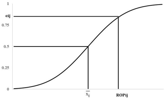
Figure 1. Cumulative normal demand distribution.

The (ROP, Q) inventory policy is most concerned with the possibility of stock-out or shortage. If y_ij is the shortage or unfulfilled demand at facility j ϵ V when its supplier is facility i ϵ {O ∪ V}, then:

$${\mathrm{y}}_{\mathrm{i}\mathrm{j}}={\mathrm{x}}_{\mathrm{i}\mathrm{j}}-\mathrm{R}\mathrm{O}{\mathrm{P}}_{\mathrm{i}\mathrm{j}},$$

(34)

The variability of the demand during L must be considered to calculate the probability of shortage:

$$\mathrm{p}\left({\mathrm{y}}_{\mathrm{i}\mathrm{j}}>0\right)=\mathrm{p}\left({\mathrm{x}}_{\mathrm{i}\mathrm{j}}-\mathrm{R}\mathrm{O}{\mathrm{P}}_{\mathrm{i}\mathrm{j}}>0\right)=\mathrm{p}\left({\mathrm{x}}_{\mathrm{i}\mathrm{j}}>\mathrm{R}\mathrm{O}{\mathrm{P}}_{\mathrm{i}\mathrm{j}}\right)=1-{\mathsf{\alpha }}_{\mathrm{i}\mathrm{j}},$$

(35)

Subsequently, Pc can be calculated as:

$$\mathrm{P}{\mathrm{c}}_{\mathrm{i}\mathrm{j}}=\mathrm{E}\left(\mathrm{C}{\mathrm{u}}_{\mathrm{i}}{\mathrm{y}}_{\mathrm{i}\mathrm{j}}\right)=\mathrm{C}{\mathrm{u}}_{\mathrm{i}}\mathrm{E}\left({\mathrm{y}}_{\mathrm{i}\mathrm{j}}\right)=\mathrm{C}{\mathrm{u}}_{\mathrm{i}}\mathrm{E}\left({\mathrm{x}}_{\mathrm{i}\mathrm{j}}-\mathrm{R}\mathrm{O}{\mathrm{P}}_{\mathrm{i}\mathrm{j}}\right)=\mathrm{C}{\mathrm{u}}_{\mathrm{i}}{\displaystyle \underset{\mathrm{R}\mathrm{O}{\mathrm{P}}_{\mathrm{i}\mathrm{j}}}{\overset{\infty }{\int }}\left({\mathrm{x}}_{\mathrm{i}\mathrm{j}}-\mathrm{R}\mathrm{O}{\mathrm{P}}_{\mathrm{i}\mathrm{j}}\right)\mathrm{f}\left({\mathrm{x}}_{\mathrm{i}\mathrm{j}}\right)\mathrm{d}{\mathrm{x}}_{\mathrm{i}\mathrm{j}}},$$

(36)

Equation (36) shows that Pc depends on the values of α because ROP depends on the values of α. Appendix A demonstrates that PC_ij is computed in terms of α_ij during T_j, as it is expressed in Equation (7).

In this section, for the demonstration on the dimensionality reduction of α, let analyse the total cost (Equation (7)) of transporting product from facility i ϵ {O ∪ V} to facility j ϵ V using a fleet of vehicles type w ϵ W. This paper follows the mathematical demonstration developed by Carmona-Benitez et al. [14] to calculate the optimum values of the α decision variables. As it is mentioned in Section 2, the difference between their demonstration and our demonstration is that the CLITraP-HTF recognizes that lead times are different depending on the distance between a facility i ϵ {O ∪ V} and a facility j ϵ V, the variability of the demands change for those facilities that are chosen to be DCs, and product can enter through more than one facility to the network.

The α decision variables represent the expected probability of not incurring in a stock-out during lead time. α_ij means the trade-off between the different costs, TrC_ijw (Equation (1)), INV_i (Equation (2)), FLC_i (Equation (3)), OpC_ij (Equation (4)), IC_ij (Equation (5)) and Pc_ij (Equation (7)), among a facility i ϵ {O ∪ V} and facility j ϵ V. Therefore, the proposed optimization approach requires the existence of an equilibrium condition between TrC_ijw, INV_i, FLC_i, OpC_ij, IC_ij and Pc_ij (Equation (37)) for the distribution of a product between a facility i ϵ {O ∪ V} and a facility j ϵ V,

$$\frac{\partial \mathrm{G}\left({\mathsf{\alpha }}_{\mathrm{i}\mathrm{j}}\right)}{\partial {\mathsf{\alpha }}_{\mathrm{i}\mathrm{j}}}=-{\displaystyle \sum _{\mathrm{i}=0}^{\mathrm{V}}\frac{\partial \mathrm{P}{\mathrm{c}}_{\mathrm{i}\mathrm{j}}}{\partial {\mathsf{\alpha }}_{\mathrm{i}\mathrm{j}}}},$$

(37)

where

$$\frac{\partial \mathrm{G}\left({\mathsf{\alpha }}_{\mathrm{i}\mathrm{j}}\right)}{\partial {\mathsf{\alpha }}_{\mathrm{i}\mathrm{j}}}={\displaystyle \sum _{\mathrm{w}=0}^{\mathrm{W}}{\displaystyle \sum _{\mathrm{i}=0}^{\mathrm{V}}\frac{\partial \mathrm{I}{\mathrm{C}}_{\mathrm{i}\mathrm{j}}}{\partial {\mathsf{\alpha }}_{\mathrm{i}\mathrm{j}}}}}+{\displaystyle \sum _{\mathrm{i}=0}^{\mathrm{V}}\frac{\partial \mathrm{O}\mathrm{p}{\mathrm{C}}_{\mathrm{i}\mathrm{j}}}{\partial {\mathsf{\alpha }}_{\mathrm{i}\mathrm{j}}}+}{\displaystyle \sum _{\mathrm{i}=0}^{\mathrm{V}}\frac{\partial \mathrm{F}\mathrm{L}{\mathrm{C}}_{\mathrm{i}}}{\partial {\mathsf{\alpha }}_{\mathrm{i}\mathrm{j}}}}+{\displaystyle \sum _{\mathrm{i}=0}^{\mathrm{V}}\frac{\partial \mathrm{I}\mathrm{N}{\mathrm{V}}_{\mathrm{i}}}{\partial {\mathsf{\alpha }}_{\mathrm{i}\mathrm{j}}}}+{\displaystyle \sum _{\mathrm{i}=0}^{\mathrm{V}}{\displaystyle \sum _{\mathrm{j}=0}^{\mathrm{V}}{\displaystyle \sum _{\mathrm{w}=0}^{\mathrm{W}}\frac{\partial \mathrm{T}\mathrm{r}{\mathrm{C}}_{\mathrm{i}\mathrm{j}\mathrm{w}}}{\partial {\mathsf{\alpha }}_{\mathrm{i}\mathrm{j}}}}}}.$$

(38)

For the distribution of a product between a facility i ϵ {O ∪ V} and a facility j ϵ V, Equation (37) requires derivatives of IC_ij, OpC_ij, FLC_i, INV_i, TrC_ijw and Pc_ij in terms of T_i, X_i, Y_ij, q_ijw, n_ijw, δ_i and α_ij. These derivatives are very tough. However, Section 3.1 mathematically demonstrates that T_i, q_ijw, n_ijw, and δ_i can be solved prior to starting the optimization methodology, and for the case of the distribution of a product between facility i ϵ {O ∪ V} and facility j ϵ V, the decision variables X_i and Y_ij does not exist. So, the complexity of them is avoided.

Carmona-Benitez et al. [14] develop an approach to optimize α_ij before the solution method is applied. Their approach optimizes the costs in terms of T_i and α_ij simultaneously. This is possible because these variables are mutually dependent, and because an optimum value of α_ij exists for every value of T_i. Knowing the optimum value of T_i, it is possible to find the equilibrium condition in terms of α_ij for each T_i. In this paper, their approach is explained in detail to demonstrate the optimal solution of α_ij because it is part of the DRP proposed in this paper.

Equation (39) computes the equilibrium condition, where the related CLITraP-HTF decision variables are fixed (T_i, q_ijw, n_ijw, and δ_i).

$$\begin{array}{l}\frac{\partial \mathrm{G}\left({\mathsf{\alpha }}_{\mathrm{i}\mathrm{j}}/{\mathrm{X}}_{\mathrm{i}}\left({\mathsf{\alpha }}_{\mathrm{i}\mathrm{j}}\right),{\mathrm{Y}}_{\mathrm{i}\mathrm{j}}\left({\mathsf{\alpha }}_{\mathrm{i}\mathrm{j}}\right),{\mathrm{T}}_{\mathrm{i}}\left({\mathsf{\alpha }}_{\mathrm{i}\mathrm{j}}\right),{\mathsf{\delta }}_{\mathrm{i}}\left({\mathsf{\alpha }}_{\mathrm{i}\mathrm{j}}\right),{\mathrm{q}}_{\mathrm{i}\mathrm{j}\mathrm{w}}\left({\mathsf{\alpha }}_{\mathrm{i}\mathrm{j}}\right),{\mathrm{n}}_{\mathrm{i}\mathrm{j}\mathrm{w}}\left({\mathsf{\alpha }}_{\mathrm{i}\mathrm{j}}\right)\right)}{\partial {\mathsf{\alpha }}_{\mathrm{i}\mathrm{j}}}=\\ -{\displaystyle \sum _{\mathrm{i}=0}^{\mathrm{V}}\frac{\partial \mathrm{P}{\mathrm{c}}_{\mathrm{i}\mathrm{j}}\left({\mathsf{\alpha }}_{\mathrm{i}\mathrm{j}}/{\mathrm{X}}_{\mathrm{i}}\left({\mathsf{\alpha }}_{\mathrm{i}\mathrm{j}}\right),{\mathrm{Y}}_{\mathrm{i}\mathrm{j}}\left({\mathsf{\alpha }}_{\mathrm{i}\mathrm{j}}\right),{\mathrm{T}}_{\mathrm{i}}\left({\mathsf{\alpha }}_{\mathrm{i}\mathrm{j}}\right),{\mathsf{\delta }}_{\mathrm{i}}\left({\mathsf{\alpha }}_{\mathrm{i}\mathrm{j}}\right),{\mathrm{q}}_{\mathrm{i}\mathrm{j}\mathrm{w}}\left({\mathsf{\alpha }}_{\mathrm{i}\mathrm{j}}\right),{\mathrm{n}}_{\mathrm{i}\mathrm{j}\mathrm{w}}\left({\mathsf{\alpha }}_{\mathrm{i}\mathrm{j}}\right)\right)}{\partial {\mathsf{\alpha }}_{\mathrm{i}\mathrm{j}}}}\end{array}$$

(39)

Equation (39) is equal to Equation (37) for different values of α_ij, and inside a specific neighborhood of these values. Equation (40) explains that this equality is caused by the evenness of the network configuration in the declared neighborhood:

$$\frac{\partial \mathrm{G}\left({\mathsf{\alpha }}_{\mathrm{i}\mathrm{j}}\right)}{\partial {\mathsf{\alpha }}_{\mathrm{i}\mathrm{j}}}=-{\displaystyle \sum _{\mathrm{i}=0}^{\mathrm{V}}\left[\frac{\partial \mathrm{P}{\mathrm{c}}_{\mathrm{i}\mathrm{j}}}{\partial {\mathsf{\alpha }}_{\mathrm{i}\mathrm{j}}}\right]},$$

(40)

The marginal shortage costs (Equation (40)) are calculated to find the optimal value of αij:

$$\begin{array}{l}-{\displaystyle \sum _{\mathrm{i}=0}^{\mathrm{V}}\frac{\partial \mathrm{P}{\mathrm{c}}_{\mathrm{i}\mathrm{j}}\left({\mathsf{\alpha }}_{\mathrm{i}\mathrm{j}}/{\mathrm{X}}_{\mathrm{i}}\left({\mathsf{\alpha }}_{\mathrm{i}\mathrm{j}}\right),{\mathrm{Y}}_{\mathrm{i}\mathrm{j}}\left({\mathsf{\alpha }}_{\mathrm{i}\mathrm{j}}\right),{\mathrm{T}}_{\mathrm{i}}\left({\mathsf{\alpha }}_{\mathrm{i}\mathrm{j}}\right),{\mathsf{\delta }}_{\mathrm{i}}\left({\mathsf{\alpha }}_{\mathrm{i}\mathrm{j}}\right),{\mathrm{q}}_{\mathrm{i}\mathrm{j}\mathrm{w}}\left({\mathsf{\alpha }}_{\mathrm{i}\mathrm{j}}\right),{\mathrm{n}}_{\mathrm{i}\mathrm{j}\mathrm{w}}\left({\mathsf{\alpha }}_{\mathrm{i}\mathrm{j}}\right)\right)}{\partial {\mathsf{\alpha }}_{\mathrm{i}\mathrm{j}}}}=\\ -\mathrm{C}{\mathrm{u}}_{\mathrm{i}\mathrm{j}}\left[-\left(1-{\mathsf{\alpha }}_{\mathrm{i}\mathrm{j}}\right)\frac{\partial \mathrm{R}\mathrm{O}{\mathrm{P}}_{\mathrm{i}\mathrm{j}}}{\partial {\mathsf{\alpha }}_{\mathrm{i}\mathrm{j}}}\right]\end{array}$$

(41)

The operating marginal costs are expressed as follows:

$$\frac{\partial \mathrm{G}\left({\mathsf{\alpha }}_{\mathrm{i}\mathrm{j}}/{\mathrm{X}}_{\mathrm{i}}\left({\mathsf{\alpha }}_{\mathrm{i}\mathrm{j}}\right),{\mathrm{Y}}_{\mathrm{i}\mathrm{j}}\left({\mathsf{\alpha }}_{\mathrm{i}\mathrm{j}}\right),{\mathrm{T}}_{\mathrm{i}}\left({\mathsf{\alpha }}_{\mathrm{i}\mathrm{j}}\right),{\mathsf{\delta }}_{\mathrm{i}}\left({\mathsf{\alpha }}_{\mathrm{i}\mathrm{j}}\right),{\mathrm{q}}_{\mathrm{i}\mathrm{j}\mathrm{w}}\left({\mathsf{\alpha }}_{\mathrm{i}\mathrm{j}}\right),{\mathrm{n}}_{\mathrm{i}\mathrm{j}\mathrm{w}}\left({\mathsf{\alpha }}_{\mathrm{i}\mathrm{j}}\right)\right)}{\partial {\mathsf{\alpha }}_{\mathrm{i}\mathrm{j}}}=-\left({\mathrm{h}}_{\mathrm{j}}+\mathrm{P}\mathrm{i}\mathrm{r}\right){\mathrm{T}}_{\mathrm{j}}\frac{\partial \mathrm{R}\mathrm{O}{\mathrm{P}}_{\mathrm{i}\mathrm{j}}}{\partial {\mathsf{\alpha }}_{\mathrm{i}\mathrm{j}}},$$

(42)

By substituting Equations (41) and (42) in Equation (40), the equilibrium and optimization condition is calculated:

$$\left({\mathrm{h}}_{\mathrm{j}}+\mathrm{P}\mathrm{i}\mathrm{r}\right){\mathrm{T}}_{\mathrm{j}}\frac{\partial \mathrm{R}\mathrm{O}{\mathrm{P}}_{\mathrm{i}\mathrm{j}}}{\partial {\mathsf{\alpha }}_{\mathrm{i}\mathrm{j}}}=\mathrm{C}{\mathrm{u}}_{\mathrm{i}\mathrm{j}}\left[-\left(1-{\mathsf{\alpha }}_{\mathrm{i}\mathrm{j}}\right)\frac{\partial \mathrm{R}\mathrm{O}{\mathrm{P}}_{\mathrm{i}\mathrm{j}}}{\partial {\mathsf{\alpha }}_{\mathrm{i}\mathrm{j}}}\right],$$

(43)

Finally, Equation (44) calculates the optimal value of α_ij in terms of T_j:

$${\mathsf{\alpha }}_{\mathrm{i}\mathrm{j}}=1-\frac{\left({\mathrm{h}}_{\mathrm{j}}+\mathrm{P}\mathrm{i}\mathrm{r}\right){\mathrm{T}}_{\mathrm{j}}}{\mathrm{C}{\mathrm{u}}_{\mathrm{i}\mathrm{j}}},$$

(44)

Hence, the optimal value of α_ij can be calculated when T_j is known.

Finally, since Kariv and Hakimi [1] prove that the PMP is a NP-hard problem, and this paper proves the CPMP is a subproblem of the CLITraP-HTF, then it is possible to conclude that the CLITraP-HTF is a NP-hard problem too.

4. Results

Equation (45) calculates the total number of variables to be solved in the CLITraP-HTF. The dimensionality of decision variables growths as the number of facilities rises. Therefore, the total number of variables cause a considerable degree of computational difficulties in solving the CLITraP-HTF.

Equation (45) calculates the complexity of the CLITraP-HTF in terms of number of variables to solve. The complexity of the CLITraP-HTF increases mainly because the decision variables Y, q and n exponentially increase as the number of facilities (v) and types of vehicles (w) increase.

$$\mathrm{Total}\mathrm{number}\mathrm{of}\mathrm{variables}=\left[1+\mathrm{v}\left(4+\left(2\mathrm{w}+1\right)\left(\mathrm{v}-1\right)\right)\right],$$

(45)

As an example, Table 5 shows the CLITraP-HTF dimension of decision variables for scenarios with different number of facilities and for three different types of vehicles (w = 3). Table 5 indicates that the number of variables to solve increases as the number of facilities growths, following an exponential distribution (Figure 2). Equation (45) results clearly show that the CLITraP-HTF is an optimization problem that suffers from a dimensionality problem, because as the number of facilities to consider increases, the number of decision variables also increase (Table 5). It is major problem because the SCN of a real company connects many facilities making difficult to use the CLITraP-HTF to design a real company SCN.

Table 5. CLITraP-HTF dimension of decision variables for scenarios with different number of facilities.

Decision Variables	Number of Facilities (Small Size Instances)
	2	22	42	62	82	102	122	142	162	182
X	2	22	42	62	82	102	122	142	162	182
Δ	2	22	42	62	82	102	122	142	162	182
T	2	22	42	62	82	102	122	142	162	182
A	2	22	42	62	82	102	122	142	162	182
Y	2	462	1722	3782	6642	10,302	14,762	20,022	26,082	32,942
q	6	1386	5166	11,346	19,926	30,906	44,286	60,066	78,246	98,826
n	6	1386	5166	11,346	19,926	30,906	44,286	60,066	78,246	98,826
p	1	1	1	1	1	1	1	1	1	1
Total	23	3323	12,223	26,723	46,823	72,523	103,823	140,723	183,223	231,323

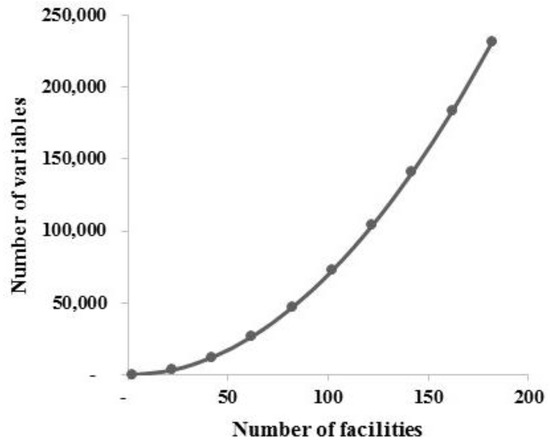
Figure 2. CLITraP-HTF total number of decision variables.

Table 5 shows that in the CLITraP-HTF most of the decision variables are of the type Y, n, and q. For a large size instances with 1,500,000 facilities, using Equation (45), the total number of variables are equal to 15.75 × 10¹² or 15.75 trillion; for a medium size instance with 20,000 facilities, the total number of variables is equal to 400 million. Equation (45) shows how high are the dimensionality of decision variables of large and medium size CLITraP-HTF.

Equation (46) calculates the complexity of the CLITraP-HTF in terms of number of scenarios that must be solved to find a global optimal solution. The scenarios originate from the combination of the decision variables X, Y, δ, and p. In Equation (46), the decision variables n, T, q, and α are not considered because they are either integer or continuous. The complexity of the CLITraP-HTF increases as the number of facilities (v), the number of types of vehicles (w), and the number of DC to be located increase.

$$\mathrm{E}=\left[\left(\mathrm{v}+{\displaystyle \sum _{\mathrm{p}=2}^{\mathrm{v}-1}\left\{{\displaystyle \sum _{\mathrm{i}=1}^{\mathrm{v}-2}\left\{\left(\begin{array}{l}\mathrm{V}\\ \mathrm{p}\end{array}\right)\mathrm{p}\left(\mathrm{i}+1\right)\right\}}\right\}}\right)\mathrm{w}+1\right]2^{\mathrm{v}},$$

(46)

Table 6 shows the number of scenarios or solutions that must be evaluated in the CLITraP-HTF for a different number of facilities and for three different types of vehicles (w = 3). Equation (46) has been code in Matlab 13b to calculate the number of scenarios (Table 6). Matlab is not capable to calculate the number of scenarios for the case of medium and large size instances, in fact, it can calculate not more than v = 170 facilities with 8.20 E + 108 scenarios. Equation (46) results clearly show that the CLITraP-HTF is a huge combinatorial problem because as the number of facilities to consider in a SCN increases, the search space (number of scenarios to be evaluated) for finding a global optimal solution increases too. Equation (46) results also show that reaching a global optimal solution to the CLITraP-HTF is very hard.

Table 6. CLITraP-HTF search space for scenarios with different number of facilities.

	Number of Facilities (Small Size Instances)
	2	22	42	62	82	102	122	142	162
Scenarios	28	1.33 × 1017	1.05 × 1030	3.74 × 1042	9.55 × 1054	2.03 × 1067	3.82 × 1079	6.63 × 1091	1.08 × 10104

Dimensionality-Reduction Proceedure Results

This section shows that the DRP highly reduces the complexity of the CLITraP-HTF. Section 3.1 demonstrates that in the CLITraP-HTF, the inventory-transport decision variables (n, T and q) and the investment decision variables (δ) can be solved before the optimization solution by applying the proposed DRP to minimize the complexity of the CLITraP-HTF. Equation (47) calculates the complexity of the remaining problem in terms of number of variables to solve. The complexity of the remaining problem increases because the decision variables Y increase as the number of facilities (v) increases.

$$\mathrm{Total}\mathrm{number}\mathrm{of}\mathrm{variables}=\left[1+\mathrm{v}\left(\mathrm{v}-1\right)+2\mathrm{v}\right],$$

(47)

Table 7 shows the dimension of the decision variables after applying the proposed DRP on the inventory-transport decision variables (n, T and q) and the investment decision variables (δ) for the same example shown in Table 5.

Table 7. CLITraP-HTF dimension of decision variables after applying the DRP on n, T, q and δ.

Decision Variables	Number of Facilities (Small Size Instances)
	2	22	42	62	82	102	122	142	162	182
X	2	22	42	62	82	102	122	142	162	182
α	2	22	42	62	82	102	122	142	162	182
Y	2	462	1722	3782	6642	10,302	14,762	20,022	26,082	32,942
p	1	1	1	1	1	1	1	1	1	1
Total	7	507	1807	3907	6807	10,507	15,007	20,307	26,407	33,307

In Figure 3, the black line shows the number of variables to be evaluated by the CLITraP-HTF before applying the proposed DRP to solve variables n, T, q and δ; and the grey line shows the remaining variables to be evaluated.

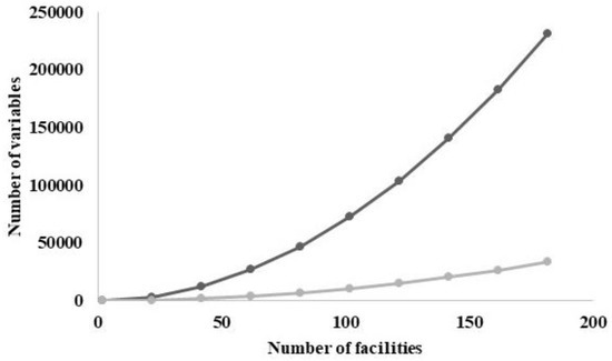
Figure 3. CLITraP-HTF number of decision variables after applying the DRP on n, T, q and δ.

Section 3.2 demonstrates that in the CLITraP-HTF, the level of services decision variables (α’s) can be solved before the optimization solution. Equation (48) calculates the number of variables after the proposed DRP is applied (Section 3.1 and Section 3.2).

$$\mathrm{Total}\mathrm{number}\mathrm{of}\mathrm{variables}=\left[{\mathrm{v}}^2+1\right],$$

(48)

Table 8 shows the dimension of the decision variables after applying the proposed DRP (Section 3.1 and Section 3.2) on the level of service decision variables (α) for the same example shown in Table 5 and Table 6 as comparison to the number of variables.

Table 8. CLITraP-HTF dimension of decision variables after applying a DRP on α.

Decision Variables	Number of Facilities (Small Size Instances)
	2	22	42	62	82	102	122	142	162	182
X	2	22	42	62	82	102	122	142	162	182
Y	2	462	1722	3782	6642	10,302	14,762	20,022	26,082	32,942
p	1	1	1	1	1	1	1	1	1	1
Total	5	485	1765	3845	6725	10,405	14,885	20,165	26,245	33,125

In this section, it is being proved that the proposed DRP (Section 3.1 and Section 3.2) reduces the dimension of the decision variables of the CLITraP-HTF. The proposed DRP (Section 3.1 and Section 3.2) explain how to solve the transportation, inventory, investment, and level of service decision variables before the optimization. Then, the proposed DRP helps to solve the CLITraP-HTF by reducing the number of variables to solve with an optimization methodology. The remaining decision variables to solve are the location and the allocation decision variables (Table 8). The remaining optimization problem to solve is the well-known CPMP. As mention in the introduction of this paper, in literature, the CPMP has been solved, in polynomial time, for small size instances applying branch and bound and special decomposition algorithms; and for medium size and large size instances with different heuristics methods. Hence, the CLITraP-HTF can be solved by applying the proposed DRP (Section 3.1 and Section 3.2) on n, T, q, δ and α, and then by solving the CPMP using branch and bound and special decomposition algorithms.

5. Discussion and Conclusions

The first contribution of this paper is the development of the CLITraP-HTF which is a MINLP model used to design a SCN. The CLITraP-HTF is a modification of the LIRP model proposed by Carmona-Benitez et al. [14]. The CLITraP-HTF is formulated to overcome three limitations of the LIRP model: lead times are the same for all facilities no matter who is the supplier, the variability of the demand over lead time does not change when a facility is chosen to be a DC, and product enters the network through only one supplier facility. Contrary, in the CLITraP-HTF, lead times are different for all facilities considering who is the supplier, the variability of the demand changes when a facility is assigned to be a DC because the variability of the demands of the facilities it supplies must be considered, and the model is formulated to allow the entry of product through multiple external supplier facilities.

In the CLITraP-HTF, the search space is large and therefore complex because of the number of decisions to be solved, explaining why the optimization of the CLITraP-HTF is very difficult because of the high-dimension of the decision variables that needs to be solved. Hence, the second contribution of this paper is the development of a DRP (Section 3.1 and Section 3.2) that reduces the number of variables and allows to solve this complex problem. The reduction of variables is based on the mathematical demonstration that the vehicle with the cheapest transportation cost between an origin facility and a destination facility can be chosen prior to the optimization procedure, and vehicles must be as full as possible to minimize the unit cost of transportation. It means, the distribution between facilities must be always made with a single type of vehicle, the one with the cheapest cost, as full as possible, and by sending one shipment every replenishment period. Therefore, the transportation decision variables are solved by choosing the vehicle with the cheapest transportation cost. It means, the fleet might be heterogenous for the SCN, but between facilities, the fleet is homogeneous. Once the type of vehicles and their capacity has been defined knowing the facilities demand per day, the replenishment period decisions in which facilities must be supplied are calculated together with the inventory levels. The replenishment period between facilities, and whether investments are needed to increase facilities storage capacities or not, are calculated depending on the capacity of the vehicles and the capacity of the tanks. Furthermore, the levels of services are determined knowing the replenishment period between facilities. Thus, the inventory management and investment decisions are also solved before the optimization. Hence, since the remaining decision variables to be solved are the location-allocation decision variables, the problem to be optimized is a CPMP. It means, the solution to the CLITraP-HTF can be obtained by applying the proposed DRP to reduce the problem to a CPMP. For small and medium scale problems, a CPMP can be solved using a branch and bound algorithm and/or with a special decomposition algorithm. A future work is to develop or to apply an existing heuristic methodology to solve large scale CPMP problems.

Finally, the third contribution of this paper is the prove that the CLITraP-HTF is an NP-hard problem because after applying the proposed DRP, the remaining problem to solve with optimization is a CPMP which is a NP-hard problem.

References

- Kariv, O.; Hakimi, S.L. An algorithm approach to network location problems. II: The p-medians. SIAM J. Appl. Math. 1979, 37, 539–560. [Google Scholar] [CrossRef]
- Minjin, Z.; Wei, C. Reducing the number of variables in integer quadratic programming problem. Appl. Math. Model. 2010, 34, 424–436. [Google Scholar] [CrossRef]
- Hakimi, S.L. Optimum distribution of switching centers in a communication network and some related graph theoretic problems. Oper. Res. 1965, 13, 462–475. [Google Scholar] [CrossRef]
- Daskin, M.S.; Maass, K.L. The p-Median Problem. In Location Science, 1st ed.; Laporte, G., Nickel, S., Da Gama, F.S., Eds.; Springer: New York, NY, USA, 2015; pp. 21–45. [Google Scholar] [CrossRef]
- Jarvinen, P.; Rajala, J.; Sinervo, H.A. Branch-and-Bound Algorithm for Seeking the P-Median. Oper. Res. 1972, 20, 173–178. [Google Scholar] [CrossRef]
- El-Shaieb, A.M. A new algorithm for locating sources among destinations. Manag. Sci. 1973, 20, 221–231. [Google Scholar] [CrossRef]
- Odell, P.R.; Rosing, K.E.; Vogelaar, H. Optimizing the Oil Pipeline System in the UK Sector of the North Sea. Energy Policy 1976, 4, 50–55. [Google Scholar] [CrossRef]
- Swain, R.W. A parametric decomposition algorithm for the solution of uncapacitated location problems. Manag. Sci. 1974, 21, 189–198. [Google Scholar] [CrossRef]
- Garfinkel, R.; Neebe, A.; Rao, M. An Algorithm for the M-Median Plant Location Problem. Transp. Sci. 1974, 8, 217–236. [Google Scholar] [CrossRef]
- Babayev, D.A.; Mardanov, S.S. Reducing the number of variables in integer and linear programming models. Comput. Optim. Appl. 1994, 3, 99–109. [Google Scholar] [CrossRef]
- Sorek, N.; Gildin, E.; Boukouvala, F.; Beykal, B.; Floudas, C.A. Dimensionality reduction for production optimization using polynomial approximations. Comput. Geosci. 2017, 21, 247–266. [Google Scholar] [CrossRef]
- Houle, M.E.; Kriegel, H.P.; Kroger, P.; Schubert, E.; Zimek, A. Can Shared-Neighbor Distances Defeat the Curse of Dimensionality? In Scientific and Statistical Database Management. Lecture Notes in Computer Science, 6187th ed.; Gertz, M., Ludäscher, B., Eds.; Springer: Berlin/Heidelberg, Germany, 2010; pp. 482–500. [Google Scholar] [CrossRef]
- Chen, D.; Leon, A.S.; Gibson, N.L.; Hosseini, P. Dimension reduction of decision variables for multi reservoir operation: A spectral optimization model. Water Resour. Res. 2017, 52, 36–51. [Google Scholar] [CrossRef]
- Carmona-Benitez, R.B.; Segura, E.; Lozano, A. Inventory service-level optimization in a distribution network design problem using heterogeneous fleet. In Proceedings of the 17th International Conference on Intelligent Transportation Systems (ITSC), Qingdao, China, 8–11 October 2014; pp. 2342–2347. [Google Scholar] [CrossRef]
- Segura, E.; Carmona-Benítez, R.B.; Lozano, A. Dynamic location of distribution centres, a real case study. J. Transp. Res. Procedia 2014, 3, 547–554. [Google Scholar] [CrossRef][Green Version]
- Escalona, P.; Ordóñez, F.; Marianov, V. Joint location-inventory problem with differentiated service levels using critical level policy. Transp. Res. E-Log 2015, 83, 141–157. [Google Scholar] [CrossRef]
- Timme, S.G.; Williams-Timme, C. The Real Cost of Holding Inventory. Supply Chain Manag. Rev. 2003, 7, 30–37. [Google Scholar]
© 2020 by the author. Licensee MDPI, Basel, Switzerland. This article is an open access article distributed under the terms and conditions of the Creative Commons Attribution (CC BY) license (http://creativecommons.org/licenses/by/4.0/).