Generalized Structure Preserving Preconditioners for Frame-Based Image Deblurring

Abstract

We are interested in fast and stable iterative regularization methods for image deblurring problems with space invariant blur. The associated coefficient matrix has a Block Toeplitz Toeplitz Blocks (BTTB) like structure plus a small rank correction depending on the boundary conditions imposed on the imaging model. In the literature, several strategies have been proposed in the attempt to define proper preconditioner for iterative regularization methods that involve such linear systems. Usually, the preconditioner is chosen to be a Block Circulant with Circulant Blocks (BCCB) matrix because it can efficiently exploit Fast Fourier Transform (FFT) for any computation, including the (pseudo-)inversion. Nevertheless, for ill-conditioned problems, it is well known that BCCB preconditioners cannot provide a strong clustering of the eigenvalues. Moreover, in order to get an effective preconditioner, it is crucial to preserve the structure of the coefficient matrix. On the other hand, thresholding iterative methods have been recently successfully applied to image deblurring problems, exploiting the sparsity of the image in a proper wavelet domain. Motivated by the results of recent papers, the main novelty of this work is combining nonstationary structure preserving preconditioners with general regularizing operators which hold in their kernel the key features of the true solution that we wish to preserve. Several numerical experiments shows the performances of our methods in terms of quality of the restorations.

1. Introduction

In image deblurring we are concerned in reconstructing an approximation of an image from blurred and noisy measurements. This process can be modeled by an integral equation of the form

$$g(x,y)=(\kappa \ast f)(x,y)=\underset{-\infty }{\overset{+\infty }{\int }}\underset{-\infty }{\overset{+\infty }{\int }}\kappa (x,y,x^{\prime },y^{\prime })f(x^{\prime },y^{\prime }) d{x}^{\prime } d{y}^{\prime }+\eta (x,y),\hspace{1em}(x,y)\in \mathsf{\Omega }\subset {\mathbb{R}}^2,$$

(1)

where $f:{\mathbb{R}}^2\to \mathbb{R}$ is the original image and $g:{\mathbb{R}}^2\to \mathbb{R}$ is the observed imaged which is obtained from a combination of an (Hilbert-Schmidt) integral operator, represented by $\kappa :{\mathbb{R}}^4\to \mathbb{R}$, and the add of some (unavoidable) noise $\eta :{\mathbb{R}}^2\to \mathbb{R}$ coming from, e.g., perturbations on the observed data, measurement errors, and approximation errors. By assuming the kernel $\kappa$ to be compactly supported and considering the ideal case $\eta =0$ Equation (1) becomes

$$g=K·f,$$

where K is a compact linear operator. In this contest, $\kappa$ is generally called point spread function (PSF).

Considering an uniform grid, images are represented by their color intensities measured on the grid (pixels). In this paper, for the sake of simplicity, we will deal only with square and gray-scale images, even if all the techniques presented here carry over to images of different sizes and colors as well.

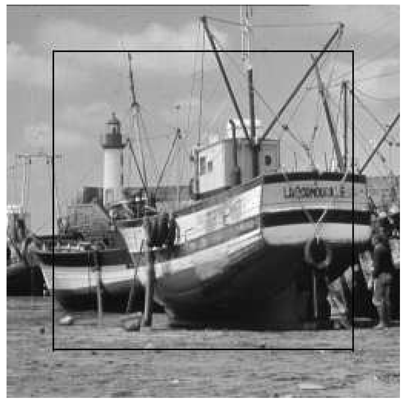
Collected images are available only in a finite region, the field of view (FOV), and the measured intensities near the boundary are affected by data which lie outside the FOV; see Figure 1 for an illustration.

Figure 1. Field of view. We see what is inside the square box.

Denoting by $\mathbf{g}$ and $\mathbf{f}$ the stack ordered vectors corresponding to the observed image and the true image, respectively, the discretization of (1) becomes

$$\mathbf{g}=K\mathbf{f}+\mathbf{\eta },$$

(2)

where the matrix K is of size $m^2\times k^2$, being m and k the dimensions (in pixels) of the original picture. The matrix K is often called the blurring matrix. When imposing proper Boundary Conditions (BCs), the matrix K becomes square $m^2\times m^2$ and in some cases, depending on the BCs and the symmetry of the PSF, it can be diagonalized by discrete trigonometric transforms. Indeed, specific BCs induce specific matrix structures that can be exploited to lessen the computational costs using fast algorithms. Of course, since BCs are artificially introduced, their advantages could come with drawbacks in terms of reconstruction accuracy, depending on the type of problem. The BCs approach forces a functional dependency between the elements of $\mathbf{f}$ external to the FOV and those internal to this area. If the BC model is not a good approximation of the real world outside the FOV, the reconstructed image can be severely affected by some unwanted artifacts near the boundary, called ringing effects; see, e.g., [1].

The choice of the different BCs can be driven by some additional knowledge on the true image and/or from the availability of fast transforms to diagonalize the matrix K within $O(m^{2}log\left(m\right))$ arithmetic operations. Indeed, the matrix-vector product can be always computed by the 2D FFT, after a proper padding of the image to convolve, (see, e.g., [2]), while the availability of fast transforms to diagonalize the matrix K depends on the BCs. Among the BCs present in the literature, we consider: Zero (Dirichlet), Periodic, Reflective and Anti-Reflective, but our approach can be extended to other BCs like, e.g., synthetic BCs [3] or high order BCs [4,5]. See Figure 2 for an illustration of the described BCs.

Figure 2. Examples of boundary conditions.

On the other hand, since Equation (2) is the product of the discretization of a compact operator, K is severely ill-conditioned and may be singular. Such linear systems are commonly referred to as linear discrete ill-posed problems; see, e.g., [6] for a discussion. Therefore a good approximation of $\mathbf{f}$ cannot be obtained from the algebraic solution (e.g., the least-square solution) of (2), but regularization methods are required. The basic idea of regularization is to replace the original ill-conditioned problem with a nearby well-conditioned problem, whose solution approximates the true solution. One of the popular regularization techniques is Tikhonov regularization and it amounts in solving

$$\underset{\mathbf{f}}{min}{\{\parallel K\mathbf{f}-\mathbf{g}\parallel }_2^2+{\mu \parallel \mathbf{f}\parallel }_2^2\},$$

(3)

where ${\parallel ·\parallel }_2$ denotes the vector 2-norm and $\mu >0$ is a regularization parameter to be chosen. The first term in (3) is usually refereed to as fidelity term and the second as regularization term. This translates into solving a linear problem for which many efficient methods have been developed for computing its solution and for estimating the regularizing parameter $\mu$, see [6]. This approach unfortunately comes with a drawback: the edges of restored images are usually over-smoothed. Therefore, nonlinear strategies have been employed, in order to overcome this unpleasant property, like total variation (TV) [7] and thresholding iterative methods [8,9]. That said, typically many nonlinear regularization methods have an inner step that apply a least-square regularization and therefore can benefit from strategies previously developed for such simpler model.

In the present paper, both the regularization strategies that we propose share two common ingredients: wavelet decomposition and ${\ell }_1$-norm minimization on the regularization term. This is motivated by the fact that the wavelet coefficients (under some basis) of most real images are usually very sparse. In particular, here we consider the tight frame systems used in [10,11,12], but the result can be easily extended to any framelet/wavelet system. Let $W^{*}$ be a wavelet or tight-frame synthesis operator ($W^{*}W=I$), the wavelets or tight-frame coefficients of the original image $\mathbf{f}$ are $\mathbf{x}$ such that

$$\mathbf{f}=W^{*}\mathbf{x},\hspace{1em}\mathrm{and} \mathrm{the} \mathrm{blurring} \mathrm{operator} \mathrm{becomes} A=K{W}^{*}.$$

Within this frame set, the model Equation (2) translates into

$$\mathbf{g}=A\mathbf{x}.$$

(4)

Recently, in [13], a new technique was proposed which directly applies a single preconditioning operator P to Equation (4). The new preconditioned system becomes

$$P\mathbf{g}=PA\mathbf{x}.$$

Combining this approach with a soft-thresholding technique such as the modified linearized Bregman splitting algorithm [14], in order to mimic the ${\ell }_1$-norm minimization, leads to the following preconditioned iterative scheme

$${\mathbf{x}}_{n+1}={\mathbf{x}}_n+\tau P(\mathbf{g}-A{\mathbf{S}}_{\mu }\left({\mathbf{x}}_n\right)),$$

where $\tau$ is a positive relaxation parameter and ${\mathbf{S}}_{\mu }(·)$ is the soft-thresholding function as defined in 6. Hereafter we will put $\tau =1$: this is justified by applying an implicit rescaling of the preconditioned system matrix $PA$.

The paper is organized as follows: in Section 2 we propose a generalization of an approximated iterative Tikhonov scheme that was firstly introduced in [15] and then developed and adapted into different settings in [16,17]. Here the preconditioner P takes the form

$$P=B^{*}{\left(B{B}^{*}+{\alpha }_n\mathsf{\Lambda }{\mathsf{\Lambda }}^{*}\right)}^{-1},$$

where B is an approximation of A, in the sense that $B=C{W}^{*}$ with C the discretization of the same problem (1) as the original blurring matrix K but imposing Periodic BCs. The operator $\mathsf{\Lambda }{\mathsf{\Lambda }}^{*}$ can be a function of $C{C}^{*}$ or the discretization of a differential operator. The method is nonstationary and the parameter ${\alpha }_n$ is computed by solving a nonlinear problem with a computational cost of $O\left(m^2\right)$. Related work on this kind of preconditioner can be found in [18,19,20]. In Section 3 we define a class of preconditioners P endowed with the same structure of the system matrix A, as initially proposed in [21] and then further developed in [22]. It is called structure preserving reblurring preconditioning strategy and we combine it with the generalized regularization filtering approach of the preceding Section 2. The idea is to preserve both the informations carried over by the spectra of the operator A and the structure itself of the operator induced by the best fitting BCs. Section 4 contains a selection of significant numerical examples which confirm the robustness and quality of the proposed regularization schemes. Section 5 provides a summary of the techniques presented in this work and draws some conclusions. Finally, in Appendix A are provided proofs of convergence and regularization properties of the proposed algorithms.

2. Preconditioned Iterated Soft-Thresholding Tikhonov with General Regularizing Operator

2.1. Preliminary Definitions

Before proceeding further, let us introduce here some definitions and notations that will be used in the forthcoming sections. We consider

$$K:\left({\mathbb{R}}^{m^2},\parallel ·\parallel \right)\to \left({\mathbb{R}}^{m^2},\parallel ·\parallel \right)$$

to be the discretization of a compact linear operator

$$\mathbf{g}=K\mathbf{f},$$

where the Euclidean 2-norm $\parallel ·\parallel$ is induced by the standard Euclidean inner product

$${⟨{\mathbf{f}}^{\left(1\right)},{\mathbf{f}}^{\left(2\right)}⟩}_{{\mathbb{R}}^{m^2}}=\sum _{j=1}^{m^2}{f}_j^{\left(1\right)}{f}_j^{\left(2\right)}.$$

Hereafter, we will specify the vector space where the inner product $⟨·,·⟩$ acts only whenever it is necessary for disambiguation. The analysis that will follow in the next sections will be performed generally on a perturbed data ${\mathbf{g}}^{\delta }$, namely

$${\mathbf{g}}^{\delta }=K\mathbf{f},$$

with ${\mathbf{g}}^{\delta }=\mathbf{g}+\mathbf{\eta }$, and where $\mathbf{\eta }$ is a noise vector such that $\parallel \mathbf{\eta }\parallel =\delta$, $\delta$ is called the noise level.

Let

$$C:\left({\mathbb{R}}^{m^2},\parallel ·\parallel \right)\to \left({\mathbb{R}}^{m^2},\parallel ·\parallel \right)$$

be the discretization of a compact linear operator that approximates K, in a sense that will be specified later. Let

$$W:\left({\mathbb{R}}^{m^2},\parallel ·\parallel \right)\to \left({\mathbb{R}}^s,\parallel ·\parallel \right)$$

be such that

$$W^{*}W=I,$$

where $W^{*}:{\mathbb{R}}^s\to {\mathbb{R}}^{m^2}$ indicates the adjoint operator of W, i.e., ${⟨W\mathbf{f},\mathbf{u}⟩}_{{\mathbb{R}}^s}={⟨\mathbf{f},W^{*}\mathbf{u}⟩}_{{\mathbb{R}}^{m^2}}$ for each pair $\mathbf{f}\in {\mathbb{R}}^{m^2},\mathbf{u}\in {\mathbb{R}}^s$. We define

$$\mathbf{x}=W\mathbf{f},\hspace{1em}A=K{W}^{*},\hspace{1em}B=C{W}^{*}.$$

Let us introduce the following matrix norm. Given a generic linear operator

$$L:\left({\mathbb{R}}^s,{\parallel ·\parallel }_{\infty }\right)\to \left({\mathbb{R}}^{m^2},\parallel ·\parallel \right),$$

where ${\parallel ·\parallel }_{\infty }$ is the sup norm, let us define the matrix norm $\left|\left|\left|·\right|\right|\right|$ as

$$\left|\left|\left|L\right|\right|\right|:=\underset{{\parallel \mathbf{x}\parallel }_{\infty }\equiv 1}{sup}{\parallel L\mathbf{x}\parallel }_2.$$

(5)

Finally, let $\mu \ge 0$ and let ${\mathbf{S}}_{\mu }:{\mathbb{R}}^s\to {\mathbb{R}}^s$ be such that

$${\left[{\mathbf{S}}_{\mu }\left(\mathbf{u}\right)\right]}_i=S_{\mu }\left(u_i\right),$$

(6)

with $S_{\mu }$ the soft-thresholding function

$$S_{\mu }\left(u_i\right)=\mathrm{sgn}\left(u_i\right)max\left\{|u_i|-\mu ,0\right\}.$$

2.2. General Regularization Operator as $h\left(C{C}^{*}\right)$

Let $h:[0,\parallel C{C}^{*}{\parallel }^2]\to \mathbb{R}$ be a continuous function such that

$$0<c_1\le h\left({\sigma }^2\right)\le c_2,$$

where $c_1,c_2$ are positive constants, and define $c:=c_1/c_2$. By the continuity of h and by well-known facts from functional analysis [23] we can write $h\left(C{C}^{*}\right)$ as the operator defined by

$$h\left(C{C}^{*}\right)\left[\mathbf{f}\right]:=\int h\left({\sigma }^2\right)d{E}_{{\sigma }^2}\left(\mathbf{f}\right)=\sum _{k=1}^{\infty }h\left({\sigma }_k^2\right)⟨\mathbf{f},{\mathbf{u}}_k⟩{\mathbf{u}}_k,$$

where ${\left\{E_{{\sigma }^2}\right\}}_{{\sigma }^2\in \sigma \left(C{C}^{*}\right)}$ is the spectral decomposition of a (generic) self-adjoint operator $C{C}^{*}$ and ${\left({\sigma }_k,{\mathbf{v}}_k,{\mathbf{u}}_k\right)}_{k\in \mathbb{N}}$ is the singular value expansion of C. We summarize the computations in Algorithm 1.

Algorithm 1${\mathrm{PISTA}}_h$

Fix ${\mathbf{z}}^0\in {\mathbb{R}}^s$, $\delta >0$ and set ${\mathbf{x}}^0={\mathbf{S}}_{\mu }\left({\mathbf{z}}^0\right)$, ${\mathbf{r}}^0=\mathbf{g}-A{\mathbf{x}}^0$. Set $\rho \in (0,c/2)$ and $q\in (2\rho ,c)$. Compute $\tau =\frac{1+2\rho }{c-2\rho }$ and ${\mathbf{r}}^n=\mathbf{g}-A{\mathbf{x}}^n$. while$\parallel {\mathbf{r}}^n\parallel >\tau \delta$ do  Compute ${\tau }_n:=\parallel {\mathbf{r}}^n\parallel /\delta$.  Compute $q_n:=max\{q,2\rho +(1+\rho )/{\tau }_n\}$.  Compute ${\alpha }_n$ such that $$\begin{array}{c}\hfill {\alpha }_n\parallel {(C{C}^{*}+{\alpha }_{n}h\left(C{C}^{*}\right))}^{-1}{\mathbf{r}}^n\parallel =\frac{q_n}{c_1}\parallel {\mathbf{r}}^n\parallel .\end{array}$$ (7) Compute $${\mathbf{h}}^n=W{C}^{*}{(C{C}^{*}+{\alpha }_{n}h\left(C{C}^{*}\right))}^{-1}{\mathbf{r}}^n.$$ (8) Compute $$\left\{\begin{array}{c}{\mathbf{z}}^{n+1}={\mathbf{z}}^n+{\mathbf{h}}^n,\hfill \\ {\mathbf{x}}^{n+1}={\mathbf{S}}_{\mu }\left({\mathbf{z}}^{n+1}\right).\hfill \end{array}\right.$$

A rigorous and full detailed analysis of the preceding algorithm will be performed in Appendix A. In order to prove all the desired properties we will need a couple of assumptions on the operators K, C, and on the parameter $\mu$, that we present here below.

Assumption 1.

$$\parallel \left(C-K\right)\mathbf{f}\parallel \le \rho \parallel K\mathbf{f}\parallel ,\hspace{1em}\forall \mathbf{f}\in {\mathbb{R}}^{m^2},$$

(9a)

and

$$\mu \le \frac{\rho \delta }{\left|\left|\left|B\right|\right|\right|},$$

(9b)

with a fixed $0<\rho <c/2$, where $\delta =\parallel \mathbf{\eta }\parallel$ is the noise level and where $\left|\left|\left|·\right|\right|\right|$ is the operator norm defined in (5).

Let us observe that Equation (9a) translates into

$$\parallel (B-A)\mathbf{u}\parallel \le \rho \parallel A\mathbf{u}\parallel ,\hspace{1em}\forall \mathbf{u}\in {\mathbb{R}}^s.$$

(10)

Let us spread some light on the preceding conditions. Assumption (9a), or equivalently (10), is a strong assumption. It may be hard to satisfy it for every specific problem, as it implies

$$\left(1-\rho \right)\parallel K\mathbf{v}\parallel \le \parallel C\mathbf{v}\parallel \le \left(1+\rho \right)\parallel K\mathbf{v}\parallel \hspace{1em}\mathrm{for} \mathrm{all}\mathbf{v}\in {\mathbb{R}}^{m^2},$$

or equivalently

$$\left(1-\rho \right)\parallel A\mathbf{u}\parallel \le \parallel B\mathbf{u}\parallel \le \left(1+\rho \right)\parallel A\mathbf{u}\parallel \hspace{1em}\mathrm{for} \mathrm{all}\mathbf{u}\in {\mathbb{R}}^s,$$

(11)

that is, K and C are spectrally equivalent. Nevertheless, in image deblurring the boundary conditions have a very local effect, i.e., the approximation error $C-K$ can be decomposed as

$$C-K=E+R,$$

where E is a matrix of small norm (and the zero matrix if the PSF is compactly supported), and R is a matrix of small rank, compared to the dimension of the problem. This suggests that Assumption (9a) needs to be satisfied only in a relatively small subspace, supposedly being a zero measure subspace. In particular only for every ${\mathbf{e}}_{\delta }^n$, with $n\ge N$ and N fixed, such that Proposition A1 in Appendix A could hold. All the numerical experiments are consistent with this observation but for a deeper understanding and a full treatment of this aspect we refer the reader to ([15], Section 4).

On the other hand instead, Assumption (9b) is quite natural. It is indeed equivalent to require that

$$\parallel B\left(\mathbf{u}-{\mathbf{S}}_{\mu }\left(\mathbf{u}\right)\right)\parallel \le \rho \delta$$

that is, the soft-thresholding parameter $\mu =\mu \left(\delta \right)$ is continuously noise-dependent and it holds that $\mu \left(\delta \right)\to 0$ as $\delta \to 0$.

2.3. General Regularization Operator as $\mathsf{\Lambda }{\mathsf{\Lambda }}^{*}$

In image deblurring, in order to better preserve the edges of the reconstructed solution, it is usually introduced a differential operator $\mathsf{\Lambda }{\mathsf{\Lambda }}^{*}$, where $\mathsf{\Lambda }:\mathcal{X}\to \mathcal{Y}$ is chosen as a first or second order differential operator which holds in its kernel all these functions which posses the key features of the true solution that we wish to preserve. In particular, since we are interested to recover the edges and curves of discontinuities of the true image, it is a common choice to rely on the Laplace operator with Neumann BCs, see [24]. In these recent papers [25,26], observing the spectral distribution of the Laplacian, it was proposed to substitute $\mathsf{\Lambda }{\mathsf{\Lambda }}^{*}$ with

$$h\left(C{C}^{*}\right)={\left(I-\frac{C{C}^{*}}{\parallel C{C}^{*}\parallel }\right)}^j,$$

with $j\in \mathbb{N}$.

Adding some new assumptions, we propose a modified version of the preceding Algorithm 1 that can take into account directly the operator $\mathsf{\Lambda }$.

Assumption 2.

$$\mathrm{Ker}\left(K\right)\cap \mathrm{Ker}\left(\mathsf{\Lambda }\right)=\left\{0\right\};$$

$$C_{\left|\mathrm{Ker}\right(\mathsf{\Lambda })}=K_{\left|\mathrm{Ker}\right(\mathsf{\Lambda })};$$

$$C and \mathsf{\Lambda } are diagonalized by the same unitary transform.$$

We summarize the computations in Algorithm 2.

Algorithm 2${\mathrm{PISTA}}_{\mathsf{\Lambda }}$

Fix ${\mathbf{z}}^0\in {\mathbb{R}}^s$, $\delta >0$ and set ${\mathbf{x}}^0={\mathbf{S}}_{\mu }\left({\mathbf{z}}^0\right)$, ${\mathbf{r}}^0=\mathbf{g}-A{\mathbf{x}}^0$. Set $\rho \in (0,1/2)$ and $q\in (2\rho ,1)$. Compute $\tau =\frac{1+2\rho }{1-2\rho }$ and ${\mathbf{r}}^n=\mathbf{g}-A{\mathbf{x}}^n$. while  $\parallel {\mathbf{r}}^n\parallel >\tau \delta$ do  Compute ${\tau }_n:=\parallel {\mathbf{r}}^n\parallel /\delta$.  Compute $q_n:=max\{q,2\rho +(1+\rho )/{\tau }_n\}$.  Compute ${\alpha }_n$ such that $$\begin{array}{c}\hfill {\alpha }_n\parallel {(C{C}^{*}+{\alpha }_n\mathsf{\Lambda }{\mathsf{\Lambda }}^{*})}^{-1}{\mathbf{r}}^n\parallel =q_n\parallel {\mathbf{r}}^n\parallel .\end{array}$$ Compute $${\mathbf{h}}^n=W{C}^{*}{(C{C}^{*}+{\alpha }_n\mathsf{\Lambda }{\mathsf{\Lambda }}^{*})}^{-1}{\mathbf{r}}^n.$$ (12) Compute $$\left\{\begin{array}{c}{\mathbf{z}}^{n+1}={\mathbf{z}}^n+{\alpha }_n{\mathbf{h}}^n,\hfill \\ {\mathbf{x}}^{n+1}={\mathbf{S}}_{\mu }\left({\mathbf{z}}^{n+1}\right).\hfill \end{array}\right.$$

We skip all the proofs of convergence since they can be recovered easily adapting the proofs in Appendix A with ([16], Section 4).

3. Structured PISTA with General Regularizing Operator

The structured case is a generalization of what was developed in [21,22], merging these ideas with the general approach described in Section 2. We skip some details since they can be easily recovered from the aforementioned papers.

The blurring matrix K is made by two parts: the PSF and the BCs inherited by the discretization. Different types of structured matrices are given rise by this latter choice. Without loosing generality and for the sake of simplicity, we consider a square PSF $H_{\kappa }\in {\mathbb{R}}^{k\times k}$ and we suppose that the center of the PSF is known.

Consider the pixels ${\kappa }_{i,j}$ of the PSF, we can define the following generating function $\kappa :{\mathbb{R}}^2\to \mathbb{C}$

$$\kappa (x_1,x_2)=\sum _{i,j=-m+1}^{m-1}{\kappa }_{i,j}{\mathrm{e}}^{\widehat{ı}(i{x}_1+j{x}_2)},$$

(13)

where ${\widehat{ı}}^2=-1$ and we assumed that ${\kappa }_{i,j}=0$ if the entry $\left({\kappa }_{i,j}\right)$ does not belong to $H_{\kappa }$ [5]. Observe that ${\kappa }_{j,j}$ can be seen as the Fourier coefficients of $\kappa \in \mathrm{span}\{{\mathrm{e}}^{\widehat{ı}(i{x}_1+j{x}_2)},i,j=-k,\cdots ,k\}$, so that the same information is contained in the generating function $\kappa$ and in $H_{\kappa }$.

Summarizing the notation that we set in the Introduction about the BCs, we have

$$\begin{array}{cc}\mathrm{Zero} \mathrm{BCs}:\hfill & K={\mathcal{T}}_m\left(\kappa \right),\hfill \\ \mathrm{Periodic} \mathrm{BCs}:\hfill & K={\mathcal{C}}_m\left(\kappa \right)={\mathcal{T}}_m\left(\kappa \right)+{\mathcal{B}}_m^{\mathcal{C}}\left(\kappa \right),\hfill \\ \mathrm{Reflective} \mathrm{BCs}:\hfill & K={\mathcal{R}}_m\left(\kappa \right)={\mathcal{T}}_m\left(\kappa \right)+{\mathcal{B}}_m^{\mathcal{R}}\left(\kappa \right),\hfill \\ \mathrm{Anti}\text{-}\mathrm{Reflective} \mathrm{BCs}:\hfill & K={\mathcal{AR}}_m\left(\kappa \right)={\mathcal{T}}_m\left(\kappa \right)+{\mathcal{B}}_m^{\mathcal{AR}}\left(\kappa \right).\hfill \end{array}$$

We notice that, since the continuous operator is shift-invariant, in all these four cases K has a Toeplitz structure ${\mathcal{T}}_m\left(\kappa \right)$ which depends on $\kappa$ plus a correction term ${\mathcal{B}}_m^{\mathcal{X}}\left(\kappa \right),\mathcal{X}=\mathcal{C},\mathcal{R},\mathcal{AR}$ which depends on the chosen BCs.

In conclusion, we employ the unified notation $K={\mathcal{M}}_m\left(\kappa \right)$, where $\mathcal{M}(·)$ can be any of the classes of matrices just introduced (i.e., $\mathcal{T}$, $\mathcal{C}$, $\mathcal{R}$, $\mathcal{AR}$). With this notation we wish to highlight the two crucial elements that determine K: the blurring phenomenon associated with the PSF described by $\kappa$ and the chosen BCs represented by $\mathcal{M}$.

Given the generating function $\kappa$ (13) associated to the PSF $H_{\kappa }$, let us compute the eigenvalues $u_{i,j}$ of the corresponding BCCB matrix ${\mathcal{C}}_m\left(\kappa \right):=C$ by means of the 2D-FFT, where $i,j=0,\cdots ,m-1$. Fix a regularizing (differential) operator $\mathsf{\Lambda }{\mathsf{\Lambda }}^{*}$ as in Section 2, and suppose that the Assumptions 1 and 2 hold. The differential operator can be of the form $\mathsf{\Lambda }{\mathsf{\Lambda }}^{*}=h\left(C{C}^{*}\right)$, as in Algorithm 1 as well. Let now

$$v_{i,j}=\frac{{\overline{u}}_{i,j}}{|u_{i,j}{|}^2+{\alpha }_n{\left|{\sigma }_{i,j}\right|}^2},\hspace{1em}\left({\overline{u}}_{i,j}\mathrm{the} \mathrm{complex} \mathrm{conjugate} \mathrm{of} u_{i,j}\right)$$

be the new eigenvalues after the application of the Tikhonov filter to $u_{i,j}$, where ${\sigma }_{i,j}$ are the eigenvalues (singular values) of $\mathsf{\Lambda }$ and ${\alpha }_n$ is computed as in Algorithms 1 and 2. Let us compute now the coefficients ${\widehat{\kappa }}_{i,j}$ of

$$\widehat{\kappa }(x_1,x_2)=\sum _{i,j=-m+1}^{m-1}{\widehat{\kappa }}_{i,j}{\mathrm{e}}^{\widehat{ı}({\mathrm{ix}}_1+{\mathrm{jx}}_2)}$$

(14)

by means of the 2D-iFFT and, finally, let us define

$$P={\mathcal{M}}_m\left(\widehat{\kappa }\right),$$

where $\mathcal{M}(·)$ corresponds to the most fitting BCs for the model problem (1).

We are now ready to formulate the last method whose computation are reported in Algorithm 3.

Algorithm 3${\mathrm{Struct}\text{-}\mathrm{PISTA}}_{\mathsf{\Lambda }}$

Fix $H_{\kappa }$, BCs, $\mathsf{\Lambda }$. Set $C={\mathcal{C}}_m\left(\kappa \right)$. Get ${\left\{u_{i,j}\right\}}_{i,j=0}^{n-1}$ by computing an FFT of $H_{\kappa }$. Fix ${\mathbf{z}}^0\in {\mathbb{R}}^s$, $\delta >0$ and set ${\mathbf{x}}^0={\mathbf{S}}_{\mu }\left({\mathbf{z}}^0\right)$, ${\mathbf{r}}^0=\mathbf{g}-K{\mathbf{x}}^0$. Set $\rho \in (0,1/2)$ and $q\in (2\rho ,1)$. Compute $\tau =\frac{1+2\rho }{1-2\rho }$ and ${\mathbf{r}}^n=\mathbf{g}-K{\mathbf{x}}^n$. while  $\parallel {\mathbf{r}}^n\parallel >\tau \delta$ do  Compute ${\tau }_n:=\parallel {\mathbf{r}}^n\parallel /\delta$.  Compute $q_n:=max\{q,2\rho +(1+\rho )/{\tau }_n\}$.  Compute ${\alpha }_n$ such that $$\begin{array}{c}\hfill {\alpha }_n\parallel {(C{C}^{*}+{\alpha }_n\mathsf{\Lambda }{\mathsf{\Lambda }}^{*})}^{-1}{\mathbf{r}}^n\parallel =q_n\parallel {\mathbf{r}}^n\parallel .\end{array}$$ Compute $v_{i,j}=\frac{{\overline{u}}_{i,j}}{{\left|u_{i,j}\right|}^2+{\alpha }_n{\left|{\sigma }_{i,j}\right|}^2}$. Get the mask $\tilde{H}$ of the coefficients ${\widehat{\kappa }}_{i,j}$ of $\widehat{\kappa }$ of (14) by computing an IFFT of ${\left\{v_{i,j}\right\}}_{i,j=0}^{m-1}$. Generate the matrix $P:={\mathcal{M}}_m\left(\widehat{\kappa }\right)$ from the coefficient mask $\tilde{H}$ and BCs. Compute $${\mathbf{h}}^n=P{\mathbf{r}}^n.$$ (15) Compute $$\left\{\begin{array}{c}{\mathbf{z}}^{n+1}={\mathbf{z}}^n+{\mathbf{h}}^n,\hfill \\ {\mathbf{x}}^{n+1}={\mathbf{S}}_{\mu }\left({\mathbf{z}}^{n+1}\right).\hfill \end{array}\right.$$

In the case that $\mathsf{\Lambda }{\mathsf{\Lambda }}^{*}=h\left(C{C}^{*}\right)$, then the algorithm is modified in the following way:

$$\rho \in (0,c/2),\hspace{1em}q\in (2\rho ,c),\hspace{1em}{\alpha }_n\parallel {(C{C}^{*}+{\alpha }_n\mathsf{\Lambda }{\mathsf{\Lambda }}^{*})}^{-1}{\mathbf{r}}^n\parallel =\frac{q_n}{c_1}\parallel {\mathbf{r}}^n\parallel$$

where $0<c_1\le h\left({\sigma }^2\right)\le c_2$, $c:=c_1/c_2$. We will denote this version by ${\mathrm{Struct}\text{-}\mathrm{PISTA}}_h$. We will not provide a direct proof of convergence for this last algorithm. Let us just observe that the difference between (15) and (12)–(8) is just a correction of small rank and small norm.

4. Numerical Experiments

We now compare the proposed algorithms with some methods from the literature. In particular, we consider the AIT-GP algorithm described in [16] and the ISTA algorithm described in [8]. The AIT-GP method can be seen as Algorithm 2 with $\mu =0$, while the ISTA algorithm is equivalent to iterations of Algorithm 2 without the preconditioner. These comparisons allow us to show how the quality of the reconstructed solution is improved by the presence of both the soft-thresholding and the preconditioner.

The ISTA method and our proposals require the selection of a regularization parameter. For all these methods we select the parameter that minimizes the relative restoration error (RRE) defined by

$$\mathrm{RRE}\left(\mathbf{f}\right)=\frac{\parallel \mathbf{f}-{\mathbf{f}}_{\mathrm{true}}\parallel }{\parallel {\mathbf{f}}_{\mathrm{true}}\parallel }.$$

For the comparison of the algorithms we consider the Peak Signal to Noise Ratio (PSNR) defined by    

$$\mathrm{PSNR}\left(\mathbf{f}\right)=20{log}_{10}\left(\frac{mM}{\parallel \mathbf{f}-{\mathbf{f}}_{\mathrm{true}\parallel }}\right),$$

where $m^2$ is the the number of elements of $\mathbf{f}$ and M denotes the maximum value of ${\mathbf{f}}_{\mathrm{true}}$. Moreover, we consider the Structure Similarity index (SSIM); the definition of the SSIM is involved, here we recall that this index measures how accurately the computed approximation is able to reconstruct the overall structure of the image. The higher the value of the SSIM the better the reconstruction is, and the maximum value achievable is 1; see [27] for a precise definition of the SSIM.

We now describe how we construct the operator W. We use the tight frames determined by linear B-splines; see, e.g., [28]. For one-dimensional problems they are composed by a low-pass filter $W_0\in {\mathbb{R}}^{m\times m}$ and two high-pass filters $W_1\in {\mathbb{R}}^{m\times m}$ and $W_2\in {\mathbb{R}}^{m\times m}$. These filters are determined by the masks are given by

$$u^{\left(0\right)}=\frac{1}{4}[1,2,1],\hspace{1em}{u}^{\left(1\right)}=\frac{\sqrt{2}}{4}[1,0,-1],\hspace{1em}{u}^{\left(2\right)}=\frac{1}{4}[-1,2,-1].$$

Imposing reflexive boundary conditions we determine the analysis operator W so that $W^{*}W=I$. Define the matrices

$$W_0=\frac{1}{4}\left(\begin{array}{ccccc}3& 1& 0& \cdots & 0\\ 1& 2& 1\\ \hspace{1em}& \ddots & \ddots & \ddots \\ \hspace{1em}& \hspace{1em}& 1& 2& 1\\ 0& \cdots & 0& 1& 3\end{array}\right),\hspace{1em}{W}_1=\frac{\sqrt{2}}{4}\left(\begin{array}{ccccc}-1& 1& 0& \cdots & 0\\ -1& 0& 1\\ \hspace{1em}& \ddots & \ddots & \ddots \\ \hspace{1em}& \hspace{1em}& -1& 0& 1\\ 0& \cdots & 0& -1& 1\end{array}\right),$$

and

$$W_2=\frac{1}{4}\left(\begin{array}{ccccc}1& -1& 0& \cdots & 0\\ -1& 2& -1\\ \hspace{1em}& \ddots & \ddots & \ddots \\ \hspace{1em}& \hspace{1em}& -1& 2& -1\\ 0& \cdots & 0& -1& 1\end{array}\right).$$

Then the operator W is defined by

$$W=\left(\begin{array}{c}{W}_0\\ W_1\\ W_2\end{array}\right).$$

To construct the two-dimensional framelet analysis operator we use the tensor products

$$W_{i,j}=W_i\otimes W_j,\hspace{1em}i,j=0,1,2.$$

The matrix $W_{00}$ is a low-pass filter; all the other matrices $W_{ij}$ contain at least one high-pass filter. The analysis operator is given by

$$W=\left[\begin{array}{c}{W}_{00}\\ W_{01}\\ ⋮\\ W_{22}\end{array}\right].$$

In ${\mathrm{PISTA}}_h$, following [26], we set

$$h\left(x\right)={\left(1-\frac{x}{{\parallel A\parallel }^2}\right)}^4+{10}^{-15}.$$

All the computations were performed on MATLAB R2018b running on a laptop with an Intel i7-8750H @ 2.20 GHz CPU and 16 GB of RAM.

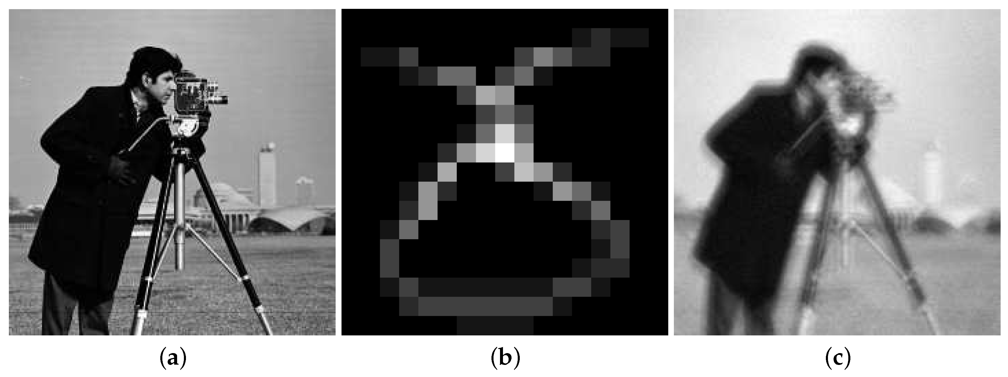
4.1. Cameraman

We first considered the cameraman image in Figure 3a and we blurred it with the non-symmetric PSF in Figure 3b. We then added $2\%$ white Gaussian noise obtaining the blurred and noisy image in Figure 3c. Note that we cropped the boundaries of the image to simulate real data; see [1] for more details. Since the image was generic we imposed reflexive BCs.

Figure 3. Cameraman test problem: (a) True image ($238\times 238$ pixels), (b) point spread function (PSF) ($17\times 17$ pixels), (c) Blurred and noisy image with $2\%$ of white Gaussian noise ($238\times 238$ pixels).

In Table 1 we report the results obtained with the different methods. We can observe that ${\mathrm{Struct}\text{-}\mathrm{PISTA}}_h$ provided the best reconstruction of all considered algorithms. Moreover, we can observe that, in general, the introduction of the structured preconditioner improved the quality of the reconstructed solutions, especially in terms of SSIM. From the visual inspection of the reconstructions in Figure 4 we can observe that the introduction of the structured preconditioner allowed us to evidently reduce the boundary artifacts as well as avoid the amplification of the noise.

Table 1. Comparison of the quality of the reconstructions for all considered examples. We highlight in boldface the best result.

Example	Method	RRE	PSNR	SSIM
Cameraman	AIT-GP	$0.111024$	$24.7798$	$0.729095$
	ISTA	$0.090921$	$26.5149$	$0.763217$
	${\mathrm{PISTA}}_h$	$0.096558$	$25.9924$	$0.790363$
	${\mathrm{PISTA}}_{\mathsf{\Lambda }}$	$0.094853$	$26.1471$	$0.795061$
	${\mathrm{Struct}\text{-}\mathrm{PISTA}}_h$	$\mathbf{0.088796}$	$\mathbf{26.7203}$	$\mathbf{0.840145}$
	${\mathrm{Struct}\text{-}\mathrm{PISTA}}_{\mathsf{\Lambda }}$	$0.090182$	$26.5857$	$0.834532$
Grain	AIT-GP	$0.183796$	$25.9571$	$0.731407$
	ISTA	$\mathbf{0.160655}$	$\mathbf{27.1259}$	$0.845816$
	${\mathrm{PISTA}}_h$	$0.195516$	$25.4202$	$0.737254$
	${\mathrm{PISTA}}_{\mathsf{\Lambda }}$	$0.181727$	$26.0554$	$0.748582$
	${\mathrm{Struct}\text{-}\mathrm{PISTA}}_h$	$0.161715$	$27.0688$	$\mathbf{0.859284}$
	${\mathrm{Struct}\text{-}\mathrm{PISTA}}_{\mathsf{\Lambda }}$	$0.168472$	$26.7133$	$0.830990$
Satellite	AIT-GP	$0.222783$	$26.6708$	$0.742416$
	ISTA	$0.286179$	$24.4956$	$0.657111$
	${\mathrm{PISTA}}_h$	$0.192146$	$27.9558$	$0.928584$
	${\mathrm{PISTA}}_{\mathsf{\Lambda }}$	$0.193730$	$27.8844$	$0.916993$
	${\mathrm{Struct}\text{-}\mathrm{PISTA}}_h$	$\mathbf{0.187970}$	$\mathbf{28.1466}$	$\mathbf{0.934876}$
	${\mathrm{Struct}\text{-}\mathrm{PISTA}}_{\mathsf{\Lambda }}$	$0.189147$	$28.0924$	$0.924931$

Figure 4. Cameraman test problem reconstructions: (a) ISTA, (b) ${\mathrm{PISTA}}_h$, (c) ${\mathrm{Struct}\text{-}\mathrm{PISTA}}_h$.

4.2. Grain

We now considered the grain image in Figure 5a and blurred it with the PSF, obtained by the superposition of two motions PSF, in Figure 5b. After adding $3\%$ of white Gaussian noise and cropping the boundaries we obtained the blurred and noisy image in Figure 5c. According to the nature of the image we used reflexive bc’s.

Figure 5. Grain test problem: (a) True image ($246\times 246$ pixels), (b) PSF ($9\times 9$ pixels), (c) Blurred and noisy image with $3\%$ of white Gaussian noise ($246\times 246$ pixels).

Again in Table 1 we report all the results obtained with the considered methods. In this case ISTA provided the best reconstruction in terms of RRE and PSNR. However, ${\mathrm{Struct}\text{-}\mathrm{PISTA}}_h$ provided the best reconstruction terms of SSIM and very similar results in term of PSNR and RRE. In Figure 6 we report some of the reconstructed solution. From the visual inspection of these reconstruction we can see that the introduction of the structured preconditioner reduced the ringing and boundary effects in the computed solutions.

Figure 6. Grain test problem reconstructions: (a) ISTA, (b) ${\mathrm{PISTA}}_{\mathsf{\Lambda }}$, (c) ${\mathrm{Struct}\text{-}\mathrm{PISTA}}_{\mathsf{\Lambda }}$.

4.3. Satellite

Our final example is the atmosphericBlur30 from the MATLAB toolbox RestoreTools [2]. The true image, PSF, and blurred and noisy image are reported in Figure 7a–c, respectively. Since we knew the true image we could estimate the noise level in the image, which was approximately $1\%$. Since this was an astronomical image we imposed zero bc’s.

Figure 7. Satellite test problem: (a) True image ($256\times 256$ pixels), (b) PSF ($256\times 256$ pixels), (c) Blurred and noisy image with ≈$1\%$ of white Gaussian noise ($256\times 256$ pixels).

From the comparison of the computed results in Table 1 we can see that the ${\mathrm{Struct}\text{-}\mathrm{PISTA}}_h$ method provided the best reconstruction among all considered methods. We can observe that, in this particular example, ISTA provided a very low quality reconstruction both in term of RRE and SSIM. We report in Figure 8 some reconstructions. From the visual inspection of the computed solutions we can observe that both the approximations obtained with ${\mathrm{PISTA}}_h$ and ${\mathrm{Struct}\text{-}\mathrm{PISTA}}_h$ did not present heavy ringing effects, while the reconstruction obtained by AIT-GP presented very heavy ringing around the “arms” of the satellite. This allowed us to show the benefits of introducing the soft-thresholding into the AIT-GP method.

Figure 8. Satellite test problem reconstructions: (a) AIT-GP, (b) ${\mathrm{PISTA}}_h$, (c) ${\mathrm{Struct}\text{-}\mathrm{PISTA}}_h$.

5. Conclusions

This work develops further and brings together all the techniques studied in [16,17,21,22,29]. The idea is to combine thresholding iterative methods, an approximate Tikhonov regularization scheme depending on a general (differential) operator and a structure preserving approach, with the main goal in mind to reduce the boundary artifacts which appear in the resulting de-blurred image when imposing artificial boundary conditions. The numerical results are promising and show improvements with respect to known state-of-the-art deblurring algorithms. There are still open problems, mainly concerning the theoretical assumptions and convergence proofs which will be furtherly investigated in future works.

References

- Hansen, P.C.; Nagy, J.G.; O’leary, D.P. Deblurring Images: Matrices, Spectra, and Filtering; Siam: Philadelphia, PA, USA, 2006; Volume 3. [Google Scholar]
- Nagy, J.G.; Palmer, K.; Perrone, L. Iterative methods for image deblurring: A Matlab object-oriented approach. Numer. Algorithms 2004, 36, 73–93. [Google Scholar] [CrossRef]
- Almeida, M.S.; Figueiredo, M. Deconvolving images with unknown boundaries using the alternating direction method of multipliers. IEEE Trans. Image Process. 2013, 22, 3074–3086. [Google Scholar] [CrossRef] [PubMed]
- Dell’Acqua, P. A note on Taylor boundary conditions for accurate image restoration. Adv. Comput. Math. 2017, 43, 1283–1304. [Google Scholar] [CrossRef]
- Donatelli, M. Fast transforms for high order boundary conditions in deconvolution problems. BIT Numer. Math. 2010, 50, 559–576. [Google Scholar] [CrossRef]
- Hanke, M.; Hansen, P.C. Regularization methods for large-scale problems. Surv. Math. Ind. 1993, 3, 253–315. [Google Scholar]
- Rudin, L.I.; Osher, S.; Fatemi, E. Nonlinear total variation based noise removal algorithms. Physica D 1992, 60, 259–268. [Google Scholar] [CrossRef]
- Daubechies, I.; Defrise, M.; De Mol, C. An iterative thresholding algorithm for linear inverse problems with a sparsity constraint. Commun. Pure Appl. Math. 2004, 57, 1413–1457. [Google Scholar] [CrossRef]
- Figueiredo, M.A.; Nowak, R.D. An EM algorithm for wavelet-based image restoration. IEEE Trans. Image Process. 2003, 12, 906–916. [Google Scholar] [CrossRef]
- Chan, R.H.; Chan, T.F.; Shen, L.; Shen, Z. Wavelet algorithms for high-resolution image reconstruction. SIAM J. Sci. Comput. 2003, 24, 1408–1432. [Google Scholar] [CrossRef]
- Cai, J.F.; Osher, S.; Shen, Z. Linearized Bregman iterations for frame-based image deblurring. SIAM J. Imag. Sci. 2009, 2, 226–252. [Google Scholar] [CrossRef]
- Cai, J.F.; Osher, S.; Shen, Z. Split Bregman methods and frame based image restoration. Multiscale Model. Simul. 2010, 8, 337–369. [Google Scholar] [CrossRef]
- Dell’Acqua, P.; Donatelli, M.; Estatico, C. Preconditioners for image restoration by reblurring techniques. J. Comput. Appl. Math. 2014, 272, 313–333. [Google Scholar] [CrossRef]
- Yin, W.; Osher, S.; Goldfarb, D.; Darbon, J. Bregman iterative algorithms for ℓ1-minimization with applications to compressed sensing. SIAM J. Imag. Sci. 2008, 1, 143–168. [Google Scholar] [CrossRef]
- Donatelli, M.; Hanke, M. Fast nonstationary preconditioned iterative methods for ill-posed problems, with application to image deblurring. Inverse Probl. 2013, 29, 095008. [Google Scholar] [CrossRef]
- Buccini, A. Regularizing preconditioners by non-stationary iterated Tikhonov with general penalty term. Appl. Numer. Math. 2017, 116, 64–81. [Google Scholar] [CrossRef]
- Cai, Y.; Donatelli, M.; Bianchi, D.; Huang, T.Z. Regularization preconditioners for frame-based image deblurring with reduced boundary artifacts. SIAM J. Sci. Comput. 2016, 38, B164–B189. [Google Scholar] [CrossRef]
- Buccini, A.; Donatelli, M.; Reichel, L. Iterated Tikhonov regularization with a general penalty term. Numer. Linear Algebra Appl. 2017, 24, e2089. [Google Scholar] [CrossRef]
- Buccini, A.; Pasha, M.; Reichel, L. Generalized singular value decomposition with iterated Tikhonov regularization. J. Comput. Appl. Math. 2020, 373, 112276. [Google Scholar] [CrossRef]
- Huang, G.; Reichel, L.; Yin, F. Projected nonstationary iterated Tikhonov regularization. BIT Numer. Math. 2016, 56, 467–487. [Google Scholar] [CrossRef]
- Dell’Acqua, P.; Donatelli, M.; Estatico, C.; Mazza, M. Structure preserving preconditioners for image deblurring. J. Sci. Comput. 2017, 72, 147–171. [Google Scholar] [CrossRef]
- Bianchi, D.; Buccini, A.; Donatelli, M. Structure Preserving Preconditioning for Frame-Based Image Deblurring. In Computational Methods for Inverse Problems in Imaging; Springer: Berlin/Heidelberg, Germany, 2019; pp. 33–49. [Google Scholar]
- Rudin, W. Functional Analysis; International Series in Pure and Applied Mathematics; McGraw-Hill Education: New York, NY, USA, 1991. [Google Scholar]
- Engl, H.W.; Hanke, M.; Neubauer, A. Regularization of Inverse Problems; Springer Science & Business Media: Berlin/Heidelberg, Germany, 1996; Volume 375. [Google Scholar]
- Bianchi, D.; Donatelli, M. On generalized iterated Tikhonov regularization with operator-dependent seminorms. Electron. Trans. Numer. Anal. 2017, 47, 73–99. [Google Scholar] [CrossRef]
- Huckle, T.K.; Sedlacek, M. Tikhonov–Phillips regularization with operator dependent seminorms. Numer. Algorithms 2012, 60, 339–353. [Google Scholar] [CrossRef][Green Version]
- Wang, Z.; Bovik, A.C.; Sheikh, H.R.; Simoncelli, E.P. Image quality assessment: From error visibility to structural similarity. IEEE Trans. Image Process. 2004, 13, 600–612. [Google Scholar] [CrossRef] [PubMed]
- Buccini, A.; Reichel, L. An ℓ2–ℓq Regularization Method for Large Discrete Ill-Posed Problems. J. Sci. Comput. 2019, 78, 1526–1549. [Google Scholar] [CrossRef]
- Huang, J.; Donatelli, M.; Chan, R.H. Nonstationary iterated thresholding algorithms for image deblurring. Inverse Probl. Imaging 2013, 7, 717–736. [Google Scholar] [CrossRef]
© 2020 by the authors. Licensee MDPI, Basel, Switzerland. This article is an open access article distributed under the terms and conditions of the Creative Commons Attribution (CC BY) license (http://creativecommons.org/licenses/by/4.0/).