Article

Controlling Waste and Carbon Emission for a Sustainable Closed-Loop Supply Chain Management under a Cap-and-Trade Strategy

by
Mowmita Mishra
1,
Soumya Kanti Hota
1,2,
Santanu Kumar Ghosh
1 and
Biswajit Sarkar
3,*
1
Department of Mathematics, Kazi Nazrul University, Asansol 713340, West Bengal, India
2
Department of Mathematics, Debra Thana Sahid Kshudiram Smriti Mahavidyalaya, Gangaramchak, Chakshyampur, Debra, Paschim Medinipur, West Bengal 721124, India
3
Department of Industrial Engineering, Yonsei University, 50 Yonsei-ro, Sinchon-dong, Seodaemun-gu, Seoul 03722, Korea
*
Author to whom correspondence should be addressed.
Mathematics 2020, 8(4), 466; https://doi.org/10.3390/math8040466
Submission received: 9 February 2020 / Revised: 17 March 2020 / Accepted: 21 March 2020 / Published: 27 March 2020

Abstract

:
Considering the increasing number of end-of-life goods in the context of improving the ambience and health of a population and their destructive impacts, recycling strategies are important for industries and organizations. In this article, a closed-loop supply chain management containing a single manufacturer, a single retailer, and a third party is introduced in which the manufacturer first propagates newly finished goods and then dispatches some of the finished goods to the retailer considering a single-setup multi-delivery policy. Due to shipping, carbon emission is taken into account as well as a carbon emission trading mechanism to curb the amount of carbon emissions by the retailer. For recycling through collection, inspection, remanufacturing, and landfill, the third party collects the end-of-life goods from its customers and ships perfect products to the manufacturer after a two-stage inspection. In this model, major sources of emissions such as shipping, replenishment orders, and inventory have been taken care of. The minimizing of the total cost relating to the container capacity, shipment numbers, and replenishment cycle length is the main objective of the closed-loop supply chain management for making the system more profitable. Expository numerical explorations, analysis, and graphic representations are conferred to elucidate this model, and it is observed that this model saves some percentage of the cost compared to the existing literature.

1. Introduction

A sustainable supply chain (SSC) gives maximum profit and reduces both the expenditure of resources and the environmental impact by using smart technology (Tayyab et al. [1]). Tiwari et al. [2] developed a sustainable ordering policy under trade credit. Due to careless use of smart technology, the life cycle of many products decreases the recyclability of end-of-life (EOL) goods. To lessen the environmental and atmospheric impact, much contemplation has been made of reverse logistics (RL) for waste management. Although reverse operations reduce EOL waste through remanufacturing, helping to contribute to a SSC (Cárdenas-Barrón et al. [3]) there must be reimbursement for the costs of collection, inspection, landfill, buying used products, remanufacturing, and inventory handling.
Thus, shipping costs must be added into closed-loop supply chain management (CLSCM), which is conventionally introduced as a component of the ordering or setup cost in a traditional supply chain (SC) model (Cárdenas-Barrón and Sana [4]). Taleizadeh et al. [5] considered an improved strategy for replenishment frequency optimization through a vendor-managed-inventory policy (VMIP). Recently, global SC models have applied single-setup multi-delivery (SSMD) policies, because of the increase to the number of shipments. Again, as the distances between players are not the same, a variable shipment cost is introduced on top of fixed shipment cost. However, increasing the number of shipments increases the percentage of carbon emissions. Recently, Hota et al. [6] discussed the effect of variable transportation and carbon emissions in an unreliable SSC.
To reduce global warming, many international organizations such as the United Nations and the European Union have introduced legislative mechanisms to alleviate the volume of carbon emission. Among these mechanisms, trading carbon emission is usually accepted as an important operative market-based strategy that has been embraced by many governments. The strategy of trading carbon has been introduced using the name cap-and-trade (CAPT). A firm/industry is allotted a cap or limit to emissions of carbon. If the volume of carbon emissions surpasses the carbon limit, the company can purchase the right to emit additional carbon (Daryanto et al. [7]). Many industries neglect this policy to protect the environment. According to a survey report by Accenture, only 10% of companies designed their supply chain by actively considering carbon footprint and fulfilled fruitful sustainability initiatives. More than 37% of SC managers have not properly considered SC emissions in their SC network. In fact, 70% of directors have not created an authentic approach to establish sustainability in their organizations. Thus, extensive research is essential to acquire the knowledge about supply chains regarding the dominance of sustainability in decision-making. Mishra et al. [8] discussed a green supply chain management (GSCM) model to control carbon emissions by considering carbon tax and CAPT policy.
This paper represents a CLSCM with objectives of maintaining environmental impact and enhancing resource use. Carbon emissions, shipping, carbon CAPT strategy, landfill, and additional costs related to manufacturing are introduced in this study. Ullah and Sarkar [9] developed a hybrid manufacturing/remanufacturing system considering smart technology. A hybrid system is discussed, where the return rate is high, and the manufacturer fulfills the refuted demand through remanufacturing and then the remaining demand comes from newly finished products. When firms and warehouses consider carbon emissions and shipment costs, the results may vary for relatively high costs and emissions. Taleizadeh et al. [10] suggested that a pure policy is more profitable than a hybrid policy. Ahamed and Sarkar [11] designed a multi-objective SSC model of second-generation biofuel supply under carbon tax and CAPT policy. Sarkar et al. [12] described a multi-attribute CLSCM for self-healing polymer-based returnable transport packaging under budget and storage constraints, but they did not consider the CAPT strategy and landfill concept in a CLSC involving third party logistics (3PL). Therefore, this research completes the research gap. After detecting which items are imperfect used products, they are used as landfill, which is a new purpose of this paper. In this study, the CAPT mechanism is considered for the retailer to allocate a carbon emission limit associated with the shipment and carbon emission costs. The minimizing of the total (expected) cost with respect to contemporary optimization of container capacity, the required shipment numbers, and the cycle time of the players of the CLSCM is the main objective in order to increase profit.

2. Literature Review

An SSC is described as a collaboration between players to communicate planning, environmentally friendly materials, and information with the end customer. SSC is also described as cooperation among players for transferring merchandise to the exact location at a specific time so that the entire expenses of the SSC are optimized (Sarkar and Majumder [13]). The main intention of SSC is to optimize costs. Due to the increasing number of industries, overall waste has gradually increased. Sustainability is defined as the concern of each firm to reach economic goals and manage societal manifestation of waste. This strategy may affect the activity of the other members. Thus, more extensive research to optimize the performance of whole SSC is needed; herein, many researchers are cited regarding SSC and inventory (Sarkar [14]; Cárdenas-Barrón et al. [15]; Ullah and Sarkar [9]; Sarkar et al. [16]; Sarkar et al. [17]; Cárdenas-Barrón and Sana [18]).
Environmental issues are now becoming significant. Therefore, industries and organizations are researching their own techniques to assure more environmentally friendly products. Many researchers have widely studied GSCM and CLSCM. To protect the ambience and atmosphere from the destructive effects of EOL products, much attention is paid to CLSCM through recycling. CLSCM is characterized as the management and activity of organizations to maximize profit and productive value recovery by considering the life cycle of different returnable products (Guide and Wassenhove [19]). Saxena et al. [20] considered a CLSCM with primary/secondary-market concepts for manufacturing and remanufacturing. A special compensation to curb global warming and landfill, as well as to reduce waste by returning EOL products, was made by (Govindan and Soleimani [21]; Govindan et al. [22]). The performance of the RL method depends on the customer’s consent to send back used products to restore their life cycle (Saharudin et al. [23]). Huang et al. [24] discussed coordination based on the quantity discount strategy to reduce a customer’s false failure return. Heydari et al. [25] proposed a reverse logistics supply chain (RLSC) and CLSCM by considering government roles with a price discount offered by the retailer. In this paper, a CLSCM is designed, where 3PL gives a price discount to the manufacturer to buy perfect used products from the manufacturer. Govindan and Popiuc [26] developed the idea of RL in supply chains (two or three echelons) by premising a revenue-dividing contract.
Remanufacturing is an important aspect for sustainable improvement, as it extends the product’s life cycle and decreases resource waste. Thus, to reduce waste, the effect of inspection plays an important role. Konstantaras et al. [27] elaborated on a large CLSCM model to initiate several inspection and sorting policies. But they did not make zero waste within the CLSCM. Sarkar et al. [16] showed that the returnable number of used products is directly proportional to customer demand. Never are all products returned.
Recently, global SSC models have considered SSMD policies to transport products and reduce holding cost. Therefore, the number of shipments increases. As the distances between players and the numbers of containers are not the same, variable shipment costs are added along with fixed shipment costs. Khouja [28] and Cárdenas-Barrón [29] considered a fixed transportation cost in their SSC. Ertogral et al. [30] developed a vendor–buyer inventory model considering shipment lot size and shipment cost. Sarkar [14] proposed a two-echelon supply chain management (SCM) with a variable shipment cost using a SSMD policy. Sarkar et al. [31] discussed variable shipment strategy depending on the lot size in a three-layer SCM.
As the shipment numbers increase for an SSMD policy, it affects the environment through carbon emissions. Sarkar et al. [31] designed a three-layer SC model with a variable carbon emission cost depending on the demand rate and fixed carbon emission cost. This study is initiated by Hua et al. [32], who extended the basic SCM model using the concept of carbon emissions. Shaw et al. [33] discussed the joint effect of carbon emissions in inventory management. Environmental issues have received little study in CLSC. Sarkar et al. [16] made an economic and environmental assessment of a three-layer CLSCM considering remanufacturing, returnable transport items, and fixed-plus-variable carbon emission costs with the assumption that the variable cost due to carbon emission depends on the shipment cost, which itself varies directly by shipment size. The present study is different from the others, as no one has yet considered a variable carbon emission cost in a CLSCM (three-layer) model assuming dependence on the number of containers and the distance.
The emission of C O 2 is the main source of the greenhouse effect that causes global warming. Controlling carbon emissions is thus an efficient way to obstruct carbon emission. Carbon CAPT is an important regulatory strategy to lessen carbon emissions throughout the entire world. There are various reputable trading markets promoted in the USA, the EU, and Australia, such as the European, Chicago, and Australia Climate Exchange (Tiwari et al. [34]), respectively. The CAPT mechanism is used to allot carbon emission limits for a company, while the CAPT strategy ascertains a carbon limit for a definite interval in which companies can sell or purchase carbon credit (Tiwari et al. [34]; Ahmed and Sarkar [35]). Wang et al. [36] considered carbon emission constraints in an optimal production quantity model for new/remanufactured products to gain maximum profit. This paper is distinct from other papers in that no one has yet considered a CAPT mechanism for the retailer in a CLSCM model.
An expansive literature review of sustainable CLSCM shows that much research has been guided by sustainability designs, and furthermore that no researcher has investigated the behavior of a CLSCM model under the existence of such indicators for recycling, such as product collection, inspection, landfill, remanufacturing and reuse of products, considering variable shipment and carbon emission costs and a CAPT strategy for the retailer. It is clear that the SSC arguments may only focus on the minimum cost, ignoring environmental components. Considering this research gap, a three-layer CLSCM diagram is studied to minimize the cost in total while assuming hybrid policy. The economic benefits of considering landfill, transportation, carbon emission, and CAPT costs are discussed here. The proposed model uses the resources through recycling and variable shipment and carbon emission costs for the manufacturer and 3PL, and landfill for the 3PL provider and a CAPT strategy are introduced to provide certified logistics. The comparison between contributions of different authors is shown Table 1.
This paper is structured as follows: Section 3 interprets notation and assumptions including problem definition. Section 4 illustrates a mathematical model along with its corresponding solution methodology. Section 5 provides numerical results. Section 6 discusses a sensitivity analysis for this model with respect to the input parameters. Section 7 ascertains implications along with managerial insights, and the conclusions, major findings, and further extensions are investigated in Section 8.

3. Problem Definition, Notation, and Assumptions

This section first defines the problem and then assigns assumptions including notation for this model.

3.1. Problem Definition

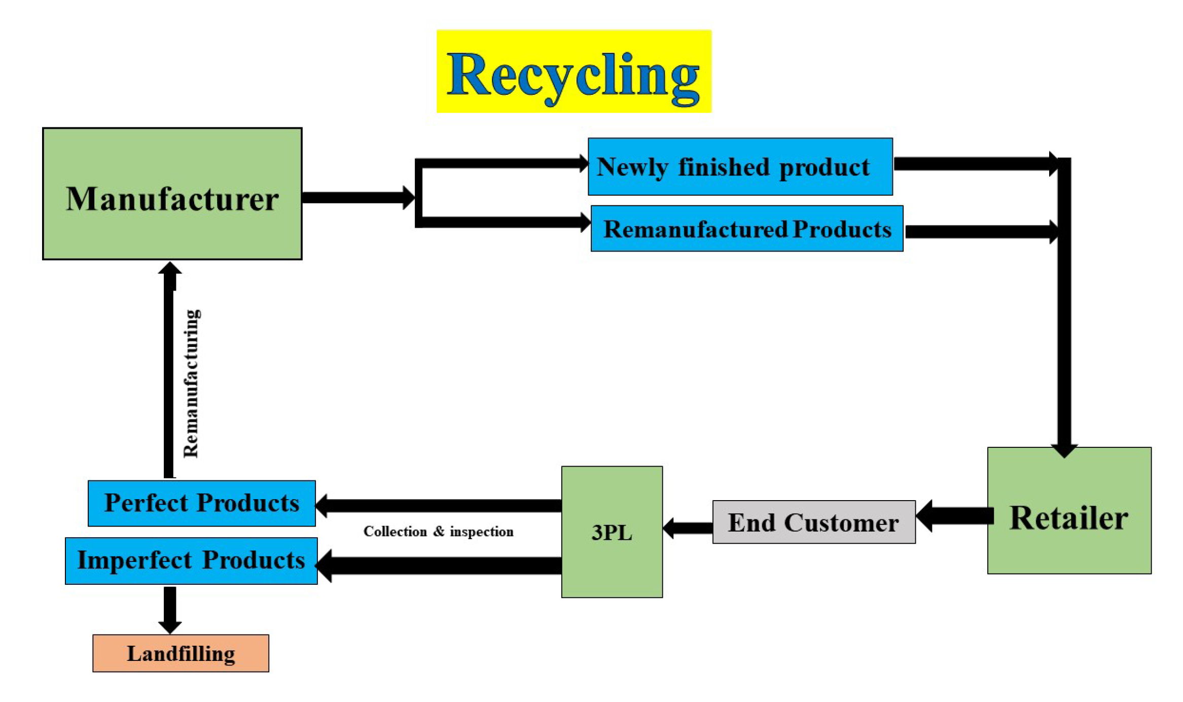
Due to short-term use of new technology, the life cycle of products decreases gradually. As a result, the amount of EOL waste is increased which results in environmental pollution and damages human health. Therefore, recycling the waste through collection, inspection, remanufacturing, landfill, and reusing besides manufacturing newish products is the ultimate goal of this paper. A CLSCM is apprised here in which manufacturing and remanufacturing occur at the same stage and SSMD strategy is considered by the players to reduce their holding cost. Also, variable and fixed shipments and carbon emission for the manufacturer and the 3PL are envisaged for this model. The retailer uses a CAPT strategy to control carbon emissions. The 3PL is responsible for all activities such as collection, inspection, landfill, and deliveries of product to the manufacturer for remanufacturing. Then, the cycle is repeated. The whole scenario is depicted in Figure 1.

3.2. Notation

The notations are elaborately discussed in Table 2.

3.3. Assumptions

The following assumptions are made for designing the model.
  • All players of the CLSCM are in a cooperation and the power of each player is the same. No game strategy is considered for the symmetric power of the SC players. This study elaborates on a coordination policy for the cost minimization. The demand and production rates are deterministic with D < P . Thus, shortage is not allowed for this model.
  • Constant and variable shipment carbon emission costs are introduced for the SSMD policy. This study adopts the variable shipment and carbon emission costs depending on the container quantity and distance between players.
  • To help alleviate global warming due to carbon emissions, a CAPT strategy is considered by the retailer for a definite period in which it can sell or buy carbon credit regarding its own carbon emissions quantity to help control carbon emission (Hua et al. [32]).
  • Two kinds of goods (newish from raw materials and remanufactured from collected used goods) are produced. The retailer and end customer bare a similar cost for both. It is further assumed that the manufacturing cost is larger than the remanufacturing cost, which is larger than the raw material price for remanufacturing used products, i.e., B m R < B m B < C m P .
  • A fraction ρ of the total demand D is collected by 3PL as recyclable goods, and it is obtained that ξ is the fraction of collected products that are defective after inspection, which are fully used for landfill, where 0 < ξ < 1 . A two-stage inspection policy is performed by 3PL before the delivery of products to the manufacturer. At the time of inspection, inspectors may wrongly reject a faultless product as faulty, which is defined as a Type I error, and may wrongly accept a faulty product as faultless, which is defined as a Type II error (Sarkar and Saren [38]). Hence, two kinds of inspection errors may occur during human inspection.
  • The manufacturer’s manufacturing/remanufacturing capacity is unlimited and both remanufactured and newly finished products have the same quality and price. The players use same type container for the delivery of products (Sarkar et al. [16]). The container number is considered as an integer. Collection, shipping, inspection, and delivery of the used products to the manufacturer are all the responsibility of 3PL. It is assumed that the random variables ρ , ξ , r 1 , r 2 are mutually independent and each pursues the same distribution (uniform) in this model.

4. Model Formulation

The retailer’s order size is Q while the manufacturer’s production volume at a single stage is s m Q . The finished products and used products are transferred between players in same-sized separate batches through a SSMD policy. Thus, a fixed and variable shipment cost is considered here. A carbon cap policy is adopted by the retailer for controlling carbon emissions due to replenishment order and inventory. After collecting used goods from the customers, the 3PL inspects the used goods and separates the defective items for landfill. In this model, the 3PL offers price discounts for each product such that the manufacturer accepts used products from the 3PL, even though the manufacturer bares the raw material price for remanufacturing each item. On this basis, this paper generates a mathematical diagram on recycling to reach the main goal of the CLSCM (see Figure 2).

4.1. Manufacturer’s Model

The manufacturer has an infrastructure for producing s m Q products, where the retailer’s order size is Q. The manufacturer has to pay holding costs for both newly finished products and collected used products. The manufacturer uses the SSMD policy for product delivery to the retailer. Therefore, the number of shipments increases, causing carbon emissions to increase. Besides the fixed shipment, and carbon emission costs, variable shipment, and carbon emission costs are also introduced. Manufacturing, remanufacturing, and buying raw materials for production are all the responsibility of the manufacturer. All cost components relative to manufacturer are discussed below.

4.1.1. Manufacturer’s Ordering Cost ( O C m )

Within a certain time period, the manufacturer orders raw materials for manufacturing new products and remanufacturing collected used products, with an ordering cost of
O C m = O s .

4.1.2. Setup Cost of the Manufacturer ( S C m )

The manufacturer produces s m Q finished goods in each production cycle. Thus, the setup cost of manufacturer is
S C m = A s .

4.1.3. Manufacturer’s Holding Cost ( H C m )

The costs to hold finished products and collected used products are not the same and therefore they are evaluated separately.

Manufacturer’s Holding Cost for Newly Made Products ( H C N m )

The manufacturer produces s m Q quantity and delivers Q quantity per shipment to the retailer through s m shipments using the SSMD policy during production. Thus, the average inventory of the manufacturer is (Kim and Sarkar [39]).
I n v A v g ( f i n i s h e d ) = s m Q Q P + s m 1 Q D s m 2 Q 2 2 P Q 2 D 1 + 2 + + ( s m 1 ) = s m Q 2 P s m 2 Q 2 2 P + s m ( s m 1 ) Q 2 2 D .
Therefore, the manufacturer’s holding expense for newly manufactured products is
H C N m = s m Q 2 P s m 2 Q 2 2 P + s m ( s m 1 ) Q 2 2 D h s .

Manufacturer’s Holding Cost for Collected Used Products ( H C R m )

As a large amount of finished goods are manufactured from EOL goods, the manufacturer has to maintain an EOL product inventory, and thus the cost function must include the manufacturer’s holding cost for collected used goods. The average stock of the manufacturer for collected used goods (Sarkar et al. [16]) is
I n v A v g ( u s e d ) = E [ ρ ] D ( 1 E [ ξ ] ) T l s m Q P + E [ ρ ] D ( 1 E [ ξ ] ) s m Q 2 P = E [ ρ ] D ( 1 E [ ξ ] ) T l s m Q 2 P .
Therefore, the manufacturer’s holding expense for collected used goods is
H C R m = E [ ρ ] D ( 1 E [ ξ ] ) T l s m Q 2 P H s .
Finally, the manufacturer’s holding cost in total is
H C m = H C N m + H C R m = s m Q 2 P s m 2 Q 2 2 P + s m ( s m 1 ) Q 2 2 D h s + E [ ρ ] D ( 1 E [ ξ ] ) T l s m Q 2 P H s .

4.1.4. Shipment Cost of the Manufacturer ( S H C m )

When the finished products are transported via manufacturer to the retailer, the manufacturer has a shipment cost. As all products (manufactured/remanufactured) are produced through a single stage and are supplied to retailer through s m lots, the fixed shipment cost is s m F . As both the quantity of containers and the distance between the manufacturer and retailer may vary, a variable shipping cost is added as C t l m r s m Q β . Thus, the total shipping cost of the manufacture is
S H C m = s m F + C t l m r s m Q β .

4.1.5. Carbon Emission Cost ( C E C m )

Due to the increasing number of shipments, the amount of carbon emissions increases. Thus, two kinds of carbon emission costs (fixed plus variable) are adopted in this model. The fixed carbon emission cost is given by C f c s s m . As carbon emissions depend upon the quantity of containers and the distance between the manufacturer and retailer, the variable carbon emission cost is given by C v c s l m r s m Q β . Thus, the total carbon emission cost is
C E C m = C f c s s m + C v c s l m r s m Q β .

4.1.6. Manufacturing Cost of the Manufacturer ( M C m )

The manufacturer produces s m Q E [ ρ ] D ( 1 E [ ξ ] ) products from new raw materials at a rate of C m P per unit. Therefore, the manufacturer’s manufacturing cost is
M C m = C m P s m Q E [ ρ ] D ( 1 E [ ξ ] ) .

4.1.7. Remanufacturing Cost of the Manufacturer ( R C m )

The manufacturer remanufactures E [ ρ ] D ( 1 E [ ξ ] ) products at an expense of B m B per unit, on that account, the remanufacturing cost of the manufacturer is
R C m = E [ ρ ] D ( 1 E [ ξ ] ) B m B .

4.1.8. Raw Material Price for Remanufacturing ( R P m )

A third party gives a price discount of d c T for each used product during delivery to the manufacturer, thus the total recycling fee is given by
R P m = E [ ρ ] D ( 1 E [ ξ ] ) B m R d c T .

4.1.9. Buying Price for Raw Materials at the Manufacturer ( B P m )

The buying price of raw materials for each unit is B m P . Therefore, the total buying price of raw material is given by
B P m = [ s m Q E [ ρ ] D ( 1 E [ ξ ] ) ] B m P .

4.1.10. Manufacturer’s Total Cost per Production Run ( T C m )

The total cost related to manufacturer is achieved by adding all costs relative to the manufacturer per cycle. On that account, the expected cost in total of the manufacturer per cycle is
T C m s m , β , T l = 1 T l [ O C m + S C m + H C m + S H C m + C E C m + M m C + R C m + R P m + B P m ] = A s + O s T l + h s D 2 T 1 P s m 1 2 P + 1 2 D 1 1 s m + H s E [ ρ ] D ( 1 E [ ξ ] ) l D 2 P + 1 T l [ s m F + C f c s s m + E [ ρ ] D 1 E [ ξ ] B m R d c T B m P + B m B C m P ] + C t l m r D β + C v c s l m r D β + D ( C m P + B m P ) .

4.2. Retailer’s Model

The retailer orders Q quantity from the manufacturer with an ordering expense of O r . The retailer pays a holding cost for finished products, buys finished products for a given price, and bares a carbon emission cost depending on the replenishment order, and a carbon emission cost related to the inventory of the retailer. A CAPT strategy is considered by the retailer to allay the volume of carbon emissions in which they can buy, sell, or transfer extra emission credit. All costs relative to retailer are described.

4.2.1. Retailer’s Ordering Cost ( O C r )

During the cycle time T l , the retailer orders for Q finished products and pays an ordering cost of O r for each order. Therefore, the ordering cost conferred by the retailer is given by
O C r = O r .

4.2.2. Retailer’s Holding Cost ( H C r )

During the period T l , the retailer receives Q products. The retailer’s holding cost for finished products is given by (Kim and Sarkar [39])
H C r = Q T l H m R 2 .

4.2.3. Buying Price of Finished Products of the Retailer ( B P r )

As the retailer pays the same amount for new/remanufactured products therefore, the total buying price paid by retailer for new/remanufactured products is given by
B P r = Q B m S .

4.2.4. Carbon Emission Cost Linked to the Replenishment Order ( C E R r )

As e unit is the amount of carbon emissions linked to the replenishment order, the carbon emission costs of the retailer related to the replenishment order is given by
C E R r = e c .

4.2.5. Carbon Emission Cost due to the Inventory of the Retailer ( C E I r )

As w unit is the amount carbon emission cost due to the inventory at retailer, hence, the average stock of the retailer is Q T l 2 , and the carbon emission costs relative to the retailer for this stock is given by
C E I r = T l Q w c 2 .

4.2.6. Total Cost Related to Retailer ( T C r )

The retailer’s aggregate cost is obtained by adding all costs related to the retailer. Consequently, the retailer’s aggregate cost is given by (see for reference Hua et al. [32]).
T C r = 1 T l [ O C r + H C r + B P r c X ] = 1 T l O r + Q T l H m R 2 + Q B m S c X ,
subject to, C E R r + C E I r + c X = c δ , i.e.,
c T l Q w 2 + e + X = c δ ,
where Equation (21) is the balance constraint of carbon, δ is the carbon emission quota, c is the carbon price per unit, and X is considered to be the excess carbon credit at retailer which he sells to another company or industry. Thus, the retailer’s per cycle expected total cost is
T C r T l = O r + Q T l H m R 2 + Q B m S + c T l Q w 2 + e δ T l = O r + c e T l + D T l ( H m R + c w ) 2 c δ T l + D B m S .

4.3. 3PL’s Model ( T C l )

After collecting used items from the customers, the 3PL inspects them to detect any defective items. Then, the 3PL delivers the perfect items to the manufacturer for remanufacturing with a discount price and uses the defective products for landfill. The manufacturer pays a raw material price for these perfect items for remanufacturing. All costs relative to 3PL are described as follows:

4.3.1. 3PL’s Collection Cost ( C T c )

The 3PL collects EOL goods from the end consumer. The collection cost of 3PL for each unit is C l C . Therefore, the total collection cost is given by
C T c = E [ ρ ] D C l C .

4.3.2. Setup Cost of 3PL ( S C l )

The setup cost for setting up the infrastructure for collecting used products is given by
S C l = C s T .

4.3.3. 3PL’s Holding Cost ( H C s )

The 3PL collects E [ ρ ] D used items and stocks them until the manufacturer asks for a delivery. The 3PL’s inventory increases gradually during this period. These products are delivered to the manufacturer after inspection. On that account, 3PL’s holding cost to hold the used products during this period is given by
H C s = E [ ρ ] D H l C T l 2 .

4.3.4. Inspection Cost ( I C l )

The 3PL applies a two-stage inspection policy to detect faulty goods and prevent the shipment of faulty goods. In this model, 3PL first applies a product inspection policy and then applies a container inspection policy for the transportation of perfect goods to the manufacturer for remanufacturing. Thus, the total inspection cost is
I C l = C c I E [ ρ ] D + C i V E [ ρ ] D ( 1 E [ ξ ] ) β .

4.3.5. Landfill Cost of 3PL ( L C l )

Please note that ξ is the fraction of collected products that are defective after inspection and hence, the number of defective items after inspection is E [ ρ ] D E [ ξ ] , which are used for landfill). Thus, the number of non-defective items after inspection is given by E [ ρ ] D ( 1 E [ ξ ] ) . As E [ ρ ] D E [ ξ ] is the quantity of products used for landfill, the total landfill cost is
L C l = E [ ρ ] D E [ ξ ] C l T .

4.3.6. Price Discounts ( P D l )

3PL offers a price discount d c T for each item to motivate the manufacturer into purchasing products. The price discount offered by 3PL to the manufacturer is given by
P D l = E [ ρ ] D ( 1 E [ ξ ] ) d c T .

4.3.7. Shipment Cost During Delivery to the Manufacturer ( S H C l )

The variable shipment cost is evaluated based on the container numbers that are used for transportation and the distance between 3PL and the manufacturer. Since 3PL ships E [ ρ ] D ( 1 E [ ξ ] ) perfect products to the manufacturer, the fixed shipment cost for delivery to the manufacturer is F s l and the variable shipment cost is C t l m l E [ ρ ] D ( 1 E [ ξ ] ) β . Therefore, the total shipping cost for the delivery of perfect products is given by
S H C l = F s l + C t l m l E [ ρ ] D ( 1 E [ ξ ] ) β .

4.3.8. Carbon Emission Cost During Dispatch to the Manufacturer ( C E C l )

Similar to previously, the fixed carbon emission cost is C f c m s l and the variable carbon emission cost is C v c m l m l E [ ρ ] D ( 1 E [ ξ ] ) β . Therefore, the carbon emission cost in total paid by the retailer during delivery to the manufacturer is given by
C E C l = C f c m s l + C v c m l m l E [ ρ ] D ( 1 E [ ξ ] ) β .

4.3.9. Inspection Error ( I E l )

At the time of inspection, inspectors may wrongly reject a faultless product as faulty, which is defined as Type I error, and may wrongly accept a faulty product as faultless, which is called a Type II error. These two kinds of inspection errors may be founded during human inspection.

Type I Error 

The number of falsely rejected faultless items is E [ ρ ] D ( 1 E [ ξ ] ) E [ r 1 ] . The total cost due to Type I errors is
E [ ρ ] D ( 1 E [ ξ ] ) E [ r 1 ] C r T .

Type II Error 

The number of falsely accepted defective items is E [ ρ ] D E [ ξ ] E [ r 2 ] . The total cost due to type II errors is
E [ ρ ] D E [ ξ ] ( 1 E [ r 2 ] ) C a T .
Hence, the total cost due to inspection errors is given by
I E l = E [ ρ ] D ( 1 E [ ξ ] ) E [ r 1 ] C r T + E [ ρ ] D E [ ξ ] ( 1 E [ r 2 ] ) C a T .

4.3.10. Total Cost of 3PL per Cycle ( T C l )

Thus, the 3PL’s expected cost in total per cycle is
T C l T l , s l , β = 1 T l C T c + S C l + H C s + I C l + L C l + P D l + S H C l + C E C l + I E l = E [ ρ ] D T l C l C + C c I + E [ ξ ] C l T + ( 1 E [ ξ ] ) d c T + ( 1 E [ ξ ] ) E [ r 1 ] C r T + E [ ξ ] ( 1 E [ r 2 ] ) C a T + 1 T l ( C i V + C t l m l + C v c m l m l ) E [ ρ ] D ( 1 E [ ξ ] ) β + E [ ρ ] D H l C 2 + C s T + s l ( F + C f c m ) T l .

4.4. Total Cost of CLSC per Cycle ( J T C )

The expected cost in total of the CLSCM is the summation of all costs corresponding to the manufacturer, retailer, and 3PL. Thus, the expected cost in total of the CLSCM per cycle is
J T C T l , s m , s l , β = T C m + T C r + T C l = A s + O s T l + h s D 2 T l 1 P s m 1 2 P + 1 2 D 1 1 s m + H s E [ ρ ] D ( 1 E [ ξ ] ) 1 D 2 P + 1 T l { s m F + C f c s s m + E [ ρ ] D 1 E [ ξ ] ( B m R d c T B m P + B m B C m P ) } + C t l m r D β + C v c s l m r D β + D ( C m P + B m P ) + O r + c e T l + D T l ( H m R + c w ) 2 c δ T l + D B m S + E [ ρ ] D T l [ C l C + C c I + E [ ξ ] C l T + ( 1 E [ ξ ] ) d c T + ( 1 E [ ξ ] ) E [ r 1 ] C r T + E [ ξ ] ( 1 E [ r 2 ] ) C a T ] + 1 T l ( C i V + C t l m l + C v c m l m l ) E [ ρ ] D ( 1 E [ ξ ] ) β + E [ ρ ] D H l C 2 + C s T + s l ( F + C f c m ) T l .

4.5. Solution Methodology

The most important decisions in this model are the optimum shipment numbers for delivery of finished goods to the retailer and used products to the manufacturer to control the waste reduction by the minimum cost. The manufacturer’s inventory relies on the quantity of finished goods that have been transported to the retailer. Generally, the retailer’s order quantity should be replenished quickly to alleviate any residual stock by the manufacturer. The retailer’s inventory plays a significant role in this model by reducing the manufacturer’s inventory holding cost. For shortened lead time, the retailer should receive the delivery quickly. Therefore, the manufacturer and the 3PL designate shipment numbers before assigning the value of the other variables. Thus, the optimal value of the replenishment cycle length T l is acquired by considering the partial derivatives of Equation (33) in regard to T l .
Rearranging the terms of Equation (33), it is found as
J T C T l , s m , s l , β = 1 T l [ A s + O s + s m F + C f c s s m + E [ ρ ] D ( 1 E [ ξ ] ) ( B m R d c T B m P + B m B C m P ) + O r + c e δ + { E [ ρ ] D C l C + H l R + C c I + E [ ξ ] C l T + ( 1 E [ ξ ] ) d c T + ( 1 E [ ξ ] ) E [ r 1 ] C r T + E [ ξ ] ( 1 E [ r 2 ] ) C a T } + ( C i V + C t l m l + C v c m l m l ) E [ ρ ] D ( 1 E [ ξ ] ) β + C s T + s l ( F + C f c m ) ] + T l h s D 2 1 P s m + 1 2 D 1 1 s m 1 2 P + D H m R + c w 2 + H s E [ ρ ] D ( 1 E [ ξ ] ) ( 1 D 2 P ) + C t l m r D β + C v c s l m r D β + D C m P + B m P + D B m S + E [ ρ ] D H l C 2 = 1 T l f 1 s m , s l , β + T l f 2 s m + f 3 β .
[See Appendix A for the values of f 1 , f 2 , f 3 .]
Differentiating Equation (34) with respect to T l , one can write
J T C z r , z l , T l , s m , s l , β T l = 1 T l 2 f 1 s m , s l , β + f 2 s m .
Equating (35) to zero, it is found
T l = f 1 s m , s l , β f 2 s m .
The shipment numbers s m , s l , and capacity of single container β can be obtained from the following relations:
J T C s m 1 J T C s m J T C s m + 1 ,
J T C s l 1 J T C s l J T C s l + 1 ,
J T C β 1 J T C β J T C β + 1 .
Lemma 1.
If s m , s l , and β are constants then the aggregate cost of the CLSCM per cycle (JTC) has the global minimum at T l = f 1 s m , s l , β f 2 s m .
Proof. 
J T C T l , s m , s l , β will have a least value at ( T l ) (continuous variable) if we can show clearly that the partial derivative second order of J T C (the complete cost function) respecting to T l is positive.
The partial derivative second order of J T C (the cost function) is
2 J T C T l , s m , s l , β T l 2 = 2 T l 3 f 1 s m , s l , β ,
which is greater than zero at T l . Thus, J T C T l , s m , s l , β has the global minimum if the other three decision variables s m , s l , and β are given. □

MHGS Algorithm

The problem in this paper is an MINLP problem, which contains both continuous and discrete variables. A MHGS algorithm is proposed for solving this model.
Step 1.
Obtain shipment numbers s m and s l is found by using a linear search method. Put all parametric data and obtain the optimal value of shipment numbersand assume the manufacturer and 3PL have a clear-cut shipment numbers.
Step 2.
Capacity of single container β , cycle length T l are obtained.
Step 2.1.
Put β = 1 .
Step 2.2.
Evaluate T l from Equation (36).
Step 3.
Calculate the total cost J T C T l , s m , s l , β from Equation (33). J T C T l , s m , s l , β is an optimum solution for fixed β .
Step 4.
Put β = β + 1 and perform Step 2.2 and 3. If J T C T l , s m , s l , β J T C T l , s m , s l β 1 , reiterate Step 2 and then go to Step 3, if not go to Step 5.
Step 5.
Put J T C T l , s m , s l , β = J T C T l , s m , s l , β 1 . J T C z r , z l , T l , s m , s l , β is the global optimal solution.

5. Numerical Experiment

Managing waste and global warming prevention has become a great challenge for industries throughout the whole world. This study proposes a CLSC in which EOL products are collected at a random rate and perfect used products are remanufactured besides the production of newly finished products to recycle and reuse wastes.
Input parameters are provided in Table 3, taken from (Sarkar et al. [31]; Sarkar et al. [16]; Hua et al. [32]; Sarkar and Saren [38]) to validate the model. Expected value of random variables are described in Appendix B. Table 4 presents the output data set relative to the input data set.
From Table 4, the optimal values for T l , s m , s l , and β are obtained. Subsequently, the corresponding values of J T C and X are determined by putting the optimal results of the corresponding decision variables in Equations (33) and (21), respectively.
The replenishment cycle length T l = 0.25 years, the shipment number for transporting newly made products to the retailer by manufacturer is s m = 4, the shipment number for transporting the collected used products by 3PL to the manufacturer is s l = 3, and the container capacity β is 4 units. From Equations (33) and (21), the optimal value are in Table 4.
The expected cost in total is J T C ( T l , s m , s l , β ) = $ 73,021 per cycle and the transfer quantum of carbon emission X = 5,089.44 unit. The most important scenario overlooked in this section is that the maximum recycling is done for these optimum values of decision variables.

5.1. Special Case 1: Model without a CAPT Strategy for the Retailer

The effect of the CAPT strategy is studied in a special case. Without a CAPT strategy, the carbon emission quota δ becomes zero and the optimal outcomes of the corresponding decision variables are shown in Table 5, given as T l = 0.96, s m = 2, s l = 2, β = 4. The cost of the CLSCM then becomes $73,375.7 per cycle. In this scenario, the outcome of the dependent variable X equals 0 unit. Thus, without a CAPT strategy, the management cost increases and hence the players of the CLSCM model are advised to consider various important costs to lessen the system’s total cost. In that case, the capacity of each container remains unaltered, which is realistic and thus validates the model. The most important scenario observed in this model is that without CAPT strategy this model converges to Sarkar et al. [16] in which the total cost per cycle was $495,874 and used products were collected at a rate of 0.423. But in this model used products are collected at a rate of 0.84 (i.e., recycling/reusing occurred at maximum level). Thus, one can easily accept this proposed approach to manage waste and reduce the total cost.

5.2. Special Case 2: Model without Reverse Logistics

This case clarifies the status of the model after neglecting the RL operation and in this situation, the model involves the costs related to the forward supply chain. The model is transformed to a function of three variables ( s m , T l , β ). Table 5 displays the optimal outcomes of the corresponding decision variables as ( s m = 2 , T l = 0.84 , β = 4 , and the total cost for the CLSCM = $73,328.9 per cycle). The result indicates that after ignoring the RL operation, the cycle time of the manufacturer T l changes to 0.84 years and the total cost changes to $73,328.9 per cycle. Thus, without RL operation, the system’s total cost increases, which can inspire industry to recycle products instead of manufacturing of newly finished products as the industry can produce the same amount of products at minimum cost and manage the waste. The capacity of each container remains unaltered, which is realistic and signifies validation of the model. Again, it is notable that without reverse logistics, this paper is similar to Sarkar et al. [31].

5.3. Special Case 3: Model without Variable Transportation and Carbon Emission

This case demonstrates the status of the model after neglecting variable transportation and carbon emission cost. In this circumstance, the optimal outcomes of the corresponding decision variables are shown in Table 5, given as T l = 0.69, s m = 4, s l = 3, and β = 4. The cost of the CLSCM then becomes $72,629 per cycle. Thus, without variable transportation and carbon emission, the system’s cost decreases but as the distances between players are not always same, the advice to the management is to consider these important costs for reality.
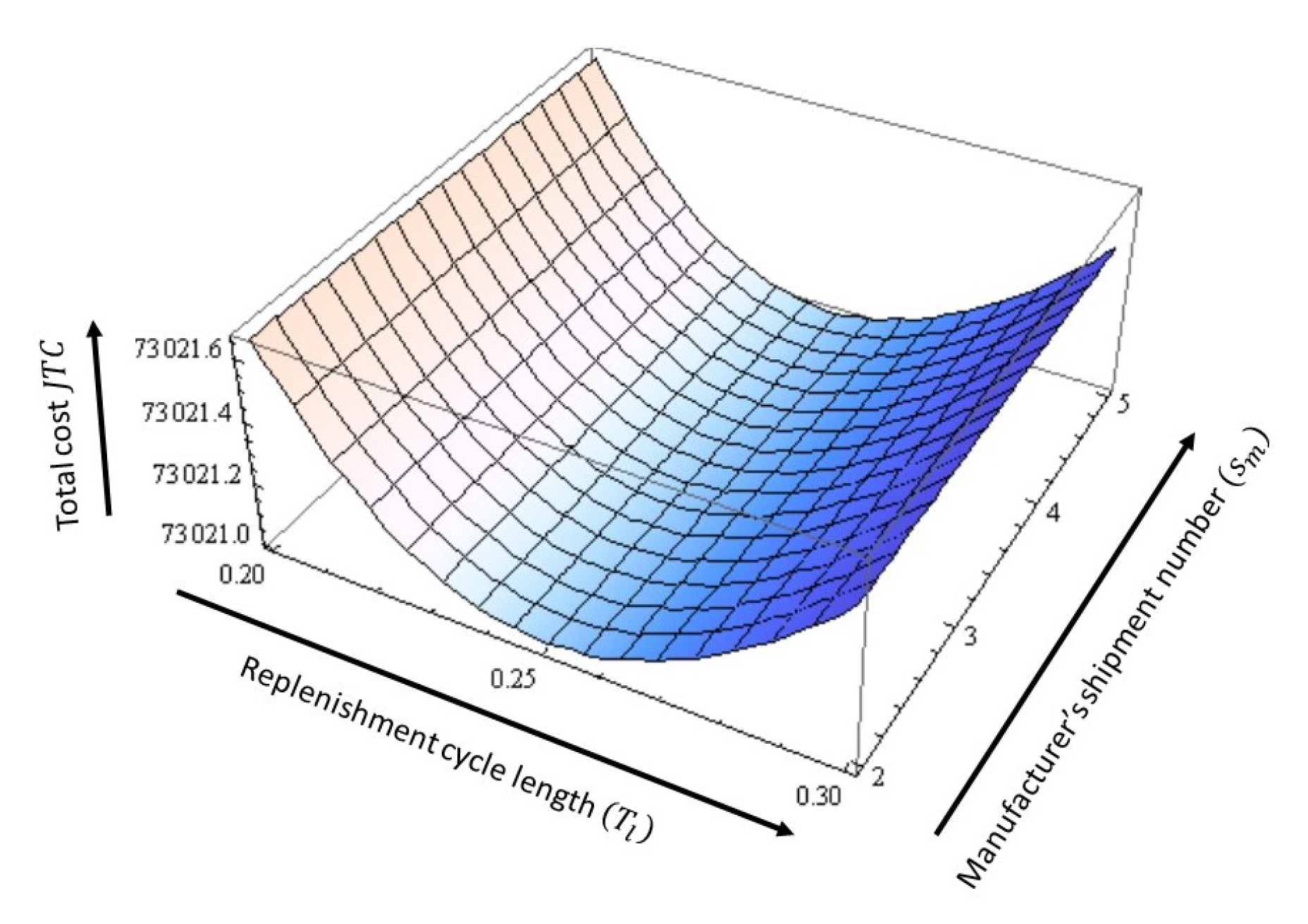
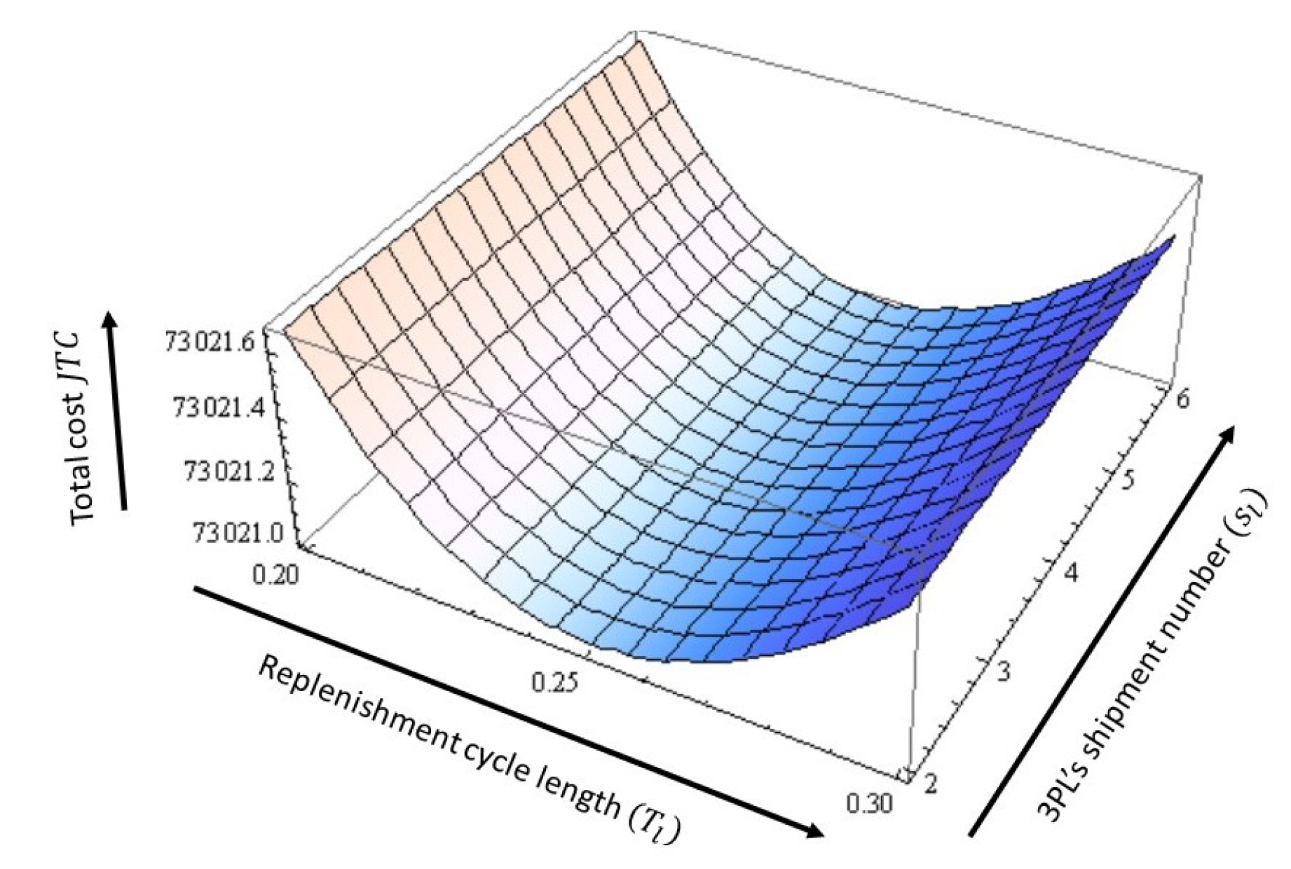
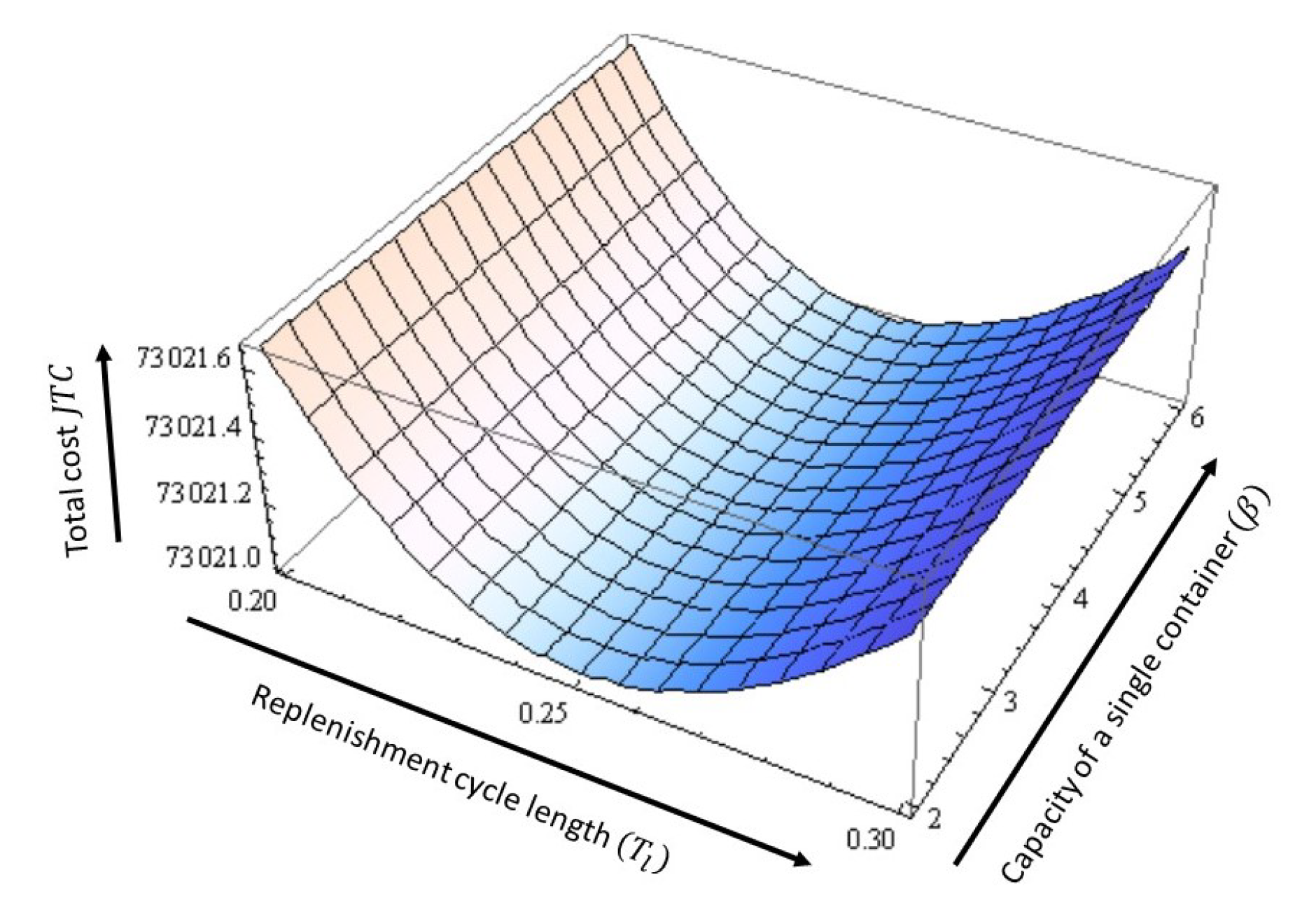
From Figure 3, Figure 4 and Figure 5 one can easily find that the graphs are convex which proves that the total cost is globally minimized.

6. Sensitivity Analysis

The sensitivity analysis in total cost for the CLSCM model with reference to each input data is conferred in Table 6.
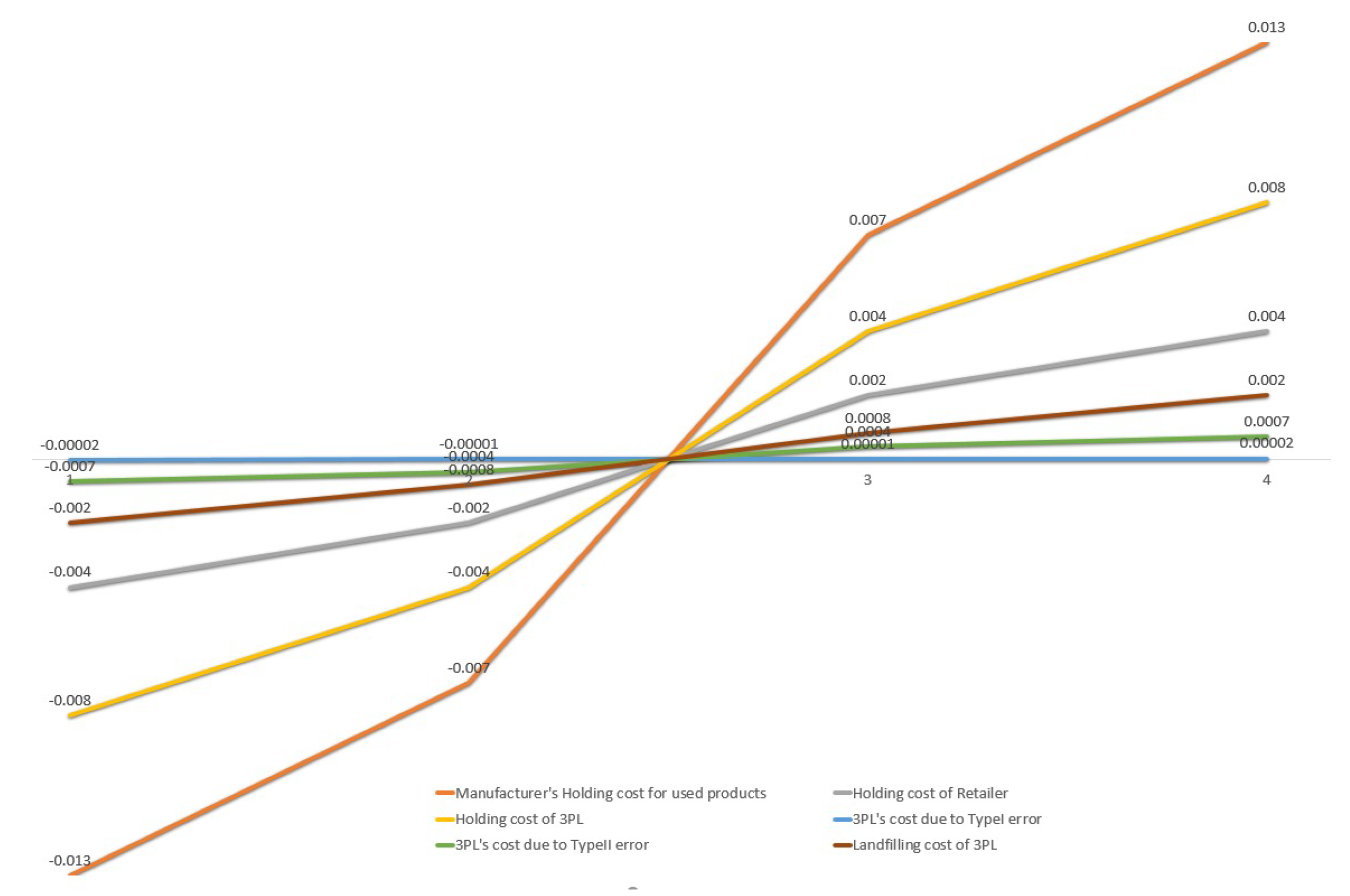
  • If the setup cost A s of the manufacturer for setting up the production infrastructure, ordering costs O s , O r relating to manufacturer and retailer, setup cost C s T per setup, and the collection cost C l C of 3PL are all increased, the total cost increases in that situation. Due to the reductions in the setup cost, ordering cost, and collection cost by 25% or 50%, infeasible results are obtained. These parameters moderately affect the models.
  • The manufacturer’s holding costs h s , H s for newly finished products and collected used products, retailer’s and 3PL’s holding costs H m R and H l C are not sensitive in this study. For negative as well as positive percent changes of the holding cost, the results are similar in magnitude to the total cost. Thus, for both changes, an equilibrium situation is observed in both directions.
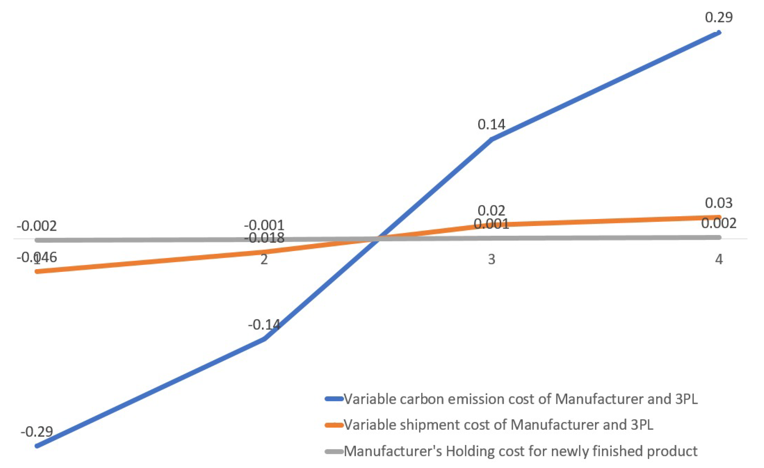
  • If the fixed shipment cost of the CLSCM model per shipment F and fixed carbon emission costs C f c s and C f c m per shipment for manufacturer and 3PL are increased by 50% and 25%, respectively, then the expected total cost increases. For decreases of C f c s and C f c m by 50% and F by 25% or more, infeasible results are obtained. Therefore, it can be concluded that these parameters moderately affect the system. Again, The expected total cost increases or decreases according as the shipment cost C t per container per unit distance increases or decreases.
  • If the carbon emission cost C v c s and C v c m per container per unit distance are increased/decreased, then the expected total cost for the CLSCM model increases/decreases, respectively. The total cost maintains a position of equilibrium and these parameters moderately affect the system.
  • It is observed that for percentage increases in the manufacturer’s production cost C m P and buying price of raw materials of the manufacturer B m P , the changes in total cost is infeasible. If the production cost and buying price of raw materials decreases by 25% or 50%, the total cost decreases. Thus, these parameters are more sensitive.
  • If the raw material’s price B m R for remanufacturing and the remanufacturing cost of the manufacturer B m B increase, then the total cost increases. Decreasing these parameters by 25% or 50% leads to infeasible results. Thus, these are sensitive parameters. Again, if the carbon price c of the retailer decreases, then the total cost increases which is a fully different scenario compared to previous parameters. But due to the increment of this parameter by 25% or 50%, an infeasible result is obtained. If less carbon cost is needed, it is very simple for any CLSC to offset total cost.
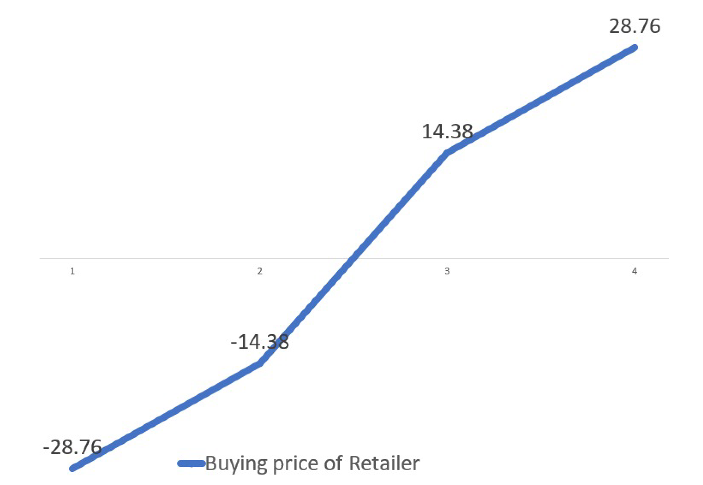
  • The buying price B m S is the most significant and sensitive parameter for this model. This model considers newly finished and finished products both. Therefore, this cost is very effective and it is clear from sensitivity analysis that if the buying price of finished product B m S of retailer decreases by 50%, then the optimal cost decreases by 28.76%.
  • The total cost of CLSCM is increased if per-unit inspection cost C c I is increased. Here, it is noticed that if the parameter C c I is decreased by 25% or more, an infeasible result is obtained. Again, if the variable inspection cost C i V per container increases, then the expected total cost increases. If the parameters C i V decreases by 25% or more, an infeasible result is obtained. Therefore, it is not possible to decrease the inspection cost by 25% or more.
  • The landfill cost C l T , price discounts d c T , cost of wrongly rejecting good items C r T , and cost of wrongly accepting faulty items C a T are the least sensitive parameters in this model. For positive/negative change of each parameter, an equilibrium situation is arrived.
Graphically, the effect of changes in total cost for changes of different parameters are illustrated in Figure 6, Figure 7 and Figure 8.

7. Implications and Managerial Insights

To recycle the waste and minimize the cost of this CLSCM under a CAPT mechanism, it is very important to verify the total system from all view points.
To increase the lifecycle of each product, the management begins remanufacturing used products after inspecting them. The SSMD policy is introduced here, for which the amount of carbon emission increases. the management has to decide how the carbon emission cost can be reduced, which can be a very difficult situation. This problem is solved by the proposed model.
  • From sensitive analysis, it is evident that if the carbon price of the retailer decreases, the total cost is increased. This is because the retailer uses a CAPT mechanism (in which they can sell the extra carbon credit).
  • It is observed that if the buying cost of newish/remanufactured products is at a minimum, the total cost is at a minimum. Therefore, industry managers can easily make decisions considering these findings. Here, each of the random variables (like return rate of used goods, defective rate of collected used products and also the random variables presenting Type I and Type II errors) follow the uniform distributions, from which the global minimum expense can be calculate by the industry easily.

8. Conclusions

This paper proposed a three-layer CLSCM where the manufacturer was reliable. The ultimate goal of this model was to optimize the aggregate cost through recycling and reusing of waste. Besides fixed shipment and carbon emission costs, this model considered variable shipment and carbon emission costs relying on the number of containers and distance. When using the SSMD policy, the carbon emission cost increased. For this, a carbon CAPT strategy was considered for the retailer in this model. A model (MINLP) and a corresponding algorithm was designed to solve, and the total system cost was minimized along with the replenishment cycle length, shipment numbers, and capacity of each container. Finally, the total cost was minimized. However, what will be the situation if any player in the SCM faces damage due to the coordination policy? What will be the procedure of the compensate policy? This situation can be studied in a future extension of this study. Apart from the symmetric power of coordination, the situation for the asymmetric power for the SC players can be considered for the future extension of the study. Since the used products are collected at a random rate, uncertainty appears in the SC because of uncertain returns, finally leading to uncertain production. Thus, this work can be extended by proposing a variable production rate. A multi-stage production system can also be considered to avoid waste. In this situation, the expected cost in total can be reduced by introducing a discrete setup cost, which can reduce the total cost. For collecting EOL goods, the 3PL can make an elementary investment into the collection centrum. To diminish the environmental impact and enhance resource use, one can also consider a multi-retailer setup for future work. For future investigations, it can be assumed that product delivery is performed offline, whereas orders can be done online. In this case, the demand will become advertisement-dependent. The random variables could also follow Beta, Triangular, or Double Triangular distributions. Finally, this model can be elongated by considering product delivery via drones (i.e., not using human beings).

Author Contributions

Conceptualization, writing review, B.S.; Methodology, M.M.; Software, M.M.; Validation, B.S., S.K.G. and M.M.; Data curation, B.S.; Writing—Original draft preparation, M.M., writing–review and editing, S.K.H. All authors have read and agreed to the published version of the manuscript.

Funding

There is no funding for the research.

Conflicts of Interest

The authors declare no conflict of interest.

Abbreviations

The following abbreviations are used in this manuscript:
SSCsustainable supply chain
EOLend-of-life
CLSCMclosed-loop supply chain management
SSMDsingle-setup multi-delivery
SCsupply chain
SCMsupply chain management
CAPTcap-and-trade
GSCMgreen supply chain management
RLreverse logistics
RLSCreverse logistics supply chain
VMIPvendor-managed-inventory policy
3PLthird party logistics

Appendix A

f 1 s m , s l , β = [ A s + O s + s m F + C f c s s m + E [ ρ ] D ( 1 E [ ξ ] ) ( B m R d c T B m P + B m B C m P ) + O r + c e δ + E [ ρ ] D C l C + H l R + C c I + E [ ξ ] C l T + ( 1 E [ ξ ] ) d c T + ( 1 E [ ξ ] ) E [ r 1 ] C r T + E [ ξ ] ( 1 E [ r 2 ] ) C a T + ( C i V + C t l m l + C v c m l m l ) E [ ρ ] D ( 1 E [ ξ ] ) β + C s T + s l ( F + C f c m ) ] , f 2 s m = h s D 2 1 P s m + 1 2 D 1 1 s m 1 2 P + D H m R + c w 2 , f 3 β = H s E [ ρ ] D ( 1 E [ ξ ] ) 1 D 2 P + C t l m r D β + C v c s l m r D β + D C m P + B m P + D B m S + E [ ρ ] D H l C 2 .

Appendix B

It is assumed that each of ρ , ξ , r 1 , r 2 follows uniform distribution and the probability density functions corresponding to these uniform distributions are
f ( x ) = { 1 ρ 2 ρ 1 ; ρ 1 x ρ 2 0 ; Otherwise
g ( x ) = { 1 ξ 2 ξ 1 ; ξ 1 x ξ 2 0 ; Otherwise
h ( x ) = { 1 r 12 r 11 ; r 11 x r 12 0 ; Otherwise
u ( x ) = { 1 r 22 r 21 ; r 21 x r 22 0 ; Otherwise
The expected value of ρ is
E ( ρ ) = ρ 1 ρ 2 x f ( x ) d x = ρ 1 ρ 2 x ρ 2 ρ 1 d x = ρ 2 2 ρ 1 2 2 ( ρ 2 ρ 1 ) = ρ 1 + ρ 2 2 .
Similarly, the expected values of ξ , r 1 and r 2 are
E ( ξ ) = ξ 1 + ξ 2 2 , E ( r 1 ) = r 11 + r 12 2 , E ( r 2 ) = r 21 + r 22 2 .

References

  1. Tayyab, M.; Jemai, J.; Lim, H.; Sarkar, B. A sustainable development framework for a cleaner multi-item multi-stage textile production system with a process improvement initiative. J. Clean. Prod. 2020, 246, 119055. [Google Scholar] [CrossRef]
  2. Tiwari, S.; Ahmed, W.; Sarkar, B. Sustainable ordering policies for non-instantaneous deteriorating items under carbon emission and multi-trade-credit-policies. J. Clean. Prod. 2019, 240, 118183. [Google Scholar] [CrossRef]
  3. Cárdenas-Barrón, L.E.; González-Velardeb, J.L.; Treviño-Garza, G.; Garza-Nuñeza, D. Heuristic algorithm based on reduce and optimize approach for a selective and periodic inventory routing problem in a waste vegetable oil collection environment. Int. J. Prod. Econ. 2019, 211, 44–59. [Google Scholar] [CrossRef]
  4. Cárdenas-Barrón, L.E.; Sana, S.S. A production-inventory model for a two-echelon supply chain when demand is dependent on sales teams’ initiatives. Int. J. Prod. Econ. 2014, 155, 249–258. [Google Scholar] [CrossRef]
  5. Taleizadeh, A.A.; Noori-daryan, M.; Cárdenas-Barrón, L.E. Joint optimization of price, replenishment frequency, replenishment cycle and production rate in vendor managed inventory system with deteriorating items. Int. J. Prod. Econ. 2015, 155, 285–295. [Google Scholar] [CrossRef]
  6. Hota, S.K.; Sarkar, B.; Ghosh, S.K. Effects of unequal lot size and variable transportation in unreliable supply chain management. Mathematics 2020, 8, 357. [Google Scholar] [CrossRef] [Green Version]
  7. Daryanto, Y.; Wee, H.M.; Widyadana, G.A. Low carbon supply chain coordination for imperfect quality deteriorating items. Mathematics 2019, 7, 234. [Google Scholar] [CrossRef] [Green Version]
  8. Mishra, U.; Wu, J.Z.; Sarkar, B. A sustainable production-inventory model for a controllable carbon emissions rate under shortages. J. Clean. Prod. 2020, 256, 120268. [Google Scholar] [CrossRef]
  9. Ullah, M.; Sarkar, B. Recovery-channel selection in a hybrid manufacturing-remanufacturing production model with RFID and product quality. Int. J. Prod. Econ. 2020, 219, 360–374. [Google Scholar] [CrossRef]
  10. Taleizadeh, A.A.; Soleymanfar, V.R.; Govindan, K. Sustainable economic production quantity models for inventory systems with shortage. J. Clean. Prod. 2018, 174, 1011–1020. [Google Scholar] [CrossRef]
  11. Ahamed, W.; Sarkar, B. Management of next-generation energy using a triple bottom line approach under a supply chain framework. Resour. Conserv. Recyc. 2019, 150, 104431. [Google Scholar] [CrossRef]
  12. Sarkar, B.; Tayyab, M.; Kim, N.; Habib, M.S. Optimal production delivery policies for supplier and manufacturer in a constrained closed-loop supply chain for returnable transport packaging through metaheuristic approach. Comp. Indus. Eng. 2019, 135, 987–1003. [Google Scholar] [CrossRef]
  13. Sarkar, B.; Majumdar, A. Integrated vendor–buyer supply chain model with vendor’s setup cost reduction. App. Math. Comp. 2013, 224, 362–371. [Google Scholar] [CrossRef]
  14. Sarkar, B. A production-inventory model with probabilistic deterioration in two-echelon supply chain management. App. Math. Mod. 2013, 37, 3138–3151. [Google Scholar] [CrossRef]
  15. Cárdenas-Barrón, L.E.; Chung, K.J.; Treviño-Garza, G. Celebrating a century of the economic order quantity model in honor of Ford Whitman Harris. Int. J. Prod. Econ. 2014, 155, 1–7. [Google Scholar] [CrossRef]
  16. Sarkar, B.; Ullah, M.; Kim, N. Environmental and economic assessment of closed-loop supply chain with remanufacturing and returnable transport items. Comp. Indus. Eng. 2017, 111, 148–163. [Google Scholar] [CrossRef]
  17. Sarkar, B.; Omair, M.; Kim, N. A cooperative advertising collaboration policy in supply chain management under uncertain conditions. Appl. Sci. Comp. 2020, 88, 105948. [Google Scholar]
  18. Cárdenas-Barrón, L.E.; Sana, S.S. Multi-item EOQ inventory model in a two-layer supply chain while demand varies with promotional effort. App. Math. Mod. 2015, 39, 6725–6737. [Google Scholar] [CrossRef]
  19. Guide, V.D.R., Jr.; Van Wassenhove, L.N. The evolution of closed-loop supply chain research. Oper. Res. 2009, 57, 10–18. [Google Scholar] [CrossRef]
  20. Saxena, N.; Sarkar, B.; Singh, S.R. Selection of remanufacturing/production cycles with an alternative market: A perspective on waste management. J. Clean. Prod. 2020, 245, 118935. [Google Scholar] [CrossRef]
  21. Govindan, K.; Soleimani, H. A review of reverse logistics and closed-loop supply chains: A Journal of Cleaner Production focus. J. Clean. Prod. 2016, 142, 371–384. [Google Scholar] [CrossRef]
  22. Govindan, K.; Soleimani, H.; Kannan, D. Reverse logistics and closed-loop supply chain: A comprehensive review to explore the future. Eur. J. Oper. Res. 2015, 240, 603–626. [Google Scholar] [CrossRef] [Green Version]
  23. Shaharudin, M.R.; Govindan, K.; Zailani, S.; Tan, K.C. Managing product returns to achieve supply chain sustainability: An exploratory study and research propositions. J. Clean. Prod. 2015, 101, 1–15. [Google Scholar] [CrossRef]
  24. Huang, X.; Choi, S.M.; Ching, W.K.; Siu, T.K.; Huang, M. On supply chain coordination for false failure returns: A quantity discount contract approach. Int. J. Prod. Econ. 2011, 133, 634–644. [Google Scholar] [CrossRef]
  25. Heydari, J.; Govindan, K.; Jafari, A. Reverse and closed loop supply chain coordination by considering government role. Trans. Res. Part D 2017, 52, 379–398. [Google Scholar] [CrossRef]
  26. Govindan, K.; Popiuc, M.N. Reverse supply chain coordination by revenue sharing contract: A case for the personal computers industry. Eur. J. Oper. Res. 2014, 233, 326–336. [Google Scholar] [CrossRef]
  27. Konstantaras, I.; Skouri, K.; Jaber, M.Y. Lot sizing for a recoverable product with inspection and sorting. Comp. Indus. Eng. 2010, 58, 452–462. [Google Scholar] [CrossRef]
  28. Khouja, M. Optimizing inventory decisions in a multi-stage multi-customer supply chain. Trans. Res. Part E Log. Trans. Rev. 2003, 39, 193–208. [Google Scholar] [CrossRef]
  29. Cárdenas-Barrón, L.E. Optimizing inventory decisions in a multi-stage multi-customer supply chain: A note. Trans. Res. Part E Log. Trans. Rev. 2007, 43, 647–654. [Google Scholar] [CrossRef]
  30. Ertogral, K.; Darwish, M.; Ben-Daya, M. Production and shipment lot sizing in a vendor-buyer supply chain with transportation cost. Eur. J. Oper. Res. 2007, 176, 1592–1606. [Google Scholar] [CrossRef]
  31. Sarkar, B.; Ganguly, B.; Sarkar, M. Effect of variable transportation and carbon emission in a three-echelon supply chain model. Trans. Res. Part E Log. Trans. Rev. 2016, 91, 112–128. [Google Scholar] [CrossRef]
  32. Hua, G.; Cheng, T.C.E.; Wang, S. Managing carbon footprints in inventory management. Int. J. Prod. Econ. 2011, 132, 178–185. [Google Scholar] [CrossRef]
  33. Shaw, B.K.; Sangal, I.; Sarkar, B. Joint effects of carbon emission, deterioration, and multi-stage inspection policy in an integrated inventory model. In Optimization and Inventory Management; Shah, N., Mittal, M., Eds.; Springer: Singapore, 2020; pp. 195–208. [Google Scholar]
  34. Tiwari, S.; Ahmed, W.; Sarkar, B. Multi-item sustainable green production system under trade-credit and partial backordering. J. Clean. Prod. 2018, 204, 82–95. [Google Scholar] [CrossRef]
  35. Ahmed, W.; Sarkar, B. Impact of carbon emissions in a sustainable supply chain management for a second generation biofuel. J. Clean. Prod. 2018, 186, 807–820. [Google Scholar] [CrossRef]
  36. Wang, Y.; Chen, W.; Liu, B. Manufacturing/remanufacturing decisions for a capital-constrained manufacturer considering carbon emission cap and trade. J. Clean. Prod. 2017, 140, 1118–1128. [Google Scholar] [CrossRef]
  37. Sarkar, B.; Saren, S.; Sinha, D.; Hur, S. Effect of unequal lot sizes, variable setup cost, and carbon emission cost in a supply chain model. Math. Prob. Eng. 2015, 469486. [Google Scholar] [CrossRef] [Green Version]
  38. Sarkar, B.; Saren, S. Product inspection policy for an imperfect production system with error and warranty cost. Eur. J. Oper. Res. 2016, 248, 263–271. [Google Scholar] [CrossRef]
  39. Kim, S.J.; Sarkar, B. Supply chain model with stochastic lead time, trade-credit financing, and transportation discounts. Mathematics 2017, 6465912. [Google Scholar] [CrossRef]
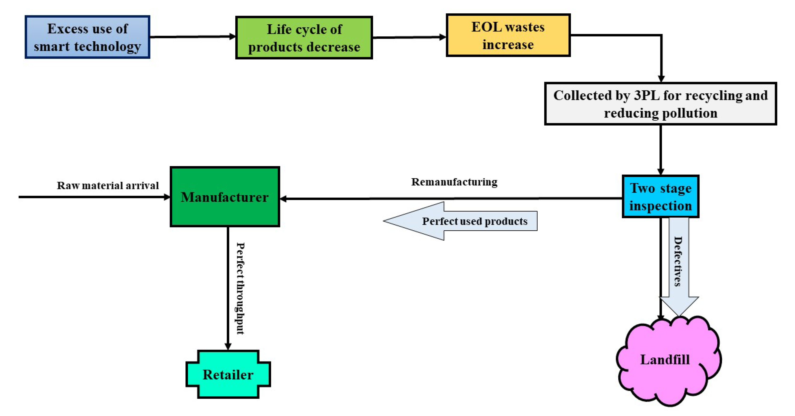
Figure 1. Problem description.
Mathematics 08 00466 g001
Figure 2. CLSCM diagram for recycling.
Mathematics 08 00466 g002
Figure 3. Total cost (JTC) for the CLSC versus manufacturer’s shipment number ( s m ) and replenishment cycle length ( T l ) when s l and β are fixed, s m and T l are variable.
Mathematics 08 00466 g003
Figure 4. Total cost (JTC) for the CLSC versus 3PL’s shipment number ( s l ) and replenishment cycle length ( T l ) when s m and β are fixed, s l and T l are variable.
Mathematics 08 00466 g004
Figure 5. Total cost (JTC) for the CLSC versus capacity of a single container ( β ) and replenishment cycle length ( T l ) when s m and s l are fixed, β and T l are variable.
Mathematics 08 00466 g005
Figure 6. Effect of changes of total cost for changes of various parameters.
Mathematics 08 00466 g006
Figure 7. Effect of changes of total cost for changes of various parameters.
Mathematics 08 00466 g007
Figure 8. Effect of change of total cost for change of buying price of retailer.
Mathematics 08 00466 g008
Table 1. Author(s) comparison Table.
Author(s)CLSCM and
SSMD
ShipmentEnvironmental
Effect
ReuseStrategy
Cárdenas-Barrón
and Sana [18]
Const.Delay
in payment
Daryanto et al. [7]SSMDVariableCE,
carbon tax
Hua et al. [32]CE,
carbon CAPT
Huang et al. [24]SSMDConst.Quantity
discount
Heydari et al. [25]CLSCMConst.Remanuf-
acturing
Price
discount
Sarkar et al. [16]CLSCM and
SSMD
VariableCERemanuf-
acturing
Taleizadeh et al. [10]CEShortage,
back-
ordering
Khouja et al. [28]SSMDConst.
Sarkar et al. [37]SSMDVariableCEReworking
This modelCLSCM and
SSMD
VariableCE,
carbon CAPT
LFPrice
discount
“—” indicates the concept does not exist for the research, Const. means constant, CE means Carbon emission, LF means landfill.
Table 2. Symbol description.
Decision Variables
T l replenishment cycle length (year)
s m shipment numbers in a cycle for delivering the finished goods to the retailer
via manufacturer (integer number)
s l shipment numbers in a cycle for delivering the used goods to the manufacturer
via 3PL (integer number)
β capacity of a single container (units)
Dependent variable
Xtransfer quantity of carbon emissions (units)
Random variables
ρ collection rate of 3PL for the used products (units/cycle)
ξ fraction of collected products that are defective due to inspection
and are used for landfill
r 1 random variable presenting Type I error
r 2 random variable presenting Type II error
Parameters
Qretailer’s ordering quantity (units)
Pproduction rate per year (units/year)
Drate of demand (units/year)
C m P manufacturer’s unit production expense ($/unit)
h s manufacturer’s holding cost to hold finished products ($/unit/unit time)
A s manufacturer’s setup expense per setup ($/setup)
O s manufacturer’s per-order ordering expense ($/order)
B m P buying price of raw material for manufacturing ($/unit)
B m B manufacturer’s remanufacturing cost ($/unit)
H s manufacturer’s holding cost to hold used goods ($/unit/unit time)
B m S buying price of new/remanufactured products of the retailer ($/unit)
H m R retailer’s holding cost to hold finished goods ($/unit)
O r retailer’s ordering cost per order ($/order)
δ carbon emission quota (units/cycle)
eunit carbon emission linked to the replenishment order (unit)
wunit variable carbon emission at the warehouse due to retailer’s inventory (unit)
ccarbon price of the retailer ($/unit)
B m R raw material price for remanufacturing paid by the manufacturer to 3PL ($/unit)
C l C collection cost of 3PL ($/unit)
C s T setup cost paid by 3PL per setup ($/setup)
H l C holding cost paid by 3PL to hold collected products ($/unit/unit time)
C c I inspection cost of 3PL ($/unit)
C i V variable inspection cost of 3PL container to deliver products to the
manufacturer ($/container)
C l T landfill cost of 3PL ($/unit)
d c T price discount offered to the manufacturer by 3PL ($/unit)
C a T cost of wrongly accepting faulty items ($/unit)
C r T cost of wrongly rejecting faultless items ($/unit)
Ffixed shipment cost of the CLSC ($/shipment)
C t shipment cost conferred by the manufacturer and 3PL per container per unit distance
($/container/km)
l m r distance of the retailer from manufacturer (kilometers)
l m l distance of the manufacturer from 3PL (kilometers)
C f c s fixed carbon emission cost paid by manufacturer per shipment for the delivery
of finished products ($/shipment)
C v c s carbon emission cost paid by manufacturer per container at unit distance for the
delivery of finished products ($/container/kilometer)
C f c m fixed carbon emission cost paid by 3PL per shipment to deliver used
products to the manufacturer ($/shipment)
C v c m carbon emission cost paid by 3PL per container per unit distance to deliver used
products to the manufacturer ($/container/kilometer)
Table 3. Input data set.
Parameters for the Manufacturer
A s = $ 200/setup O s = $ 120/order h s = $ 0.28/unit/unit time
H s = $ 0.22/unit/ unit time P = $ 452 units/year F = $ 300/shipment
C f c s = $ 2/shipment C v c s = $ 0.2/container/unit distance l m r = 60 km
B m P = $ 60/unit B m R = $ 45/unit B m B = $ 144/unit
C t = $ 0.01/container/
unit distance
C m P = $ 158/unit
Parameters for the retailer
D = $ 140 units/year O r = $ 52/order C = $ 0.2/unit
e = 720 units H m R = $ 0.32/unit/unit time w = 1.5 unit
B m s = $ 300/unit δ = 5816 units
Parameters for the 3PL
ρ 1 = 0.8 ρ 2 = 0.88 ξ 1 = 0.06
ξ 2 = 0.14 C s T = $ 35/setup C l C = $ 11.6/unit
H l C = $ 0.22/unit/unit time C c I = $ .12/unit C i V = $ 2/unit
C l T = $ .05/unit d c T = $ 1/unit C f c m = $ 2/shipment
C v c m = $ 0.2/container/
unit distance
r 11 = 0.006 l m l = 25 km
r 12 = 0.014 r 21 = 0.02 r 22 = 0.06
C r T = $ 0.01/unit C a T = $ 0.023/unit
Table 4. Optimal outcomes of the corresponding decision variables.
Decision Variables s m s l T l β JTC
Optimum Results430.25473,021
Table 5. Optimal outcomes of the corresponding decision variables under Special Cases.
Decision Variables s m s l T l β JTC
Optimal results under Special Case 1220.96473,375.7
Optimal results under Special Case 2200.84473,328.9
Optimal results under Special Case 3430.69472,629
Table 6. Sensitivity analysis of known parameters.
ParametersChanges of
Inputs (%)
Change of
JTC (%)
ParametersChanges of
Inputs (%)
Changes of
JTC (%)
A s −50N.F. C m P −50−13.3
−25N.F.−25−6.3
+25+ 0.11+25N.F.
+50+0.17+50N.F.
O s −50N.F. B m P −50−4.6
−25N.F.−25−2.1
+25+ 0.08+25N.F.
+50+0.12+50N.F.
h s −50−0.002 B m R −50N.F.
−25−0.001−25N.F.
+25+0.001+25+0.66
+50+0.002+50+.96
H s −50−0.013 B m B −50N.F.
−25−0.007−25N.F.
+25+0.007+25+1.22
+50+0.013+50+1.74
F−50N.F. O r −50N.F.
−25N.F.−25N.F.
+25+0.43+25+0.04
+50+0.62+50+0.07
C t −50−0.046c−50+0.04
−25−0.018−25+0.03
+25+0.02+25N.F.
+50+0.03+50N.F.
C f c s −50N.F. H m R −50−0.004
−25−0.01−25−0.002
+25+0.001+25+0.002
+50+0.018+50+0.004
C v c s −50−0.29 B m S −50−28.76
−25−0.14−25−14.38
+25+0.14+25+14.38
+50+0.29+50+28.76
C s T −50N.F. d c T −500.00
−25N.F.−250.00
+25+0.033+250.00
+50+0.055+500.00
C l C −50N.F. C f c m −50N.F.
−25N.F.−25−0.01
+25+ 0.334+25+0.01
+50+ 0.495+50+0.02
H l C −50−0.008 C v c m −50−0.29
−25−0.004−25−0.14
+25+0.004+25+0.14
+50+0.008+50+0.29
C c I −50N.F. C r T −50−0.00002
−25N.F.−25−0.00001
+25+0.02+25+0.00001
+50+0.03+50+0.00002
C l T −50−0.002 C a T −50−0.0007
−25−0.0008−25−0.0004
+25+0.0008+25+0.0004
+50+0.002+50+0.0007
C i V −50N.F
−25N.F.
+25+0.05
+50+0.07
N.F. means not feasible.