Mathematical Models for Stress–Strain Behavior of Nano Magnesia-Cement-Reinforced Seashore Soft Soil

Abstract

The stress–strain behavior of nano magnesia-cement-reinforced seashore soft soil (Nmcs) under different circumstances exhibits various characteristics, e.g., strain-hardening behavior, falling behavior, S-type falling behavior, and strong softening behavior. This study therefore proposes a REP (reinforced exponential and power function)-based mathematical model to simulate the various stress–strain behaviors of Nmcs under varying conditions. Firstly, the mathematical characteristics of different constitutive behaviors of Nmcs are explicitly discussed. Secondly, the conventional mathematical models and their applicability for modeling stress–strain behavior of cemented soil are examined. Based on the mathematical characteristics of different stress–strain curves and the features of different conventional models, a simple mathematical REP model for simulating the hardening behavior, modified falling behavior and strong softening behavior is proposed. Moreover, a CEL (coupled exponential and linear) model improved from the REP model is also put forth for simulating the S-type stress–strain behavior of Nmcs. Comparisons between conventional models and the proposed REP-based models are made which verify the feasibility of the proposed models. The proposed REP-based models may facilitate researchers in the assessment and estimation of stress–strain constitutive behaviors of Nmcs subjected to different scenarios.

1. Introduction

Soft soil is widely distributed in coastal areas with many defects such as large natural moisture content, excessive compression capacity, and poor bearing capacity [1,2,3]. In geotechnical engineering, deep mixing method is generally adopted to improve the strength of soil by adding cement to the soil [4,5,6,7,8]. The soft soil is reinforced to impart higher strength through a series of reactions between raw materials and curing agent [9,10,11,12,13,14,15,16]. In addition to the traditional cement curing agent, researchers are constantly looking for some novel materials such as nano materials to improve the bearing capacity of the soft soil layer [2,3,14,15,17,18,19,20].

Nano cemented soil refers to the cement-soil mixture which is improved by adding nano materials as admixtures into the mixture of water, cement and soil [20,21,22]. At present, the nano materials for enhancing cemented soil mainly include nano titanium oxide, nano montmorillonite, nano magnesia, nano silicon, nano alumina, etc. Previous experimental results show that adding nano admixtures can improve the performances of cemented soil such as its soil strength and anticorrosive properties. Based on some recent studies [2,3], nanometer magnesia (Nm) can be added into cemented soil to improve its mechanical performance.

In the past few years, mathematical models have been adopted to study the stress–strain response of soils [23,24,25,26,27,28,29,30,31]. In term of the stress–strain behaviors of cemented soil, a large number of researches have been reported [2,3,5,6,13,14,15,16,17,18,32,33,34,35,36,37]. However, the reported mathematical models have some limitations particularly in the modeling of the constitutive behavior of nano magnesia-cement-reinforced seashore soft soil (Nmcs) which manifests different stress–strain behaviors under varying conditions [2,3,4,17,18,38,39].

This study aims to propose a REP (reinforced exponential and power function)-based mathematical model to simulate the various stress–strain behaviors of Nmcs under varying circumstances. The mathematical characteristics of different constitutive behaviors are firstly examined. Then, the conventional mathematical models for stress–strain behavior of cemented soil are discussed. Based on the mathematical characteristics of various stress–strain curves and the features of different conventional models, a new REP model for characterizing hardening behavior, modified falling behavior and strong softening behavior is proposed. Furthermore, a CEL (coupled exponential and linear) model improved from the REP model is also proposed which is able to simulate the S-type stress–strain behavior of Nmcs. Comparisons between conventional models and the proposed REP-based models are made which verifies the feasibility of the proposed models.

2. Mathematical Characteristics of Stress–Strain Constitutive Relations of Nmcs

2.1. Materials and Samples

The seashore soft soil discussed in this study was collected from coastal areas in Shaoxing, Zhejiang Province, China. Its specific gravity, liquid limit, and plastic limit were 2.6, 43.5%, and 30%, respectively. According to American Society of Testing Materials, ASTM (1994), it belongs to silty clay [2]. In direct shear test, the thickness of the shear plane is assumed to be zero which means the corresponding shear strain cannot be calculated; thus in this case shear displacement is applied to represent the strain behavior. In the following, a more general symbol δ is therefore used to represent shear deformation characteristics, i.e., shear displacement or shear strain.

The soil samples were prepared under a standard maintenance temperature of 20 °C with a relative humidity of 95%. The mechanical tests were performed after 28 days’ standard curing time. For the tests considering sulfuric acid erosion, after the standard curing the samples were immersed in sulfuric acid solution for another 14 days.

2.2. Mathematical Characteristics of τ-δ Behavior

The shear stress–shear strain (τ-δ) behavior of Nmcs typically comprises four types [2,3,17,18]. They are strain-hardening behavior, falling behavior, S-type falling behavior and strain-softening behavior. According to Wang et al. [17] the strain-softening behavior can be well captured using a generalized mathematical model, so it will not be discussed in this study. In order to establish the constitutive model characterizing the shear stress-displacement curve, it is necessary to analyze the mathematical characteristics.

2.2.1. Strain-Hardening τ-δ Behavior

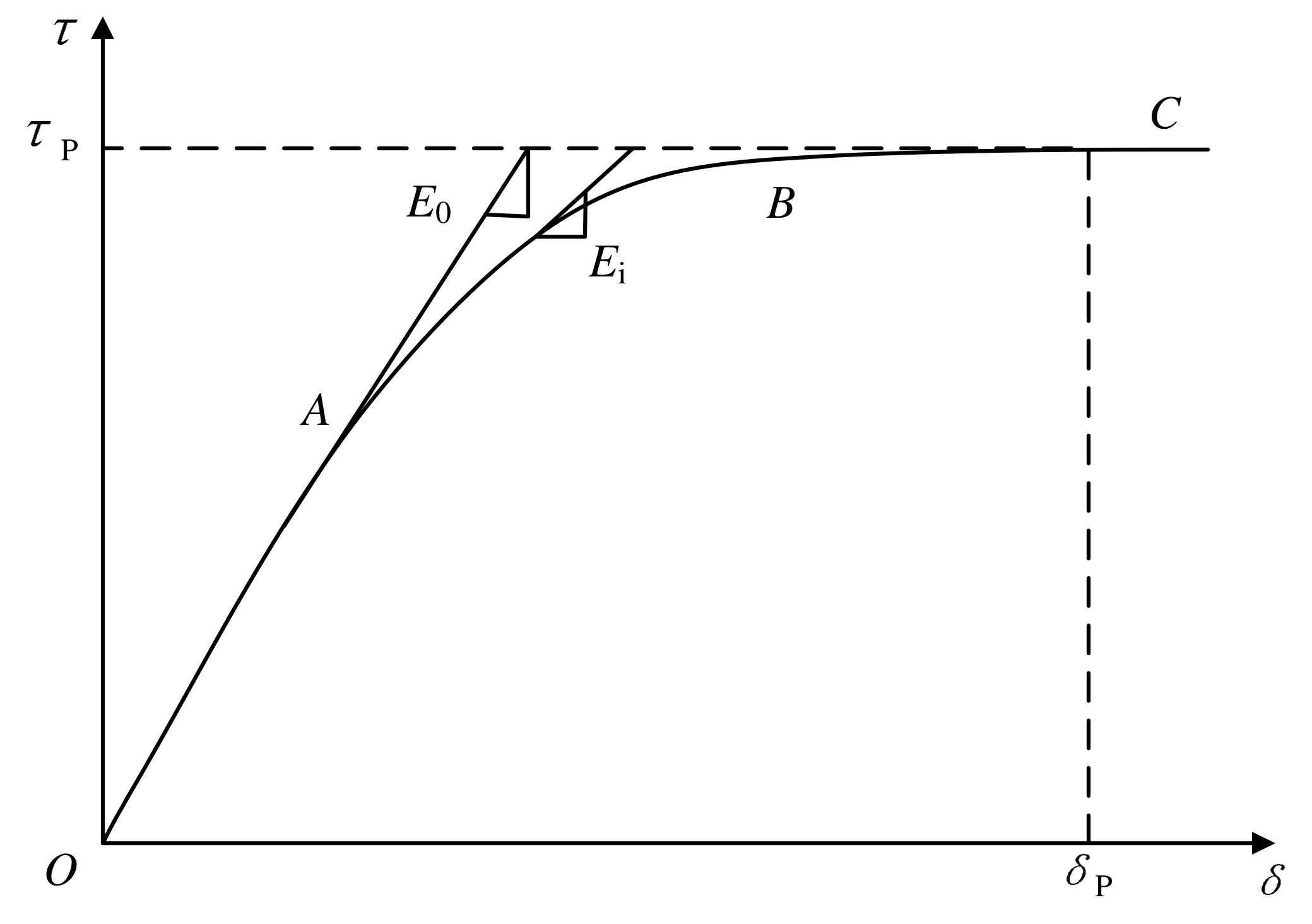
The typical shear stress-shear strain (τ-δ) curve for strain-hardening behavior of Nmcs is shown in Figure 1. As can be seen, the strain-hardening process can be divided into three stages: elastic stage (OA), plastic stage (AB), and failure stage (BC). In the elastic stage, the τ-δ curve shows a straight line and the shear stress increases linearly with the shear strain at a gradient of initial elastic modulus E₀. In the plastic stage, the tangent modulus E_i reduces gradually as strain accumulates, leading to a nonlinear τ-δ curve. In the failure stage, the τ-δ curve flattens out and the shear stress reaches the ultimate shear strength τ_p with a corresponding shear strain δ_p. In this stage, the shear stress is mainly contributed by the friction resistance at the failure surface of the soil sample. In sum, the strain-hardening curve includes four mathematical features: through the origin, monotone increasing, convex to τ-axis, and infinite convergence.

2.2.2. Falling τ-δ Behavior

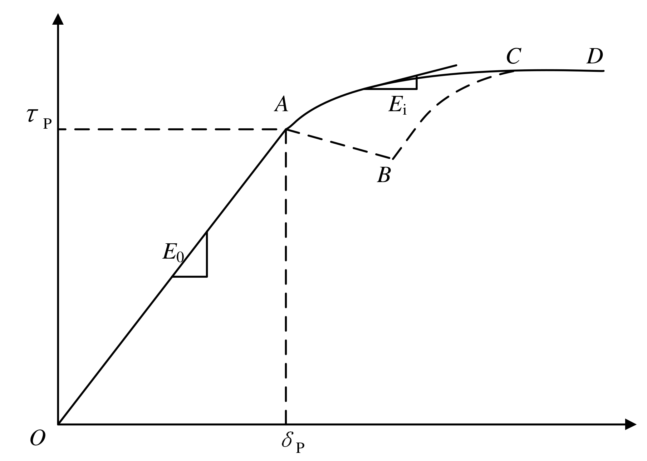
In the direct shear test of seashore soft soil after adding Nm, the cohesive force was lost after failure and hence the shear stress decreased dramatically. The falling τ-δ curve after the elastic stage shows an evident softening behavior. As shown in Figure 2, the typical τ-δ curve can be divided into four stages. Stage 1 is the elastic stage (OA) which is similar to that of strain-hardening curve. In this stage, the shear stress increases with the gradient of initial elastic modulus until reaching the failure. The corresponding shear stress and strain at point A denote the failure displacement δ_p and shear strength τ_p, respectively. Stage 2 is the falling stage (AB), which evidently shows the falling of shear stress after the soil fails. This falling of shear stress is attributed to the loss of cohesion and the tangent modulus of the τ-δ curve gives a negative value. Stage 3 is the plastic stage (BC) wherein the friction resistance starts to dominate after the loss of cohesion. In this stage, the tangent modulus of the curve approximates the initial elastic modulus at the beginning which subsequently decreases due to the occurrence of plastic shear stress. Stage 4 is the residual shear stress stage (CD) where the tangent modulus approaches zero and the shear stress is equal to residual shear stress. It should be noted that the τ-δ falling curve can be modified by ignoring Stages 2 and 3 (AB and BC), then it returns to the strain-hardening behavior. However, the shear strength in the falling curve refers to the shear stress at the end of Stage 1 which is different from its counterpart in the strain-hardening curve.

2.2.3. S-Type Falling τ-δ Behavior

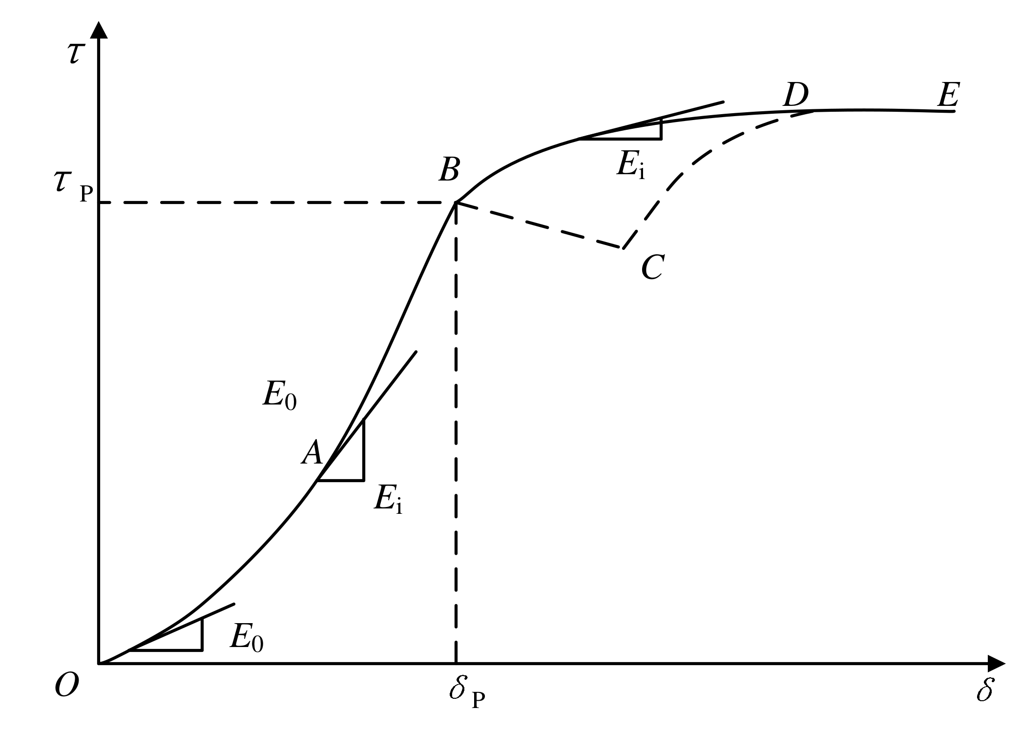
Based on the τ-δ response of Nmcs in the scenario with high corrosion, the typical S-type falling curve is shown in Figure 3. As can be seen, the S-type falling curve consists of five stages. Stage 1 refers to the erosion softening stage (OA) where the surface of the sample is eroded by highly corrosive sulfuric acid and becomes relatively soft. Initially, the increment in the shear stress is relatively small as the displacement increases, giving rise to a relatively small initial modulus. As the shearing develops and enters the hard soil, which is less corroded, the tangent modulus tends to increase until stabilizing when accessing Stage 2, i.e., linear elastic stage (AB). The shear strength τ_p and corresponding displacement δ_p at failure occur at the end of Stage 2, i.e., point B. After reaching failure, the falling stage (BC), the frictional plastic stage (CD) and the residual shear stress stage (DE) emerge continuously. These three stages are similar to those in the above falling behavior. Thus, the S-type falling curve can be modified in a similar way as that for the above falling curve. However, the obtained modified curve is still unlike the strain-hardening curve which is convex to τ-axis; namely, an inflection point occurs on the curve, e.g., before this point, the curve is convex to δ-axis, while after this point, it is convex to τ-axis.

2.3. Mathematical Characteristics of σ-δ Behavior

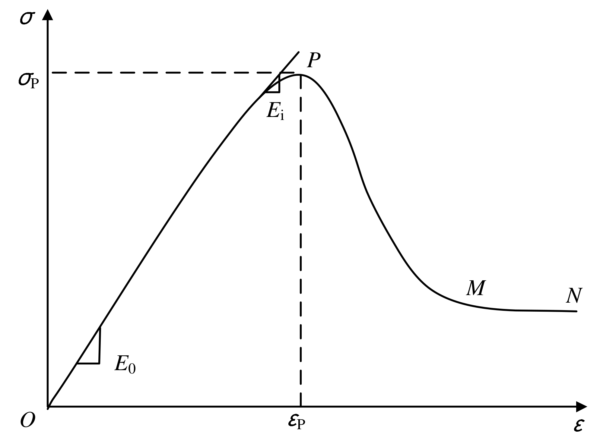
Based on the UCS (unconfined compression strength test) results, the stress–strain curve under uniaxial compression exhibits a strong softening and brittle failure behavior, as shown in Figure 4. As can be seen, the stress–strain curve is hump-shaped where the peak point of the curve gives the unconfined compressive strength σ_p corresponding to a strain of ε_p. This curve comprises three stages. In the hardening stage (OP), the stress initially increases linearly with strain; the gradient of which represents the initial elastic modulus E₀. This gradient starts to decrease in the later phase of the hardening stage until arriving at the peak, i.e., point P where the brittle failure takes place and the tangent modulus equals to zero. After that the stress reduces monotonically with strain in the softening stage (PM) and remains unchanged when entering the residual stress stage (MN). In sum, the mathematical features of the curve include: through the origin, having extreme value point, and converging at residual stress.

3. Established Mathematical Model

The characteristics of modified falling τ-δ curve are almost consistent with those of strain-hardening τ-δ curve. Therefore, this study attempts to establish a simple, mathematical constitutive model which is applicable for modeling both strain-hardening and modified falling τ-δ behaviors of Nmcs.

3.1. Conventional Shear Stress-Displacement (τ-δ) Models

The conventional shear stress-displacement models have three types: hyperbolic model, exponential model and power function model.

3.1.1. Hyperbolic Model

The most classical nonlinear model describing hardening curve is hyperbolic model, which is widely applied to the nonlinear modeling in various fields because of its simple expression, convenient simulation and easy determination of parameters. The hyperbolic model was proposed by Duncan and Chang [40] and its expression is

$$\tau =\frac{\delta }{1/E_0+\delta /{\tau }_{\mathrm{p}}},$$

(1)

where τ is the shear stress (kPa), δ is the shear displacement (mm), E₀ is the nominal elastic modulus (kPa/mm) and τ_p is the shear strength (kPa).

According to the τ-δ curves of shear test on the soil-structure contact surface, the hardening curve is rigid and plastic, and the hyperbolic model is difficult to meet this condition. In contrast, the strain in the τ-δ curve of Nmcs is mostly elastic before failure and only a small amount of plastic strain occurs after failure. In addition, the hyperbolic curve produces a large error in fitting the softening curve, which causes the deviation between the fitting results and the measured data due to its mathematical characteristics. Therefore, the hyperbolic model may be not suitable for modeling both hardening and softening behaviors.

3.1.2. Exponential Model

The exponential model converges faster, and it is suitable for the τ-δ curves with elastoplastic strain. Hence, it is superior to the hyperbolic model for hardening curves. The exponential model was firstly proposed based on the one-dimensional consolidation theory of Terzaghi, and was mainly applied to describe the stress–strain curve of soil. The mathematical constitutive function is

$$\tau ={\tau }_{\mathrm{p}}\left(1-e^{-E_0\delta /{\tau }_{\mathrm{p}}}\right).$$

(2)

Cai et al. [41] investigated the mathematical defects of the exponential model using the half-value strength index. The results showed that the half-value strength index of both the exponential and the hyperbolic function is a fixed value which is only related to the peak strength and the initial elastic modulus. In this regard, the simulated stress–strain curve is only applicable for specific cases. In contrast, the half-value strength index of the power function is a parameter with a non-fixed value. The shape of its curve varies with the variation of the parameters, and hence it is widely applicable.

3.1.3. Power Function Model

Due to the mathematical characteristics of the power function model, its simulation effect is remarkable in modeling plastic curves. In addition, the power function model of the nonlinear constitutive model of clay has the parameter of tangent modulus index. The expression of the power function model is

$$\tau ={\tau }_{\mathrm{p}}\left\{1-{\left[1+\frac{\left(\theta -1\right)E_0}{{\tau }_{\mathrm{p}}}\delta \right]}^{\frac{1}{1-\theta }}\right\},$$

(3)

where the value of θ is larger than 1; when θ = 2, the power function becomes the hyperbolic shear stress-displacement constitutive equation, so the hyperbolic function is only a special case of the power function. The first derivative of Equation (3) is given as

$$\frac{d\tau }{d\delta }=E_0{\left[1+\frac{\left(\theta -1\right)E_0}{{\tau }_{\mathrm{p}}}\delta \right]}^{\frac{\theta }{1-\theta }}.$$

(4)

Since θ > 1, the first derivative of the power function is always greater than 0 in the domain of definition, and the curve increases monotonically. As the parameter θ changes, it is more applicable to the hardening curve and modified falling curve.

The second derivative of Equation (3) leads to

$$\frac{d^2\tau }{d{\delta }^2}=-\frac{E_0{}^2\theta }{{\tau }_{\mathrm{p}}}{\left[1+\frac{\left(\theta -1\right)E_0}{{\tau }_{\mathrm{p}}}\delta \right]}^{\frac{2\theta -1}{1-\theta }}.$$

(5)

It can be found that the second derivative of power function is always less than zero, meeting the characteristic of hardening and modified falling curves, i.e., convex to τ-axis. However, the inflection point occurs on the S-type τ-δ curve under a highly corrosive environment. Therefore, the second derivative of power function cannot be equal to zero.

3.2. Mathematical REP Model for τ-δ Behavior

Based on the above conventional mathematical models, a new REP (reinforced exponential and power function) mathematical model for modeling the shear stress-displacement behavior of Nmcs under acid erosion environment is proposed in this study. This model combines exponential and power functions, which is expressed as

$$\tau =a\left[1-e^{-b\delta }{\left(1+k\delta \right)}^{-\lambda }\right],$$

(6)

where a, b, λ, and k are parameters to be determined, and a ≥ 0, b > 0, λ > 0, k > 0. When k = 0, Equation (6) degrades into exponential function.

Taking the limit and the first derivative of Equation (6) leads to

$$\left\{\begin{array}{l}\tau \left|{}_{\delta =+\infty }\right.=a\hfill \\ \frac{d\tau }{d\delta }=ab{e}^{-b\delta }{\left(1+k\delta \right)}^{-\lambda }+a\lambda k{e}^{-b\delta }{\left(1+k\delta \right)}^{-\lambda -1}\hfill \end{array}\right..$$

(7)

The progressive limit of τ-δ curve is shear strength, i.e., τ_p. Hence,

$$a={\tau }_{\mathrm{p}}.$$

(8)

The first derivative of the new model with δ=0 is the initial modulus of elasticity, i.e., E₀. Combining with Equation (8) gives

$${\tau }_{\mathrm{p}}b+{\tau }_{\mathrm{p}}\lambda k=E_0,$$

(9)

where

$$b=\frac{E_0}{{\tau }_{\mathrm{p}}}-\lambda k.$$

(10)

According to Equation (10), (E₀/τ_p − λk) > 0 if b > 0.

Based on the above, the REP model for the hardening τ-δ curve can be expressed as

$$\tau ={\tau }_{\mathrm{p}}\left[1-e^{-\left(E_0/{\tau }_{\mathrm{p}}-\lambda k\right)\delta }{\left(1+k\delta \right)}^{-\lambda }\right].$$

(11)

In order to analyze whether REP model satisfies the mathematical characteristics of hardening curve, the zero point, the limit, the first derivative and the second derivative are discussed as below

$$\left\{\begin{array}{l}\tau \left|{}_{\delta =0}=0\right.\\ \tau \left|{}_{\delta =+\infty }={\tau }_{\mathrm{p}}\right.\\ \frac{d\tau }{d\delta }=E_0\left(E_0/{\tau }_{\mathrm{p}}-\lambda k\right)e^{-\left(E_0/{\tau }_{\mathrm{p}}-\lambda k\right)\delta }{\left(1+k\delta \right)}^{-\lambda }+E_0\lambda k{e}^{-\left(E_0/{\tau }_{\mathrm{p}}-\lambda k\right)\delta }{\left(1+k\delta \right)}^{-\lambda -1}\\ \frac{d^2\tau }{d{\delta }^2}=-E_0{\left(E_0/{\tau }_{\mathrm{p}}-\lambda k\right)}^2{e}^{-\left(E_0/{\tau }_{\mathrm{p}}-\lambda k\right)\delta }{\left(1+k\delta \right)}^{-\lambda }\\ -2E_0\left(E_0/{\tau }_{\mathrm{p}}-\lambda k\right)\lambda k{e}^{-\left(E_0/{\tau }_{\mathrm{p}}-\lambda k\right)\delta }{\left(1+k\delta \right)}^{-\lambda -1}-E_0\lambda \left(\lambda +1\right)k^2{\left(1+k\delta \right)}^{-\lambda -1}\end{array}\right.$$

(12)

When δ = 0, the shear stress equals to 0 so the curve passes through the origin, satisfying the first characteristic of the hardening curve. The coefficients in the first-order derivative equation are all positive, and the first-order derivative is always greater than 0 in the domain of definition, which satisfies the characteristic of monotonic increase. When the displacement δ approaches infinity, shear stress gradually gets close to shear strength of τ_p. Therefore, the new model goes through the origin and has both upper and lower bounds. The coefficients of the second derivative equation are all negative, and the second derivative of the new model is always less than 0. Hence, the REP model is theoretically suitable for the hardening and modified falling curves.

3.3. Mathematical Models for Stress-Displacement (σ-δ) Behavior

Likewise, the conventional mathematical model for the constitutive relation of stress- displacement (σ-δ) behavior also has many types such as hyperbolic, exponential function, power function, piecewise function and quadratic function. As aforementioned, the power function model has a better fitting effect than hyperbolic and exponential functions, while the piecewise function has some defects, e.g., it is troublesome to fit and has many parameters. Therefore, in the study of models for stress-displacement (σ-δ) behavior, only power function, quadratic function, and the proposed REP function are discussed.

For the power function of σ-δ behavior, it can be easily modified from Equation (3), that is

$$\sigma ={\sigma }_{\mathrm{p}}\left\{1-{\left[1+\frac{\left(\theta -1\right)E_0}{{\sigma }_{\mathrm{p}}}\epsilon \right]}^{\frac{1}{1-\theta }}\right\},$$

(13)

where ε is the strain (%), σ is the stress (kPa) and σ_p is the peak value of the stress–strain curve (UCS).

The quadratic model is able to simulate the stress–strain curve of compacted cement soil with an obvious peak value; its expression is

$$\sigma ={\sigma }_{\mathrm{p}}\left[A\frac{\epsilon }{{\epsilon }_{\mathrm{p}}}-B{\left(\frac{\epsilon }{{\epsilon }_{\mathrm{p}}}\right)}^2\right],$$

(14)

where σ_p and ε_p are the maximum stress and the corresponding strain, respectively. A and B are the fitting parameters to be determined.

When ε = 0, the stress of power and quadratic models is 0, which satisfies the characteristic of the stress–strain curve passing through the origin. As aforementioned, in the process of power function fitting, it is unable to converge in the failure stage, while the strong softening stress–strain curve will soften immediately after reaching the peak failure. Therefore, the convergence of the power function may be not timely, which may lead to a large deviation from the measured curve. Although the quadratic model is able to converge in time after the peak value; when the strain approaches infinity, the stress is also infinite, which theoretically does not meet the characteristics of infinite convergence of the stress–strain curve.

The expression of REP model for the σ-δ behavior is slightly different from that for the τ-δ behavior, i.e., Equation (11)

$$\sigma =a\left[1-e^{-b\epsilon }{\left(1+k\epsilon \right)}^{-\lambda }\right],$$

(15)

where a, b, λ, and k are parameters to be determined, and the value range of each parameter should be suitable for the hump curve. When ε = 0, the σ value of the REP model also equals to zero which satisfies the characteristic of passing through the origin.

The first and second derivatives of the stress–strain curve are as follows

$$\left\{\begin{array}{l}\frac{d\sigma }{d\delta }=ab{e}^{-b\epsilon }{\left(1+k\epsilon \right)}^{-\lambda }+a\lambda k{e}^{-b\epsilon }{\left(1+k\epsilon \right)}^{-\lambda -1}\hfill \\ \frac{d^2\sigma }{d{\delta }^2}=-a{b}^2{e}^{-\left(E_0/{\tau }_{\mathrm{p}}-\lambda k\right)\delta }{\left(1+k\epsilon \right)}^{-\lambda }-2ab\lambda k{e}^{-b\epsilon }{\left(1+k\epsilon \right)}^{-\lambda -1}-a\lambda \left(\lambda +1\right)k^2{\left(1+k\epsilon \right)}^{-\lambda -1}\hfill \end{array}\right..$$

(16)

It can be observed that the first and second derivatives of REP model are affected by the value of each parameter, and the positive and negative signs are uncertain which enables its adaptability to complex strain-softening curves. The specific value range of each parameter and the judgment of the positive and negative sign of the first derivative and the second derivative need further study.

3.4. Application and Analysis

3.4.1. Hardening τ-δ Behavior

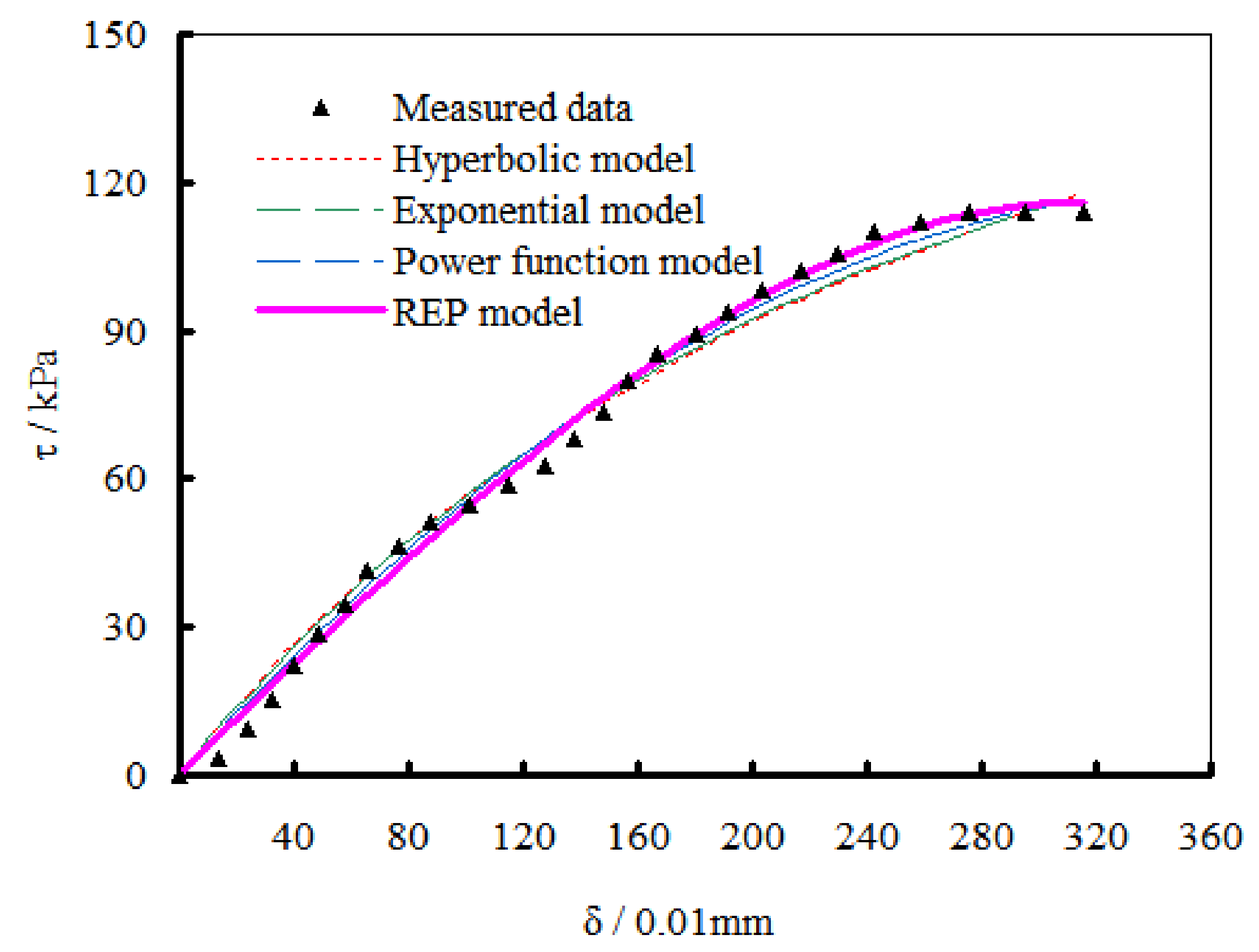
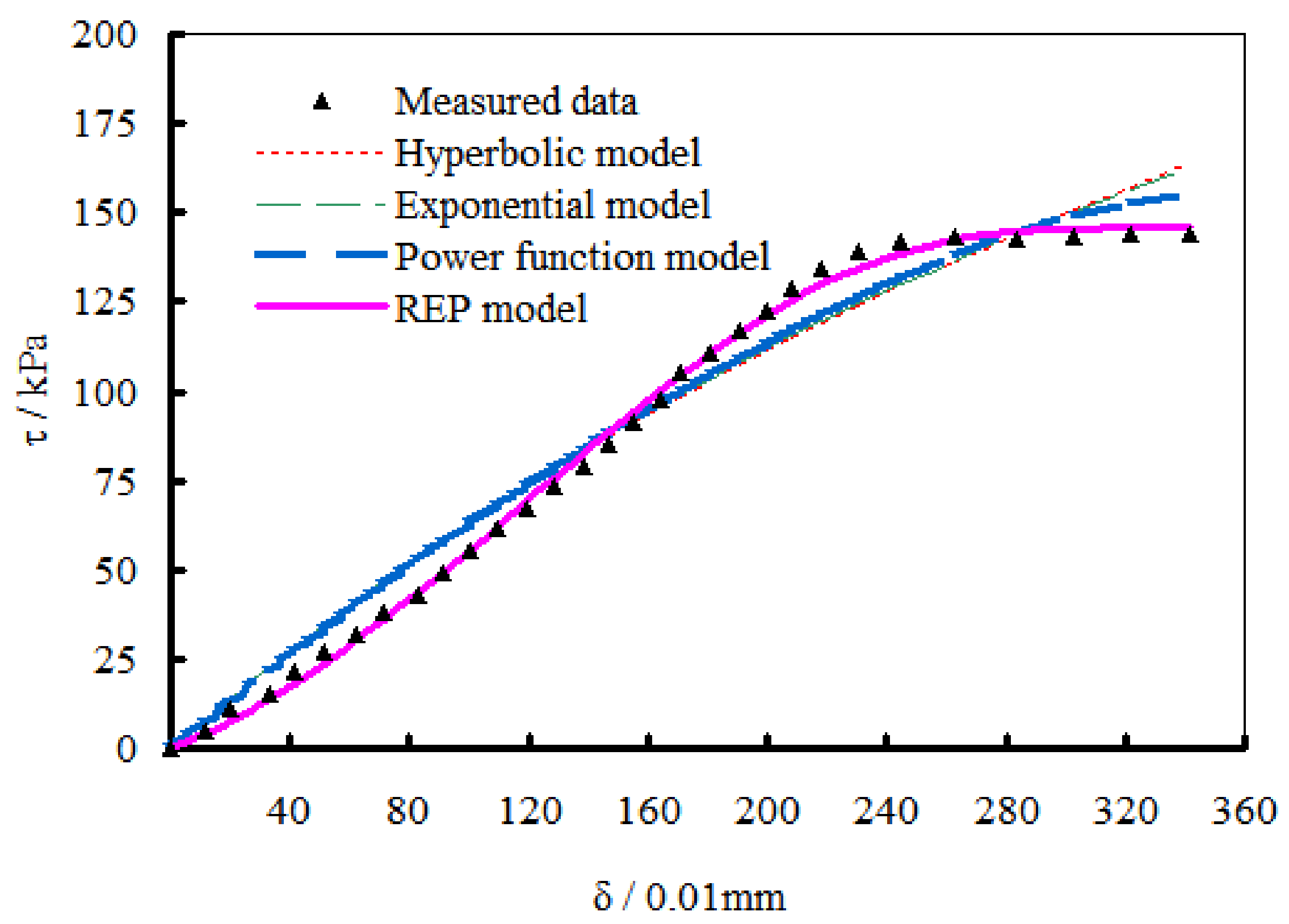
Based on the measured data of direct shear test, comparisons of using hyperbolic, exponential and power function models as well as the proposed REP model are made. Two cases with 5% and 7% cement mixture ratio were examined. To determine the aforementioned model parameters, e.g., λ and k, four tests with vertical pressures of 100, 200, 300, and 400 kPa were carried out respectively. The comparison results for the cases under a vertical pressure of 400 kPa are shown in Figure 5 and Figure 6.

As shown in Figure 5, on the whole, the four models have a good fitting effect, but the elastic stage of the measured curve is not smooth, and there is a prominent inflection point locally. In this stage, the four models have a large deviation from the measured value. The tangent modulus of the measured curve decreases gradually in the plastic stage, and the hyperbolic, exponential and power functions converge slowly, all of which appear below the curve while the fitting effect of REP model is very evident. When entering failure stage, both the hyperbolic and exponential fittings cannot converge to τ_p, and lie in the upper part of the measured curve with big difference. In contrast, the power function converges well, and the fitting effect is better than the hyperbolic and exponential functions, although the end of the curve still appears above the measured curve. The REP model also has a good convergence effect and the whole fitted failure stage is very close to that of the measured curve.

As shown in Figure 6, the linearity of the measured curve in the elastic stage is not obvious while the hyperbolic, exponential, and power function curves are linear, deviating slightly from the measured curve. In the plastic deformation stage, the three functions appear below the measured curve, and the difference between the power function and the measured curve is the smallest. Similar to that observed in Figure 5, in the failure stage, the three models generally appear at the top of the curve. In contrast, the REP model is very close to the measured curve and shows an evidently favorable fitting effect.

Among the conventional models, the power function model is relatively superior in modeling τ-δ curves, particularly in the plastic stage where the computed results are closer to the measured curve and failure, and in the failure stage showing a faster convergence speed. Compared with the hyperbolic model, the exponential model has a better simulation effect. Moreover, the REP model shows superior fitting accuracy than the conventional mathematical models.

3.4.2. Modified Falling τ-δ Behavior

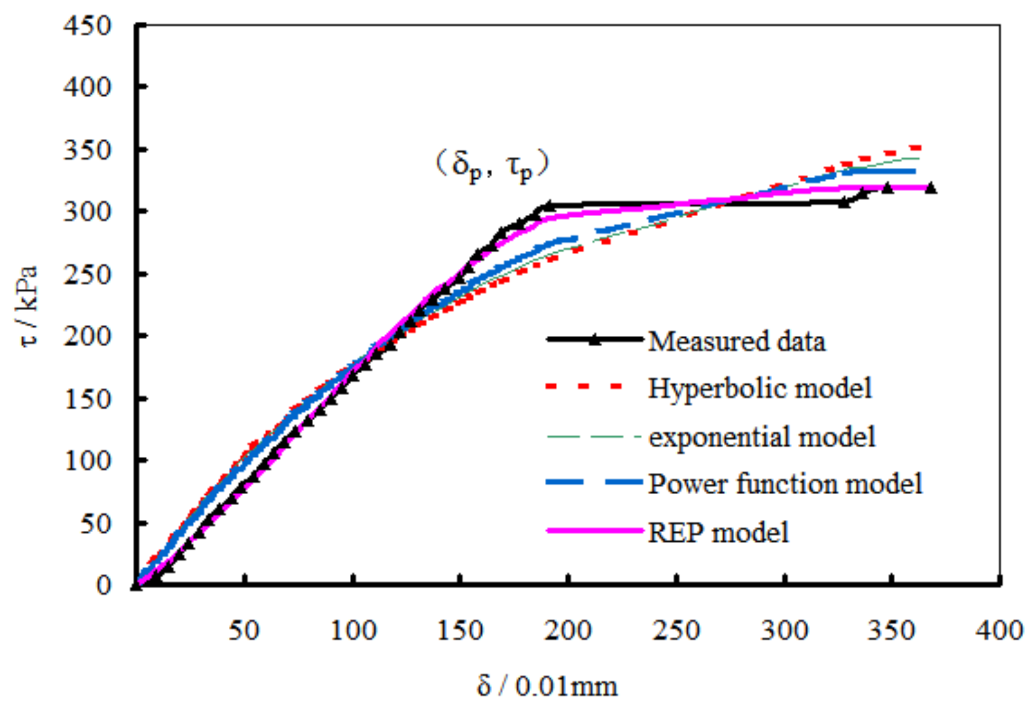
After adding Nm, the τ-δ curve exhibits modified falling type. In the comparison of different mathematical models, two cases with Nm mixing ratios of 10‰ and 20‰ under a vertical pressure of 400kPa were selected. The results are shown in Figure 7 and Figure 8.

As can be seen, the shape of the two measured curves is similar. Before failure, the modified curve is mostly elastic stage and there is no plastic transition stage showing significant linearity. In this stage, the conventional models produce non-linear curves, while the measured curve approximates a horizontal line in the failure stage. The curves of conventional models locate below the measured curve in the former part and above the measured curve in the later part. In the two stages, the conventional model intersects with the measured curve, exhibiting two “X” shapes. In general, the difference between conventional models and measured curve is relatively big while the REP model fits fairly well with the measured curve. Therefore, the proposed REP model has significant advantage in modeling the modified τ-δ curve. In contrast, it is easy for a double-“X” type discrepancy to appear in the conventional mathematical model simulation.

3.4.3. Strong Softening σ-δ Behavior

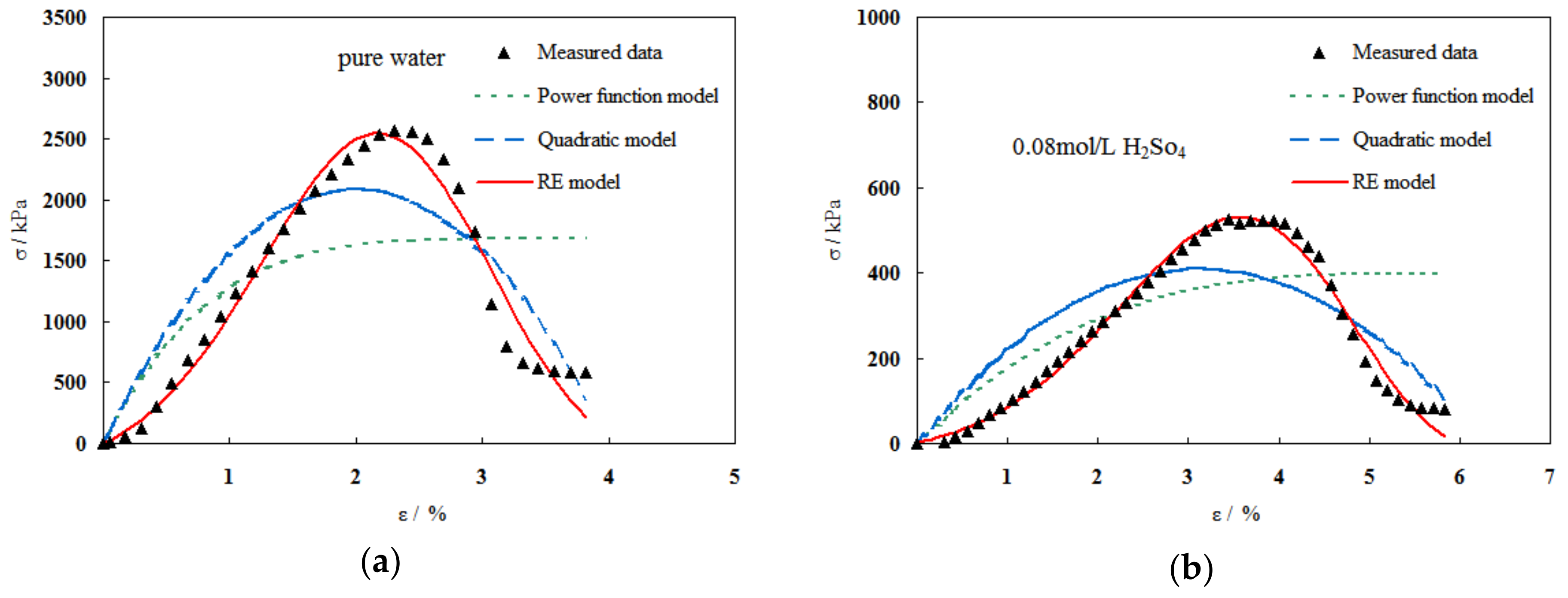
To compare the performance of the power function and quadratic function models as well as the REP model, UCS experimental results for cases with 0 mol/L and 0.08 mol/L H₂SO₄ erosion were adopted, Figure 9. As can be seen, the power function model behaves the worst in the modeling of the hump-shaped σ-δ curve. For instance, it is convex at the rising stage of the curve, which is contrary to the characteristic of concave in the measured curve. In addition, it cannot simulate the softening behavior as the measured curve although it converges to an almost constant value in the end. The quadratic function model performs better than the power function model. It is able to simulate the softening behavior and give a peak stress value. However, the shape of the quadratic curve is convex in all stages, which differs with the shape of measured curves. Worse still, there exists a large discrepancy in the maximum stress value and its corresponding strain value between the results of quadratic model and the measured results. This may raise an adverse effect in predicting UCS results. In contrast, the results of proposed REP model agree incredibly well with the measured results. The REP model not only shows consistent shapes, but also predicts a fairly close maximum stress value and a corresponding strain value. This is of great engineering value in predicting the compressive strength.

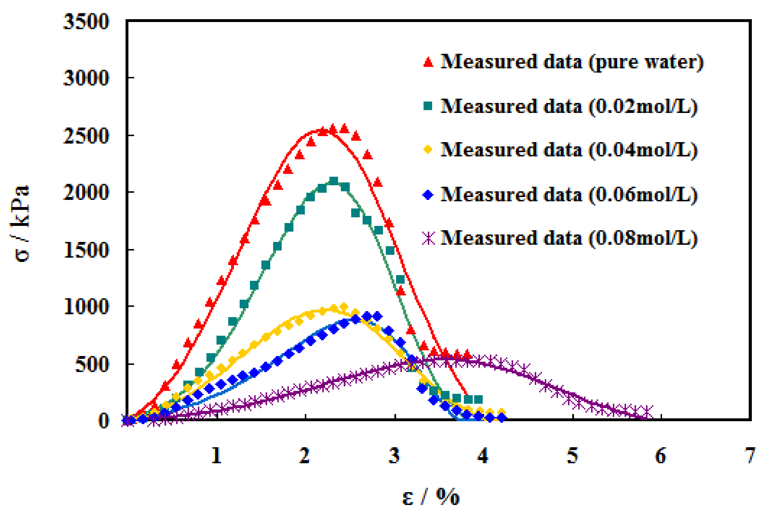
To further examine the performance of the REP model, a series of comparisons for cases with varying erosion concentrations (i.e., 0.00 mol/L, 0.02 mol/L, 0.04 mol/L, 0.06 mol/L and 0.08 mol/L) is conducted, Figure 10. As can be seen, in the stress rising stage, the REP model fits fairly well with measured results; in the reducing stage, slight discrepancy occurs for the cases with 0.00 mol/L and 0.02 mol/L erosion concentrations. This could be attributed to the scattered data of the measured results. In the final residual stage, the REP model deviates from the measured data when the convergent residual stress was relatively large, such as the cases in pure water (i.e., 0.00 mol/L) and 0.02 mol/L acid erosion environment. When the residual stress was relatively small in the environment with a high concentration of acid erosion, the REP model gives better performance in fitting. Therefore, it can be found that the REP model can adapt to the measured curve under different acid erosion concentrations, with relatively high fitting accuracy. The fitting effect is more evident under a high concentration erosion environment.

Table 1. Four parameter values of REP model under different erosion concentrations.

H2SO4 Erosion Concentrations	Parameter
	a	b	k	λ
0.00 mol/L	223.23	16.62	0.08	131.20
0.02 mol/L	83.33	5.95	0.18	19.76
0.04 mol/L	100.70	7.53	0.12	48.53
0.06 mol/L	79.73	2.36	0.25	3.60
0.08 mol/L	40.00	2.93	0.12	14.04

provides the values of the four parameters in the REP model for these five cases.

In order to study the influence of erosion concentration on REP model parameters, an acid erosion factor was introduced

$$\omega \left(x,y,z,a_s\right)=\frac{{\pi }^{2}x}{2\pi y+4z{a}_s},$$

(17)

where x, y, and z are the parameters to be determined; α_s is the concentration of sulfuric acid solution.

In accordance with Table 1, substituting the acid erosion factor and acid erosion concentration α_s into the four parameters of REP model leads to

$$\left\{\begin{array}{l}a=8\phi \tan \left[{\omega }_a\left(a_s\right)+1.84c\right]-1.84c\hfill \\ b=-0.45c-2.18\phi \cos \left[{\omega }_b\left(a_s\right)+2.18\phi \right]\hfill \\ k=0.11\tan \left[{\omega }_k\left(a_s\right)+0.16\right]-0.16\hfill \\ \lambda =-2.2c-a_s-2.1c\sin \left[{\omega }_{\lambda }\left(a_s\right)+2.2c\right]\hfill \end{array}\right.,$$

(18)

where c and φ are the cohesion and internal friction angle of silty clay in the experiment, respectively.

Hence, the acid erosion factors of the four parameters can be obtained

$$\left\{\begin{array}{l}{\omega }_a\left(a_s\right)=\omega \left(-7.96\phi ,0.881,1.84c,a_s\right)\hfill \\ {\omega }_b\left(a_s\right)=\omega \left(2.18217\phi ,-0.100816,0.44586c,a_s\right)\hfill \\ {\omega }_k\left(a_s\right)=\omega \left(0.1111,-6.592\phi \times {10}^{-6},0.158,a_s\right)\hfill \\ {\omega }_{\lambda }\left(a_s\right)=\omega \left(2.095c,2.1927c,-105.507c,a_s\right)\hfill \end{array}\right..$$

(19)

Combining with Equations (15) and (19), the damage model of sulfuric acid erosion can be expressed as

$$\sigma =a_{\left[{\omega }_a\left(a_s\right),a_s\right]}\left[1-e^{-b_{\left[{\omega }_b\left(a_s\right),a_s\right]}\epsilon }{\left(1+k_{\left[{\omega }_k\left(a_s\right),a_s\right]}\epsilon \right)}^{-{\lambda }_{\left[{\omega }_{\lambda }\left(a_s\right),a_s\right]}}\right].$$

(20)

As shown in Equation (20), the damage model only contains parameters of sulfuric acid concentration (α_s), cohesion (c) and internal friction angle (φ), making the new model more suitable for acid erosion environment.

4. Mathematical CEL Model for Modified S-Type Falling τ-δ Behavior

As discussed above, the REP model has fairly good fitting effect which can be used for different types of stress–strain curves. However, for the S-type curve which has inflection points, it is time-consuming to calculate the zero point of the second derivative equation of REP model and determine the position of inflection points. To solve this, the REP is therefore simplified and a new CEL (coupled exponential and linear) model is put forth.

4.1. Mathematical CEL Model

The CEL model is actually a coupled exponential and linear function model.

Setting λ = −1, Equation (6) can be simplified as

$$\tau =a\left[1-e^{-b\delta }\left(1+k\delta \right)\right],$$

(21)

where α ≥ 0, b > 0 and k > 0; k is defined as the inflection factor.

Taking the limit of Equation (21) gives

$$\tau \left|{}_{\delta =+\infty }\right.=a\left[1-e^{-b\delta }\left(1+k\delta \right)\right]\left|{}_{\delta =+\infty }\right.=a\left(1-0\right)=a.$$

(22)

Since the S-type curve eventually converge to the shear strength τ_p so

$$a={\tau }_{\mathrm{p}}.$$

(23)

Taking the first derivative of Equation (21) leads to

$$\frac{d\tau }{d\delta }=ab{e}^{-b\delta }\left(1+k\delta \right)-ak{e}^{-b\delta }.$$

(24)

If δ = 0, then

$$\frac{d\tau }{d\delta }\left|{}_{\delta =0}\right.=a\left(b-k\right).$$

(25)

The first derivative of the new model is the initial elastic modulus when the displacement is 0, i.e., δ = 0. Combining with Equation (23) gives

$${\tau }_{\mathrm{p}}\left(b-k\right)=E_0.$$

(26)

Hence, the parameter b can be derived

$$b=\frac{E_0}{{\tau }_{\mathrm{p}}}+k,$$

(27)

and the CEL model can be expressed as

$$\tau =E_0\left[1-e^{-\left(\frac{E_0}{{\tau }_{\mathrm{p}}}+k\right)\delta }\left(1+k\delta \right)\right].$$

(28)

In order to explore whether the CEL model satisfies the mathematical characteristics of the S-type curve, its zero point, limit, first derivative, and second derivative are discussed

$$\left\{\begin{array}{l}\tau \left|{}_{\delta =0}=E_0\left[1-1\cdot \left(1-0\right)\right]=0\right.\hfill \\ \tau \left|{}_{\delta =+\infty }={\tau }_{\mathrm{p}}\right.\hfill \\ \frac{d\tau }{d\delta }={\tau }_{\mathrm{p}}\left(\frac{E_0}{{\tau }_{\mathrm{p}}}+k\right)e^{-\left(\frac{E_0}{{\tau }_{\mathrm{p}}}+k\right)\delta }\left(1+k\delta \right)-{\tau }_{\mathrm{p}}k{e}^{-\left(\frac{E_0}{{\tau }_{\mathrm{p}}}+k\right)\delta }\hfill \\ \frac{d^2\tau }{d{\delta }^2}=-{\tau }_{\mathrm{p}}{\left(\frac{E_0}{{\tau }_{\mathrm{p}}}+k\right)}^2{e}^{-\left(\frac{E_0}{{\tau }_{\mathrm{p}}}+k\right)\delta }\left(1+k\delta \right)+2{\tau }_{\mathrm{p}}\left(\frac{E_0}{{\tau }_{\mathrm{p}}}+k\right)k{e}^{-\left(\frac{E_0}{{\tau }_{\mathrm{p}}}+k\right)\delta }\hfill \end{array}\right..$$

(29)

According to Equation (29), the CEL model goes through the origin and converges to τ_p at infinity. Combining the similar items in the first derivative of Equation (29) gives

$$\frac{d\tau }{d\delta }=\left(E_0+E_{0}k\delta +{\tau }_{\mathrm{p}}{k}^2\delta \right)e^{-\left(\frac{E_0}{{\tau }_{\mathrm{p}}}+k\right)\delta }>0.$$

(30)

Hence, the first derivative of CEL model is always greater than 0 in the domain of definition, and the curve increases monotonically.

The displacement at zero point of the second derivative of Equation (29) is obtained by

$${\delta }_c=\frac{{\tau }_{\mathrm{p}}k-E_0}{{\tau }_{\mathrm{p}}{k}^2+E_{0}k}.$$

(31)

To analyse the concavity of CEL model at zero point of second derivative, the relations are

$$\left\{\begin{array}{c}\frac{d^2\tau }{d{\delta }^2}>0,\left(\delta <\frac{{\tau }_{\mathrm{p}}k-E_0}{{\tau }_{\mathrm{p}}{k}^2+E_{0}k}\right)\\ \frac{d^2\tau }{d{\delta }^2}<0,\left(\delta >\frac{{\tau }_{\mathrm{p}}k-E_0}{{\tau }_{\mathrm{p}}{k}^2+E_{0}k}\right)\end{array}\right..$$

(32)

When δ < δ_c, τ’’ > 0 and the curve is convex to the δ-axis; when δ > δ_c, τ’’ < 0 and the curve is convex to the τ-axis.

4.2. Application and Analysis

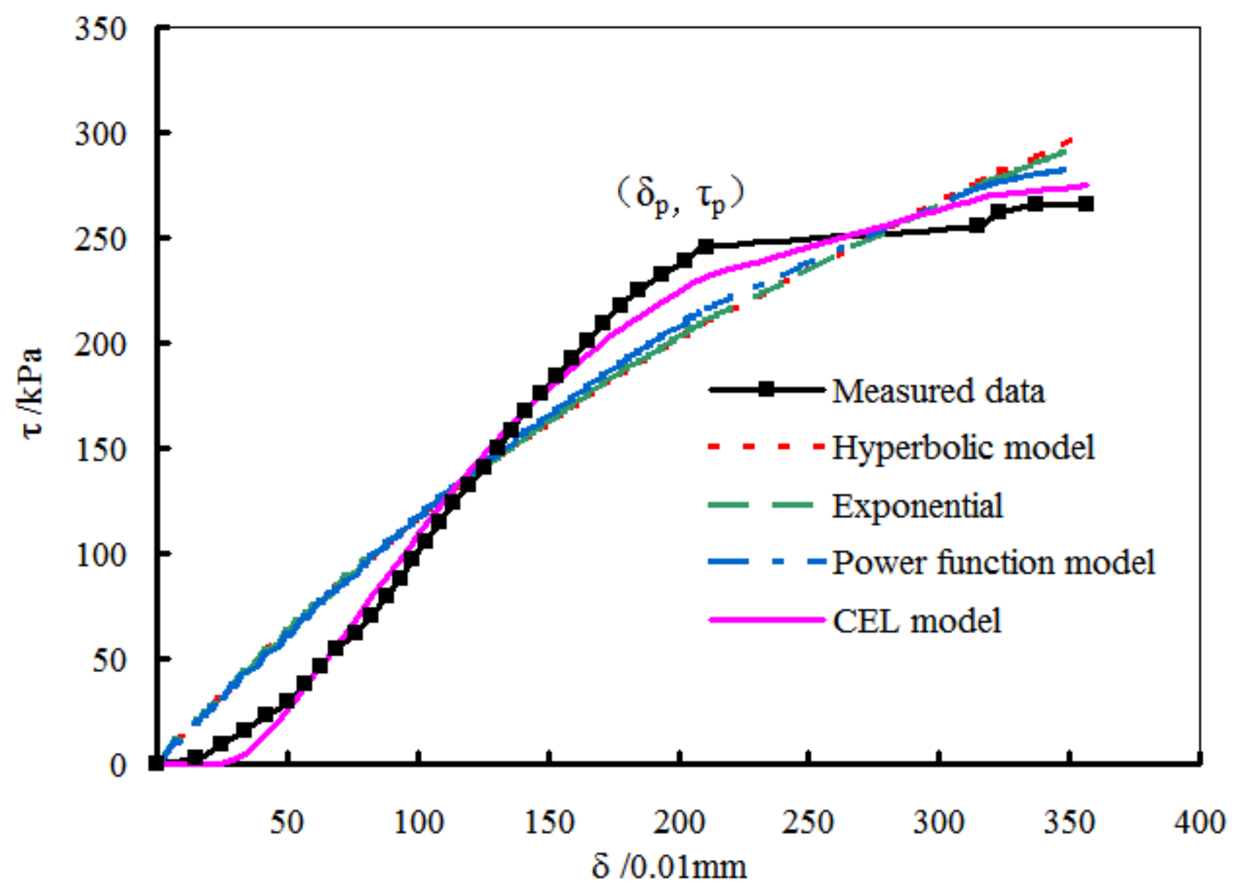
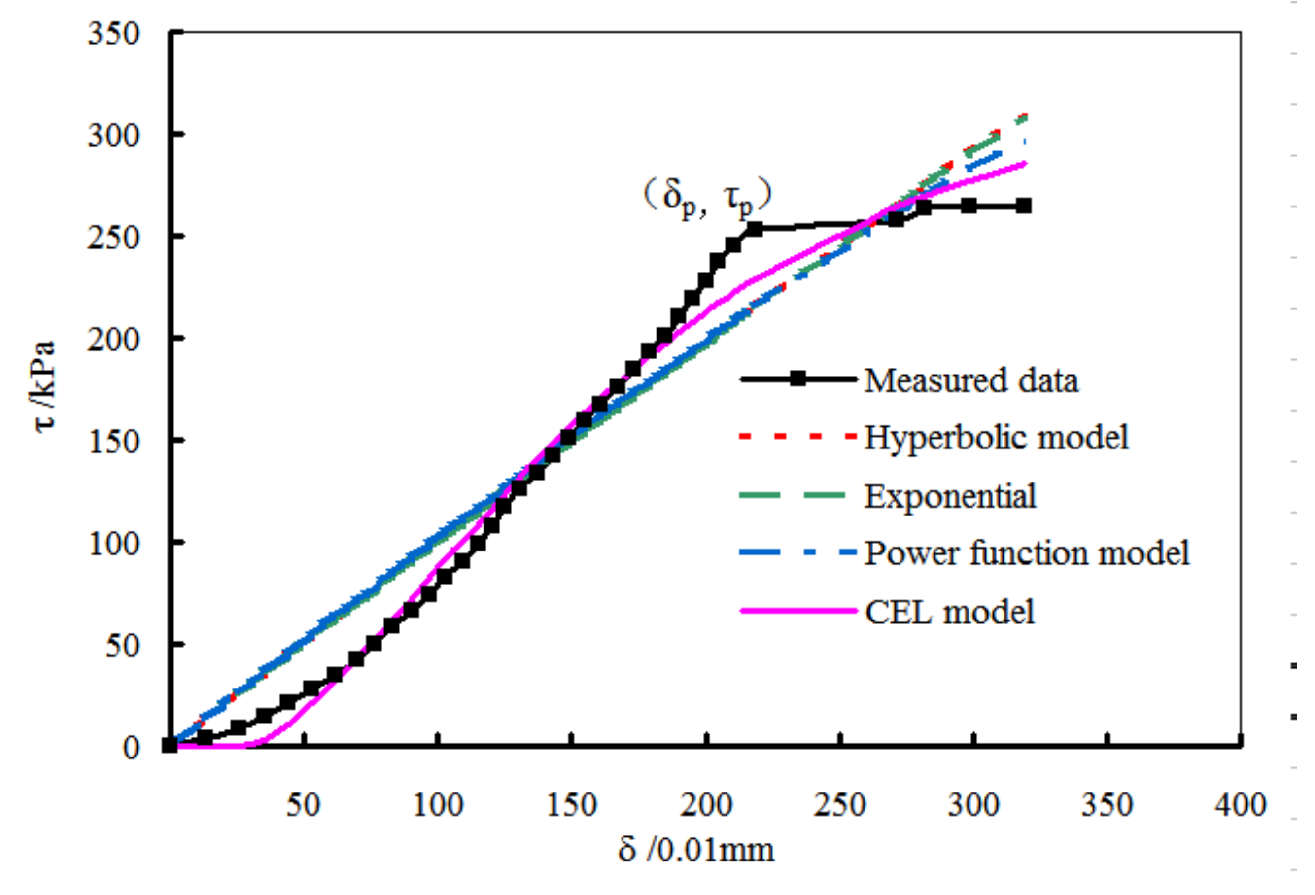
Comparisons of hyperbolic, exponential and power function models and the above CEL model are carried out based on the experimental results of two cases with 0.09 mol/L H₂SO₄ erosion under vertical pressures of 300 kPa and 400 kPa, respectively. The results are shown in Figure 11 and Figure 12.

As can be seen, the curves of conventional models are well banded which are above the measured curve before the inflection point and below the measured curve after the inflection curve. In contrast, the fitting effect of CEL model is obviously better than that of the other conventional models. It is basically consistent with the measure curve in the S-shaped range and converges faster and closer to τ_p than the other models in the failure stage. However, at the initial stage, the CEL curve is slightly lower than the measure curve, while in the failure stage, the difference between the CEL curve and the measured curve is relatively evident.

5. Conclusions

This study analyses the experimental data of τ-δ and σ-δ constitutive relationships of Nmcs, and examines its characteristics under various conditions. Two mathematical models, i.e., REP (reinforced exponential and power function) and CEL (coupled exponential and linear) models, are proposed to overcome the shortcomings of conventional models in the modeling of hardening, modified falling, S-type falling, and strong softening stress–strain behaviors. Some key findings are summarized as below:

• The τ-δ curves with varying cement mixing ratio, Nm mixing ratio and acid erosion concentrations exhibit different behaviors. For example, hardening behavior occurs with low cement mixing ratio; falling behavior takes place after adding Nm and S-type happens with acid erosion environment.
• The proposed REP model is able to satisfy the mathematical characteristics of the stress–strain curves with hardening and modified falling behaviors as well as strong softening behavior. Compared with conventional hyperbolic model, exponential and power function models which easily produce double-“X” discrepancies, the REP model has an evidently higher fitting accuracy in modeling both hardening and modified falling curves. In the modeling of strong softening behavior, the REP model also performs the best. In addition, by introducing an acid erosion factor, the REP model can be further expressed as a sulfuric acid erosion damage model which includes only three typical parameters, i.e., sulfuric acid concentration, cohesion of silty clay, and internal friction angle.
• In the modeling of S-type stress–strain behavior, the conventional models are unable to simulate the characteristic with inflection point and produce even bigger “X” discrepancy than that in the modeling of hardening and falling behavior. In contrast, the proposed CEL model performs much better especially in modeling the range around the inflection point at the early stage.

The applicability of the proposed method of this study in practice mainly include two parts. As introduced in the study, the seashore soft soil discussed herein was collected from coastal areas in Shaoxing, Zhejiang Province, China. Thus, for the regions with similar seashore soft soil, e.g., the Yangtze river delta region of China, the reported methods in this study could be used directly. On the other hand, for regions with different seashore soft soil (i.e., the soil specific gravity, LL, PL vary a lot), the proposed expressions are still applicable if the specific soil stress–strain behavior was exhibited, e.g., strong softening behavior. However, it should be noted that, for the latter scenario, the corresponding calculation parameters should be re-calibrated through laboratory tests.

References

- Al-Bared, M.A.M.; Marto, A.; Latifi, N.; Horpibulsuk, S. Sustainable improvement of marine clay using recycled blended tiles. Geotech. Geol. Eng. 2018, 36, 3135–3147. [Google Scholar] [CrossRef]
- Yao, K.; An, D.L.; Wang, W.; Li, N.; Zhang, C.; Zhou, A.Z. Effect of nano-MgO on mechanical performance of cement stabilized silty clay. Mar. Georesour. Geotechnol. 2019, 37, 250–255. [Google Scholar] [CrossRef]
- Yao, K.; Wang, W.; Li, N.; Zhang, C.; Wang, L. Investigation on strength and microstructure characteristics of nano-MgO admixed with cemented soft soil. Constr. Build. Mater. 2019, 206, 160–168. [Google Scholar] [CrossRef]
- Puppala, A.J.; Griffin, J.A.; Hoyos, L.R.; Chomtid, S. Studies on sulfate-resistant cement stabilization methods to address sulfate-induced soil heave. J. Geotech. Geoenviron. Eng. 2004, 130, 391–402. [Google Scholar] [CrossRef]
- Subramaniam, P.; Banerjee, S. Factors affecting shear modulus degradation of cement treated clay. Soil Dyn. Earthq. Eng. 2014, 65, 181–188. [Google Scholar] [CrossRef]
- Xiao, H.W.; Lee, F.H.; Chin, K.G. Yielding of cement-treated marine clay. Soils Found. 2014, 54, 488–501. [Google Scholar] [CrossRef]
- Pan, Y.T.; Liu, Y.; Chen, E. Probabilistic investigation on defective jet-grouted cut-off wall with random geometric imperfections. Géotechnique 2018, 69, 420–433. [Google Scholar] [CrossRef]
- Pan, Y.T.; Liu, Y.; Lee, F.H.; Phoon, K.K. Analysis of cement-treated soil slab for deep excavation support–a rational approach. Géotechnique 2018, 69, 888–905. [Google Scholar] [CrossRef]
- Du, H.J.; Pang, S.D. Value-added utilization of marine clay as cement replacement for sustainable concrete production. J. Clean. Prod. 2018, 198, 867–873. [Google Scholar] [CrossRef]
- Park, C.G.; Yun, S.W.; Baveye, P.C.; Yu, C. Effect of Industrial By-Products on Unconfined Compressive Strength of Solidified Organic Marine Clayey Soils. Materials 2015, 8, 5098–5111. [Google Scholar] [CrossRef]
- Du, H.J.; Pang, S.D. Dispersion and stability of graphene nanoplatelet in water and its influence on cement composites. Constr. Build. Mater. 2018, 167, 403–413. [Google Scholar] [CrossRef]
- Kang, G.O.; Tsuchida, T.; Kim, Y.S. Strength and stiffness of cement-treated marine dredged clay at various curing stages. Constr. Build. Mater. 2017, 132, 71–84. [Google Scholar] [CrossRef]
- Choobbasti, A.J.; Vafaei, A.; Kutanaei, S.S. Static and cyclic triaxial behavior of cemented sand with nanosilica. J. Mater. Civ. Eng. 2018, 30, 04018269. [Google Scholar] [CrossRef]
- Choobbasti, A.J.; Kutanaei, S.S. Microstructure characteristics of cement-stabilized sandy soil using nanosilica. J. Rock Mech. Geotech. Eng. 2017, 9, 981–988. [Google Scholar] [CrossRef]
- Choobbasti, A.J.; Vafaei, A.; Kutanaei, S.S. Mechanical properties of sandy soil improved with cement and nanosilica. Open Eng. 2015, 5, 111–116. [Google Scholar] [CrossRef]
- Song, S.Q.; Jiang, L.H.; Jiang, S.H.; Yan, X.C.; Xu, N. The mechanical properties and electrochemical behavior of cement paste containing nano-MgO at different curing temperature. Constr. Build. Mater. 2018, 164, 663–671. [Google Scholar] [CrossRef]
- Wang, W.; Zhang, C.; Li, N.; Tao, F.F.; Yao, K. Characterisation of nano magnesia–cement-reinforced seashore soft soil by direct-shear test. Mar. Georesour. Geotechnol. 2019, 37, 989–998. [Google Scholar] [CrossRef]
- Wang, D.X.; Zhu, J.Y.; He, F.J. CO2 carbonation-induced improvement in strength and microstructure of reactive MgO-CaO-fly ash-solidified soils. Constr. Build. Mater. 2019, 229, 116914. [Google Scholar] [CrossRef]
- Polat, R.; Demirboğa, R.; Karagöl, F. The effect of nano-MgO on the setting time, autogenous shrinkage, microstructure and mechanical properties of high performance cement paste and mortar. Constr. Build. Mater. 2017, 156, 208–218. [Google Scholar] [CrossRef]
- Ghasabkolaei, N.; Choobbasti, A.J.; Roshan, N.; Ghasemi, S.E. Geotechnical properties of the soils modified with nanomaterials: A comprehensive review. Arch. Civ. Mech. Eng. 2017, 17, 639–650. [Google Scholar] [CrossRef]
- Kutanaei, S.S.; Choobbasti, A.J. Experimental study of combined effects of fibers and nanosilica on mechanical properties of cemented sand. J. Mater. Civ. Eng. 2016, 28, 06016001. [Google Scholar] [CrossRef]
- Kutanaei, S.S.; Choobbasti, A.J. Effects of nanosilica particles and randomly distributed fibers on the ultrasonic pulse velocity and mechanical properties of cemented sand. J. Mater. Civ. Eng. 2017, 29, 04016230. [Google Scholar] [CrossRef]
- Deb, K. A mathematical model to study the soil arching effect in stone column-supported embankment resting on soft foundation soil. Appl. Math. Model. 2010, 34, 3871–3883. [Google Scholar] [CrossRef]
- Ungureanu, N.; Biris, S.S.; Vladut, V.; Voicu, G.; Paraschiv, G. Studies on the mathematical modeling of artificial soil compaction. Acta Tech. Corviniensis Bull. Eng. 2015, 8, 85. [Google Scholar]
- Meng, R.; Yin, D.; Zhou, C.; Wu, H. Fractional description of time-dependent mechanical property evolution in materials with strain softening behavior. Appl. Math. Model. 2016, 40, 398–406. [Google Scholar] [CrossRef]
- Mei, G.X.; Chen, R.; Liu, J. New insight into developing mathematical models for predicting deformation-dependent lateral earth pressure. Int. J. Geomech. 2017, 17, 06017003. [Google Scholar] [CrossRef]
- Ahmad, J.; Noor, M.; Jais, I.; Rosli, M.; Rahman, A.; Senin, S.; Ibrahim, A.; Hadi, B. Mathematical models for stress–strain curve prediction-a review. In AIP Conference Proceedings; AIP Publishing: Melville, NY, USA, 2018; p. 020005. [Google Scholar]
- Tarasov, B.G.; Sadovskii, V.M.; Sadovskaya, O.V.; Cassidy, M.J.; Randolph, M.F. Modeling the static stress–strain state around the fan-structure in the shear rupture head. Appl. Math. Model. 2018, 57, 268–279. [Google Scholar] [CrossRef]
- Ai, Z.Y.; Gui, J.C.; Mu, J.J. 3-D time-dependent analysis of multilayered cross-anisotropic saturated soils based on the fractional viscoelastic model. Appl. Math. Model. 2019, 76, 172–192. [Google Scholar] [CrossRef]
- Cui, L.; Fall, M. Mathematical modeling of cemented tailings backfill: A review. Int. J. Min. Reclam. Environ. 2019, 33, 389–408. [Google Scholar] [CrossRef]
- Wang, J.; Zhou, D.; Zhang, Y.Q.; Cai, W. Vertical impedance of a tapered pile in inhomogeneous saturated soil described by fractional viscoelastic model. Appl. Math. Model. 2019, 75, 88–100. [Google Scholar] [CrossRef]
- Lee, K.; Chan, D.; Lam, K. Constitutive model for cement treated clay in a critical state frame work. Soils Found. 2004, 44, 69–77. [Google Scholar] [CrossRef]
- Bergado, D.; Taechakumthorn, C.; Lorenzo, G.; Abuel-Naga, H.M. Stress-deformation behavior under anisotropic drained triaxial consolidation of cement-treated soft Bangkok clay. Soils Found. 2006, 46, 629–637. [Google Scholar] [CrossRef]
- Chiu, C.F.; Zhu, W.; Zhang, C.L. Yielding and shear behavior of cement-treated dredged materials. Eng. Geol. 2009, 103, 1–12. [Google Scholar] [CrossRef]
- Tremblay, H.; Leroueil, S.; Locat, J. Mechanical improvement and vertical yield stress prediction of clayey soils from eastern Canada treated with lime or cement. Can. Geotech. J. 2001, 38, 567–579. [Google Scholar] [CrossRef]
- Du, Y.J.; Horpibulsuk, S.; Wei, M.L.; Suksiripattanapong, C.; Liu, M.D. Modeling compression behavior of cement-treated zinc-contaminated clayey soils. Soils Found. 2014, 54, 1018–1026. [Google Scholar] [CrossRef]
- Subramaniam, P.; Sreenadh, M.M.; Banerjee, S. Critical state parameters of dredged Chennai marine clay treated with low cement content. Mar. Georesour. Geotechnol. 2016, 34, 603–616. [Google Scholar] [CrossRef]
- Yu, B.W.; Du, Y.J.; Jin, F.; Liu, C.Y. Multiscale study of sodium sulfate soaking durability of low plastic clay stabilized by reactive magnesia-activated ground granulated blast-furnace slag. J. Mater. Civ. Eng. 2016, 28, 04016016. [Google Scholar] [CrossRef]
- Wang, W.; Li, Y.; Yao, K.; Li, N.; Zhou, A.Z.; Zhang, C. Strength properties of nano-MgO and cement stabilized coastal silty clay subjected to sulfuric acid attack. Mar. Georesour. Geotechnol. 2019. [Google Scholar] [CrossRef]
- Duncan, J.M.; Chang, C.Y. Nonlinear analysis of stress and strain in soils. J. Soil Mech. Found. Div. 1970, 96, 1629–1653. [Google Scholar]
- Cai, Y.Y.; Zheng, C.T.; Qi, Z.B.; Mu, K.; Yu, J. Nonlinear constitutive model of clay based on power function. J. Lanzhou Univ. Technol. 2012, 38, 126–130. [Google Scholar]
© 2020 by the authors. Licensee MDPI, Basel, Switzerland. This article is an open access article distributed under the terms and conditions of the Creative Commons Attribution (CC BY) license (http://creativecommons.org/licenses/by/4.0/).