Article

Stability Analysis of an Age-Structured SEIRS Model with Time Delay

Department of mathematics, Beijing Jiaotong University, Beijing 100044, China
*
Author to whom correspondence should be addressed.
Mathematics 2020, 8(3), 455; https://doi.org/10.3390/math8030455
Submission received: 20 February 2020 / Revised: 18 March 2020 / Accepted: 19 March 2020 / Published: 23 March 2020
(This article belongs to the Special Issue Models of Delay Differential Equations)

Abstract

:
This paper is concerned with the stability of an age-structured susceptible–exposed– infective–recovered–susceptible (SEIRS) model with time delay. Firstly, the traveling wave solution of system can be obtained by using the method of characteristic. The existence and uniqueness of the continuous traveling wave solution is investigated under some hypotheses. Moreover, the age-structured SEIRS system is reduced to the nonlinear autonomous system of delay ODE using some insignificant simplifications. It is studied that the dimensionless indexes for the existence of one disease-free equilibrium point and one endemic equilibrium point of the model. Furthermore, the local stability for the disease-free equilibrium point and the endemic equilibrium point of the infection-induced disease model is established. Finally, some numerical simulations were carried out to illustrate our theoretical results.

1. Introduction

In recent years, the study of epidemiology has been a vital problem in ecology. The research of population dynamics has developed rapidly, and many mathematical models have been used to analyze various infectious diseases. Many results have been established in the stability analysis of different epidemic models. The first susceptible–infective–recovered (SIR) epidemic model about disease transmission was established by Kermack and McKendrick in 1927 [1]. Since then, the population dynamics of infectious diseases have attracted the attention of scientists. In 2012, the field of mathematical biology was expanded, particularly in the context of the spread of infectious diseases by Fred Brauer et al. [2]. Nowadays, there are some research work devoted to study the stability of steady states of the SIR, SIRS, SEIR, etc. models [3,4,5,6,7]. It is well known, in the spread of infectious diseases, some infective individuals of population are immune after being recovered (e.g., measles, smallpox, mumps, and others). Meanwhile, some recovered individuals have no immunity (e.g., AIDS, hyperthyroidism, lupus erythematosus, and others), who will return to the susceptible population and continue to be infected. In fact, the probability of becoming infected is different among different individuals, which may depend on the type of infectious diseases and the status of individuals. Therefore, it is necessary to discuss the SEIRS model, which can more clearly describe the spread of infectious diseases in real life.
Time delay is ubiquitous and can be applied in many epidemiology related studies [8,9]. For example, measles has an incubation period of 8–13 days and the incubation period of canine madness is a few months or several years after infection. Sharma et al. [10] developed a five compartmental infection model to describe the spread of avian influenza A (H7N9) virus with two discrete time delays. In addition, Xu et al. [11] analyzed the stability of a SIRS model with time delay. Similarly, Shu [12] and De la Sena [13] discussed the stability of the SEIR epidemic models with distributed delay respectively. Actually, many authors, such as Cooke [14], Gao [15] and Wang [16], have studied various SEIRS models with time delay.
Besides, age structure is also an important consideration in infectious diseases modeling such as rubella, poliomyelitis, and pertussis, which are transmitted only among children, and venereal diseases, which are transmitted only among adults. Besides, tuberculosis virus carriers in the early incubation period have a higher risk of becoming infective individuals than ones in the late incubation period [17]. Age-structured models have been applied in the epidemic dynamics for decades. In 1986, the dynamics of structured populations was discussed by Metz et al. [18]. Then, the mathematical theory of the age-structured population dynamics was proposed by Iannelli [19]. Afterwards, more and more epidemic models with age structure were studied in [20,21,22,23,24,25,26,27,28]. Recently, a new age-structured malaria model incorporating the age of latent period and the age of prevention period was formulated by Guo et al. [29]. A new SIRS epidemic model with relapse and infection age on a scale-free network was introduced Huo et al. [30]. However, as far as we can tell, there have been no results on an age-structured SEIRS model with time delay.
The main aim of this paper is to study the stability of an age-structured SEIRS model with time delay. The well-known method of characteristics [25,26,27,28] for first-order hyperbolic equations is used to solve this epidemic model. The explicit traveling wave solution is calculated at the preceding moment of time and is described in integral form. Under some hypotheses, the existence and uniqueness of the continuous traveling wave solution of the age-structured SEIRS model is investigated. Moreover, an age-structured SEIRS model with time delay is reduced to the nonlinear ordinary differential equation under some insignificant simplifications. After that, the dimensionless indexes are derived for the existence of the disease-free equilibrium point and the endemic equilibrium point. The local asymptotic stability of the disease-free equilibrium point is studied. By using Hurwitz’s criterion and Descartes’ rule of signs, the local asymptotic stability of the endemic equilibrium point of system is obtained.
The rest of the paper is organized as follows. In Section 2, an age-structured SEIRS model with time delay is proposed. In Section 3, the traveling wave solution is obtained and some sufficient conditions are established to guarantee the existence and uniqueness of the solution. In Section 4, the stability and Hopf bifurcation analysis of the proposed model are discussed. In Section 5, numerical simulations are provided to illustrate the effectiveness of our main results. Finally, some conclusions are given in Section 6.

2. An Age-Structured SEIRS Model with Time Delay

Motivated by the referred works [28], we discuss two age stages of each subpopulation of an age-structured SEIRS model with time delay in this paper, which include immature stage and mature stage. In the immature stage, individuals can be born, grow up, die, or survive until the maximum age a 1 , but, in this case, the individuals are not proliferate until the maximum age a 1 . The age a 1 is considered to be the maximum age in the immature stage and it is also considered to be the initial age in the mature stage. In the mature stage, individuals have reached maturity ( a > a 1 ) and can grow up, proliferate, die, or survive to the maximum age A. Here, we consider susceptible, exposed, infective, and recovered individuals of two age stages in an age-structured SEIRS model. Let S ( a , t ) , E ( a , t ) , I ( a , t ) , and R ( a , t ) be the distribution densities of susceptible, exposed, infective ,and recovered individuals of age x at time t, and they take place in the domain Ω = ( a , t ) : 0 a A , 0 t T . The integrals N s ( t ) = 0 A S ( a , t ) d a , N e ( t ) = 0 A E ( a , t ) d a , N i ( t ) = 0 A I ( a , t ) d a , and N r ( t ) = 0 A R ( a , t ) d a are considered as the number of susceptible, exposed, infective and recovered individuals, respectively. The total population N ( t ) is: N ( t ) = N s ( t ) + N e ( t ) + N i ( t ) + N r ( t ) . What needs to be added is that S ( a , t ) , E ( a , t ) , I ( a , t ) , and R ( a , t ) should belong to L 1 ( Ω ) because we assume that the initial total population is limited. Then, the following differential equations with time delay are
S t + S a = α ^ 1 ( a , t ) + σ θ ^ 1 ( a , t ) S ( a , t ) γ 1 ( a , t τ ) 0 A β ( a , a , t τ ) I ( a , t τ ) d a S ( a , t ) + ρ ( a , t ) R ( a , t ) , ( a , t ) Ω , E t + E a = α ^ 2 ( a , t ) + σ θ ^ 2 ( a , t ) E ( a , t ) + γ 1 ( a , t τ ) 0 A β ( a , a , t τ ) I ( a , t τ ) d a S ( a , t ) γ 2 ( a , t ) E ( a , t ) , ( a , t ) Ω , I t + I a = α ^ 3 ( a , t ) + σ θ ^ 3 ( a , t ) I ( a , t ) + γ 2 ( a , t ) E ( a , t ) γ 3 ( a , t ) I ( a , t ) , ( a , t ) Ω , R t + R a = α ^ 4 ( a , t ) + σ θ ^ 4 ( a , t ) R ( a , t ) + γ 3 ( a , t ) I ( a , t ) ρ ( a , t ) R ( a , t ) , ( a , t ) Ω ,
with initial conditions
S ( a , 0 ) = S 0 ( a ) , a [ 0 , A ] , E ( a , 0 ) = E 0 ( a ) , a [ 0 , A ] , I ( a , t ) = I 0 ( a , t ) , a [ 0 , A ] , t [ τ , 0 ] , R ( a , 0 ) = 0 , x [ 0 , A ] ,
and boundary conditions
S ( 0 , t ) = a 1 A ( μ 1 θ 1 ( a , t ) S ( a , t ) + μ 2 θ 2 ( a , t ) 1 p ( a , t ) E ( a , t ) + μ 3 θ 3 ( a , t ) 1 q ( a , t ) I ( a , t ) + μ 4 θ 4 ( a , t ) R ( a , t ) ) d a , t ( 0 , T ) , E ( 0 , t ) = μ 2 a 1 A p ( a , t ) θ 2 ( a , t ) E ( a , t ) d a , t ( 0 , T ) , I ( 0 , t ) = μ 3 a 1 A q ( a , t ) θ 3 ( a , t ) I ( a , t ) d a , t ( 0 , T ) , R ( 0 , t ) = 0 , t ( 0 , T ) ,
where θ ^ i ( a , t ) ( i = 1 , 2 , 3 , 4 ) denote fertility rates of females of each subpopulation of age a; θ ^ i ( a , t ) = θ i ( a , t ) , if a a 1 , A ; θ ^ i ( a , t ) = 0 , if a a 1 , A ; α ^ i ( a , t ) are natural death rates of each subpopulation of age a; σ is the provided parameter: σ = 1 if the individuals die when they produce and σ = 0 if the individuals continue to survive when they produce; γ 1 ( a , t ) is a transmission coefficient which describes the varying probability of infectiousness and it is related to a great many social, environmental, and epidemiological factors; β ( a , a , t ) is the contact rate between infected population (age a ) and susceptible population (age a) per unit time; τ ( τ > 0 ) is a fixed incubation period of infection; γ 2 ( a , t ) is the conversion rate from exposed population to infected population of age a; γ 3 ( a , t ) is the recovery rate of age a; ρ ( a , t ) is the conversion rate from recovered population losing immunity to the susceptible population of age a; μ i ( i = 1 , 2 , 3 , 4 ) are reproductive rates of each subpopulation in the proliferating stage; p ( a , t ) is part of exposed individuals which procreate new exposed individuals of age a; and, similarly, q ( a , t ) is part of infective individuals which procreate new infective individuals of age a.

3. Traveling Wave Solution

In this section, we mainly use the method of characteristics [2,18,25,26,27,28] for first-order hyperbolic partial differential equations (Equation (1)). Then, the system in Equation (1) is reduced to nonlinear delayed integro-differential equations along the characteristics curve a t = c o n s t a n t [25,26]. Let u = a t , the following system with time delay is obtained:
S t = α ^ 1 ( u + t , t ) + σ θ ^ 1 ( u + t , t ) S ( u + t , t ) γ 1 ( u + t , t τ ) 0 A β ( a , a , t τ ) I ( a , t τ ) d a × S ( u + t , t ) + ρ ( u + t , t ) R ( u + t , t ) , E t = α ^ 2 ( u + t , t ) + σ θ ^ 2 ( u + t , t ) E ( u + t , t ) + γ 1 ( u + t , t τ ) 0 A β ( a , a , t τ ) I ( a , t τ ) d a × S ( u + t , t ) γ 2 ( u + t , t ) E ( u + t , t ) , I t = α ^ 3 ( u + t , t ) + σ θ ^ 3 ( u + t , t ) I ( u + t , t ) + γ 2 ( u + t , t ) E ( u + t , t ) γ 3 ( u + t , t ) I ( u + t , t ) , R t = α ^ 4 ( u + t , t ) + σ θ ^ 4 ( u + t , t ) R ( u + t , t ) + γ 3 ( u + t , t ) I ( u + t , t ) ρ ( u + t , t ) R ( u + t , t ) ,
with initial functions
S ( u , 0 ) = S 0 ( u ) , E ( u , 0 ) = E 0 ( u ) , I ( u + t , t ) = I 0 ( u + t , t ) , t [ τ , 0 ] , R ( u , 0 ) = R 0 ( u ) = 0 .
In general, we divide time interval [ 0 , T ] into K intervals [ t k 1 , t k ] , where k = 1 , , K , t 0 = 0 , t K = T , t k = k A . Then, Ω can be grouped into two sets:
Ω k ( 1 ) = ( a , t ) | t [ ( k 1 ) A , ( a + ( k 1 ) A ) ] , a [ 0 , A ] ,
Ω k ( 2 ) = ( a , t ) | t [ ( a + ( k 1 ) A ) , k A ] , a [ 0 , A ] ,
Ω = k = 1 K ( Ω k ( 1 ) Ω k ( 2 ) ) .
We also need to define an auxiliary set for k = 1 , , K :
Ω ¯ ( k ) = [ u n ( k ) , u n + 1 ( k ) ] u n ( k ) = n a 1 + ( k 1 ) A , n = 1 , , N 1 , u N ( k ) = k A ,
where N = [ A a 1 ] + 1 , i f A a 1 [ A a 1 ] > 0 ; N = A a 1 , i f A a 1 [ A a 1 ] > 0 . [ x ] denotes a whole part of real number x. The following hypotheses are given:
( H 1 ) : S 0 ( a ) , E 0 ( a ) and I 0 ( a , 0 ) are non-negative and continuous when a [ 0 , A ] ; when a A 0 , S 0 ( A ) = 0 , E 0 ( A ) = 0 and I 0 ( A , 0 ) = 0 .
( H 2 ) : α ^ i ( a , t ) , θ i ( a , t ) , γ i ( a , t ) , β ( a , t ) , ρ ( a , t ) , p ( a , t ) , q ( a , t ) C ( Ω ) .
( H 3 ) : α ^ i ( a , t ) > 0 , θ i ( a , t ) 0 , γ i ( a , t ) > 0 , β ( a , t ) 0 . In addition, 0 < a 1 A θ i ( a , t ) d a 1 , 0 < 0 A β ( a , t ) d x 1 , 0 ρ ( a , t ) 1 , 0 p ( a , t ) 1 , 0 q ( a , t ) 1 .
( H 4 ) : zero-order compatibility conditions are
S 0 ( 0 ) = a 1 A ( μ 1 θ 1 ( a , 0 ) S 0 ( a ) + μ 2 θ 2 ( a , 0 ) 1 p ( a , 0 ) E 0 ( a ) + μ 3 θ 3 ( a , 0 ) 1 q ( a , 0 ) I 0 ( a , 0 ) ) d a , E 0 ( 0 ) = μ 2 a 1 A θ 2 ( a , 0 ) p ( a , 0 ) E 0 ( a ) d a , I 0 ( 0 , 0 ) = μ 3 a 1 A θ 3 ( a , 0 ) q ( a , 0 ) I 0 ( a , 0 ) d a , R 0 ( 0 ) = 0 .
For convenience, we assume Hypotheses ( H 1 ) ( H 4 ) are satisfied.
Then, we solve the system in Equation (4) by using the well-known steps method [8,9]. For the first step h = 1 , i.e., for the first time interval t [ 0 , τ ] , the solution to the initial value problem in Equation (4) can be obtained according to the known values of function I ( x , t τ ) . Repeating the pervious step for h = 2 , 3 , 4 , , H , for the time interval t [ ( h 1 ) τ , h τ ] , we can obtain the solution to the initial value problem in Equation (4) for the whole time interval t [ 0 , T ] :
S 1 ( u , t ) = S 0 ( u ) W 1 ( u , 0 , t , τ ) + 0 t W 1 ( u , ϕ , t , τ ) ρ ( u + ϕ , ϕ ) R ( u + ϕ , ϕ ) d ϕ , t [ 0 , τ ] , S h ( u , t ) = S h 1 ( u ) W 1 ( u , ( h 1 ) τ , t , τ ) + ( h 1 ) τ t W 1 ( u , ϕ , t , τ ) ρ ( u + ϕ , ϕ ) R ( u + ϕ , ϕ ) d ϕ = S 0 ( u ) W 1 ( v , 0 , t , τ ) + 0 t W 1 ( u , ϕ , t , τ ) ρ ( v + ϕ , ϕ ) R ( u + ϕ , ϕ ) d ϕ , t [ ( h 1 ) τ , h τ ] , W 1 ( u , t 0 , t , τ ) = e x p ( t 0 t ( α 1 ( u + ϕ , ϕ ) + γ 1 ( u + ϕ , ϕ τ ) D ( u + ϕ , ϕ τ ) ) d ϕ ) ,
E 1 ( u , t ) = E 0 ( u ) W 2 ( u , 0 , t ) + 0 t W 2 ( u , ϕ , t ) γ 1 ( u + ϕ , ϕ τ ) S ( u + ϕ , ϕ ) D ( u + ϕ , ϕ τ ) d ϕ , t [ 0 , τ ] , E h ( u , t ) = E h 1 ( u ) W 2 ( u , ( h 1 ) τ , t ) + ( h 1 ) τ t W 2 ( u , ϕ , t ) γ 1 ( u + ϕ , ϕ τ ) S ( u + ϕ , ϕ ) × D ( u + ϕ , ϕ τ ) d ϕ = E 0 ( u ) W 2 ( u , 0 , t ) + 0 t W 2 ( u , ϕ , t ) γ 1 ( u + ϕ , ϕ τ ) × S ( u + ϕ , ϕ ) D ( u + ϕ , ϕ τ ) d ϕ , t [ ( h 1 ) τ , h τ ] , W 2 ( u , t 0 , t ) = e x p ( t 0 t α 2 ( u + ϕ , ϕ ) + γ 2 ( u + ϕ , ϕ ) d ϕ ) ,
I 1 ( u , t ) = I 0 ( u , 0 ) W 3 ( u , 0 , t ) + 0 t W 3 ( u , ϕ , t ) γ 2 ( u + ϕ , ϕ τ ) E ( u + ϕ , ϕ ) d ϕ , t [ 0 , τ ] , I h ( u , t ) = I h 1 ( u , ( h 1 ) τ ) W 3 ( u , ( h 1 ) τ , t ) + ( h 1 ) τ t W 3 ( u , ϕ , t ) γ 2 ( u + ϕ , ϕ τ ) × E ( u + ϕ , ϕ ) d ϕ = I 0 ( u , 0 ) W 3 ( u , 0 , t ) + 0 t W 3 ( u , ϕ , t ) γ 2 ( u + ϕ , ϕ τ ) × E ( u + ϕ , ϕ ) d ϕ , t [ ( h 1 ) τ , h τ ] , W 3 ( u , t 0 , t ) = e x p ( t 0 t ( α 3 ( u + ϕ , ϕ ) + γ 3 ( u + ϕ , ϕ ) ) d ϕ ) ,
R 1 ( u , t ) = 0 t W 4 ( u , ϕ , t ) γ 3 ( u + ϕ , ϕ τ ) I ( u + ϕ , ϕ ) d ϕ , t [ 0 , τ ] R h ( u , t ) = R h 1 ( u , ( h 1 ) τ ) W 4 ( u , ( h 1 ) τ ) , t ) + ( h 1 ) τ t W 4 ( u , ϕ , t ) γ 3 ( u + ϕ , ϕ τ ) × I ( u + ϕ , ϕ ) d ϕ = 0 t W 4 ( u , ϕ , t ) γ 3 ( u + ϕ , ϕ τ ) I ( u + ϕ , ϕ ) d ϕ , t [ ( h 1 ) τ , h τ ] , W 4 ( u , t 0 , t ) = e x p ( t 0 t α 4 ( u + ϕ , ϕ ) + ρ ( u + ϕ , ϕ ) d ϕ ) ,
where α i ( a , t ) = α ^ i ( a , t ) + σ θ ^ i ( a , t ) , i = 1 , 2 , 3 , 4 , D ( u + ϕ , ϕ τ ) = 0 A β ( u + ϕ , η , ϕ τ ) I ( η , ϕ τ ) d η .
The exact solution to Equations (11)–(14) of the system in Equation (4) can be expressed in terms of the original variables. Let k = 1 and u = a t ; we have the solution of the system in Equation (1) in the sets Ω k ( 1 ) and Ω k ( 2 ) . Repeating this process for k = 2 , 3 , K , the form of explicit traveling wave solution, i.e., numerical solution of the system in Equation (1), can be obtained in all domains Ω k ( 1 ) and Ω k ( 2 ) for the values of k = 1 , , K :
( S ( a , t ) , E ( a , t ) , I ( a , t ) , R ( a , t ) ) = S h ( k 1 ) ( u , t ) = S h ( k 1 ) ( a t , t ) , E h ( k 1 ) ( u , t ) = E h ( k 1 ) ( a t , t ) , I h ( k 1 ) ( u , t ) = I h ( k 1 ) ( a t , t ) , R h ( k 1 ) ( u , t ) = R h ( k 1 ) ( a t , t ) , i f ( a , t ) Ω k ( 1 ) , S h ( k ) ( u , t ) = S h ( k ) ( a t , t ) , E h ( k ) ( u , t ) = E h ( k ) ( a t , t ) , I h ( k ) ( u , t ) = I h ( k ) ( a t , t ) , R h ( k ) ( u , t ) = R h ( k ) ( a t , t ) , i f ( a , t ) Ω k ( 2 ) ,
S ( 0 ) ( u , t ) = S 0 ( u ) W 1 ( u , 0 , t , τ ) + 0 t W 1 ( u , ϕ , t , τ ) ρ ( u + ϕ , ϕ ) R ( 0 ) ( u + ϕ , ϕ ) d ϕ , S ( k ) ( u , t ) = F ( k ) ( u ) W 1 ( u , u , t , τ ) + u t W 1 ( u , ϕ , t , τ ) ρ ( u + ϕ , ϕ ) R ( k ) ( u + ϕ , ϕ ) d ϕ ,
E ( 0 ) ( u , t ) = E 0 ( u ) W 2 ( u , 0 , t ) + 0 t W 2 ( u , ϕ , t ) γ 1 ( u + ϕ , ϕ τ ) S ( 0 ) ( u + ϕ , ϕ ) D ( u + ϕ , ϕ τ ) d ϕ , E ( k ) ( u , t ) = G ( k ) ( u ) W 2 ( u , u , t ) + u t W 2 ( u , ϕ , t ) γ 1 ( u + ϕ , ϕ τ ) S ( k ) ( u + ϕ , ϕ ) D ( u + ϕ , ϕ τ ) d ϕ ,
I ( 0 ) ( u , t ) = I 0 ( u , 0 ) W 3 ( u , 0 , t ) + 0 t W 3 ( u , ϕ , t ) γ 2 ( u + ϕ , ϕ τ ) E ( 0 ) ( u + ϕ , ϕ ) d ϕ , I ( k ) ( u , t ) = Q ( k ) ( u ) W 3 ( u , u , t ) + u t W 3 ( u , ϕ , t ) γ 2 ( u + ϕ , ϕ τ ) E ( k ) ( u + ϕ , ϕ ) d ϕ ,
R ( 0 ) ( u , t ) = 0 t W 4 ( u , ϕ , t ) γ 3 ( u + ϕ , ϕ τ ) I ( 0 ) ( u + ϕ , ϕ ) d ϕ , R ( k ) ( u , t ) = u t W 4 ( u , ϕ , t ) γ 3 ( u + ϕ , ϕ τ ) I ( k ) ( u + ϕ , ϕ ) d ϕ ,
where W 1 ( u , t 0 , t , τ ) , W 2 ( u , t 0 , t ) , W 3 ( u , t 0 , t ) , and W 4 ( u , t 0 , t ) are shown in Equations (11)–(14), respectively. F ( k ) ( u ) , G ( k ) ( u ) , and Q ( k ) ( u ) are given by defining functions F n ( k ) ( u ) , G n ( k ) ( u ) , Q n ( k ) ( u ) , S n ( k ) ( u ) , E n ( k ) ( u ) , I n ( k ) ( u ) , and R n ( k ) ( u ) , k = 1 , , K :
( F ( k ) ( u ) ) , G ( k ) ( u ) , Q ( k ) ( u ) ) = ( F n ( k ) ( u ) ) , G n ( k ) ( u ) , Q n ( k ) ( u ) ) , u [ u n ( k ) , u n 1 ( k ) ] , n = 1 , , N τ ,
thus we have
S n ( k ) ( u , t ) = F n ( k ) ( u ) W 1 ( u , u , t , τ ) + u t W 1 ( u , ϕ , t , τ ) ρ ( u + ϕ , ϕ ) R n ( k ) ( u + ϕ , ϕ ) d ϕ , E n ( k ) ( u , t ) = G n ( k ) ( u ) W 2 ( u , u , t ) + u t W 2 ( u , ϕ , t ) γ 1 ( u + ϕ , ϕ τ ) S n ( k ) ( u + ϕ , ϕ ) D ( u + ϕ , ϕ τ ) d ϕ , I n ( k ) ( u , t ) = Q n ( k ) ( u ) W 3 ( u , u , t ) + u t W 3 ( u , ϕ , t ) γ 2 ( u + ϕ , ϕ τ ) E n ( k ) ( u + ϕ , ϕ ) d ϕ , R n ( k ) ( u , t ) = u t W 4 ( u , ϕ , t ) γ 3 ( u + ϕ , ϕ τ ) I n ( k ) ( u + ϕ , ϕ ) d ϕ ,
where n = 1 , , N τ 1 and functions F n ( k ) ( u ) , G n ( k ) ( u ) , and Q n ( k ) ( u ) can be defined according to the recurrent algorithm as follows:
F 1 ( k ) ( v ) = a 1 + v A + v [ μ 1 θ 1 ( u v , v ) S ( k 1 ) ( u , v ) + μ 2 θ 2 ( u v , v ) 1 p ( u v , v ) E ( k 1 ) ( u , v ) + μ 3 θ 3 ( u v , v ) 1 q ( u v , v ) I ( k 1 ) ( u , v ) + μ 4 θ 4 ( u v , v ) R ( k 1 ) ( u , v ) ] d u , v [ u 1 ( k ) , u 0 ( k ) ] , G 1 ( k ) ( v ) = μ 2 a 1 + v A + v p ( u v , v ) θ 2 ( u v , u ) E ( k 1 ) ( u , v ) d u , v [ u 1 ( k ) , u 0 ( k ) ] , Q 1 ( k ) ( v ) = μ 3 a 1 + v A + v q ( u v , v ) θ 3 ( u v , u ) I ( k 1 ) ( u , v ) d u , v [ u 1 ( k ) , u 0 ( k ) ] , F 2 ( k ) ( v ) = a 1 + v u 0 ( k ) [ μ 1 θ 1 ( u v , v ) S ( k ) ( u , v ) + μ 2 θ 2 ( u v , v ) 1 p ( u v , v ) E ( k ) ( u , v ) + μ 3 θ 3 ( u v , v ) 1 q ( u v , v ) I ( k ) ( u , v ) + μ 4 θ 4 ( u v , v ) R ( k ) ( u , v ) ] d u + u 0 ( k ) A + v [ μ 1 θ 1 ( u v , v ) S ( k 1 ) ( u , v ) + μ 2 θ 2 ( u v , v ) 1 p ( u v , v ) × E ( k 1 ) ( u , v ) + μ 3 θ 3 ( u v , v ) 1 q ( u v , v ) I ( k 1 ) ( u , v ) + μ 4 θ 4 ( u v , v ) × R ( k 1 ) ( u , v ) ] d u , v [ u 2 ( k ) , u 1 ( k ) ] , G 2 ( k ) ( v ) = μ 2 a 1 + v u 0 ( k ) p ( u v , v ) θ 2 ( u v , u ) E ( k ) ( u , v ) d u + μ 2 u 0 ( k ) A + v p ( u v , v ) × θ 2 ( u v , u ) E ( k 1 ) ( u , v ) d u , v [ u 2 ( k ) , u 1 ( k ) ] , Q 2 ( k ) ( v ) = μ 3 a 1 + v u 0 ( k ) q ( u v , v ) θ 3 ( u v , u ) I ( k ) ( u , v ) d u + μ 3 u 0 ( k ) A + v q ( u v , v ) × θ 3 ( u v , u ) I ( k 1 ) ( u , v ) d u , v [ u 2 ( k ) , u 1 ( k ) ] , F n ( k ) ( v ) = a 1 + v u n 2 ( k ) [ μ 1 θ 1 ( u v , v ) S ( k ) ( u , v ) + μ 2 θ 2 ( u v , v ) 1 p ( u v , v ) E ( k ) ( u , v ) + μ 3 θ 3 ( u v , v ) 1 q ( u v , v ) I ( k ) ( u , v ) + μ 4 θ 4 ( u v , v ) R ( k ) ( u , v ) ] d u + i = 0 n 3 u i + 1 ( k ) u i ( k ) [ μ 1 θ 1 ( u v , v ) S i + 1 ( k ) ( u , v ) + μ 2 θ 2 ( u v , v ) 1 p ( u v , v ) × E i + 1 ( k ) ( u , v ) + μ 3 θ 3 ( u v , v ) 1 q ( u v , v ) I i + 1 ( k ) ( u , v ) + μ 4 θ 4 ( u v , v ) + R i + 1 ( k ) ( u , v ) ] d u + u 0 ( k ) A + v [ μ 1 θ 1 ( u v , v ) S ( k 1 ) ( u , v ) + μ 2 θ 2 ( u v , v ) × 1 p ( u v , v ) E ( k 1 ) ( u , v ) + μ 3 θ 3 ( u v , v ) 1 q ( u v , v ) I ( k 1 ) ( u , v ) + μ 4 θ 4 ( u v , v ) R ( k 1 ) ( u , v ) ] d u , v [ u n ( k ) , u n 1 ( k ) ] , n = 3 , , N τ , G n ( k ) ( v ) = μ 2 a 1 + v u n 2 ( k ) p ( u v , v ) θ 2 ( u v , u ) E n 1 ( k ) ( u , v ) d u + μ 2 i = 0 n 3 u i + 1 ( k ) u i ( k ) p ( u v , v ) × θ 2 ( u v , u ) E i + 1 ( k ) ( u , v ) d u + μ 2 u 0 ( k ) A + v p ( u v , v ) θ 2 ( u v , u ) E ( k 1 ) ( u , v ) d u , v [ u n ( k ) , u n 1 ( k ) ] , n = 3 , , N τ ,
Q n ( k ) ( v ) = μ 3 a 1 + v u n 2 ( k ) q ( u v , v ) θ 3 ( u v , u ) I n 1 ( k ) ( u , v ) d u + μ 3 i = 0 n 3 u i + 1 ( k ) u i ( k ) q ( u v , v ) × θ 3 ( u v , u ) I i + 1 ( k ) ( u , v ) d u + μ 3 u 0 ( k ) A + v q ( u v , v ) θ 3 ( u v , u ) I ( k 1 ) ( u , v ) d u , v [ u n ( k ) , u n 1 ( k ) ] , n = 3 , , N τ , F 1 ( k ) ( u ) = a 1 A [ μ 1 θ 1 ( v , u ) S ( k 1 ) ( v , u ) + μ 2 θ 2 ( v , u ) 1 p ( v , u ) E ( k 1 ) ( v , u ) + μ 3 θ 3 ( v , u ) 1 q ( v , u ) I ( k 1 ) ( v , u ) + μ 4 θ 4 ( v , u ) R ( k 1 ) ( v , u ) ] d v , G ( k ) ( u ) = μ 2 a 1 A p ( v , u ) θ 2 ( v , u ) E ( k 1 ) ( v , u ) d v , Q ( k ) ( u ) = μ 3 a 1 A q ( v , u ) θ 3 ( v , u ) I ( k 1 ) ( v , u ) d v .
Theorem 1.
If Assumptions ( H 1 ) ( H 4 ) are satisfied, there exists a unique continuous traveling wave solution to Equations (15)–(19) of the system in Equation (1).
Proof. 
By analogy with [28], if S 0 ( a ) , E 0 ( a ) , I 0 ( a , 0 ) , and R 0 ( a ) satisfy compatibility conditions (i.e., Hypothesis H 4 ), then two parts of the traveling wave in Equation (15) can be combined continuously. If the parameters of the system in Equation (1) fulfill Hypotheses ( H 1 ) ( H 3 ) , there exists a unique continuous traveling wave solution to Equations (15)–(19) of the system in Equation (1). The method is very similar, thus we omit it. □

4. Stability Analysis of System

Consider the nonlinear autonomous system in Equation (1) where the following parameters are constants: θ i ( a , t ) = θ i 0 ( i = 1 , 2 , 3 , 4 ) , α i ( a , t ) = α i 0 = α i + σ θ i 0 ( i = 1 , 2 , 3 , 4 ) , γ 1 ( a , t ) = γ 10 , γ 2 ( a , t ) = γ 20 , γ 3 ( a , t ) = γ 30 , β ( a , a , t ) = β 0 , p ( a , t ) = p 0 , q ( a , t ) = q 0 , and ρ ( a , t ) = ρ 0 , where α i 0 , θ i 0 , γ i 0 , β 0 , p 0 , q 0 , and ρ 0 are positive constants. In this paper, a partial differential equation (Equation (1)) with the initial-boundary values in Equations (2) and (3) reduced to a nonlinear ordinary differential equation. Take the maturity age a 1 0 , which is not an essential simplification. Integrating Equation (1) in regard to age a from 0 to A, and using the real conditions S ( A , t ) = 0 , E ( A , t ) = 0 , I ( A , t ) = 0 and R ( A , t ) = 0 , the initial value problem of the nonlinear ordinary differential equation autonomous system that describes the population dynamics of the number of population N s ( t ) , N e ( t ) , N i ( t ) , and N r ( t ) is:
N s ( t ) = ( α 10 μ 1 θ 10 ) N s ( t ) γ 10 β 0 N s ( t ) N i ( t τ ) + μ 2 θ 20 ( 1 p 0 ) N e ( t ) + μ 3 θ 30 ( 1 q 0 ) N i ( t ) + ( μ 4 θ 40 + ρ 0 ) N r ( t ) , N e ( t ) = ( α 20 + γ 20 μ 2 θ 20 p 0 ) N e ( t ) + γ 10 β 0 N s ( t ) N i ( t τ ) , N i ( t ) = ( α 30 + γ 30 μ 3 θ 30 q 0 ) N i ( t ) + γ 20 N e ( t ) , N r ( t ) = ( α 40 + ρ 0 ) N r ( t ) + γ 30 N i ( t ) ,
with initial functions
N s ( 0 ) = 0 A S 0 ( a ) d a , N e ( t ) = 0 A E 0 ( a , t ) d a , t [ τ , 0 ] , N i ( 0 ) = 0 A I 0 ( a ) d a , N r ( 0 ) = 0 .
The basic reproduction number [31] is defined as
R 0 = N γ 20 γ 10 β 0 ( α 20 + γ 20 μ 2 θ 20 p 0 ) ( α 30 + γ 30 μ 3 θ 30 q 0 ) .
According to the analysis of [28], if R 0 > 1 , it can lead to the outbreak of infectious diseases. Hence, the following theorem is obtained.
Theorem 2.
If γ 10 = 0 , the system in Equation (20) has only a disease-free equilibrium point H 0 = ( 0 , 0, 0, 0 ) ; if R 0 > 1 and the parameters of the system in Equation (20) satisfy R 1 > 1 , R 2 < 1 , R 3 < 1 , and R 4 < 1 , where R 1 = μ 1 θ 10 α 10 , R 2 = μ 2 θ 20 p 0 α 20 + γ 20 , R 3 = μ 3 θ 30 q 0 α 30 + γ 30 , and R 4 = μ 3 θ 30 ( 1 q 0 ) γ 20 + γ 20 γ 30 ( μ 4 θ 40 + ρ 0 ) ( α 40 + ρ 0 ) 1 ( α 20 + γ 20 μ 2 θ 20 ) ( α 30 + γ 30 μ 3 θ 30 q 0 ) . The system in Equation (20) has only a positive endemic equilibrium point H * = ( N s * , N e * , N i * , N r * ) , where N s * , N e * , N i * , and N r * are given in the proof.
Proof. 
When γ 10 = 0 , that is no infectious diseases, there exists one disease-free equilibrium point H 0 = ( 0 , 0, 0, 0 ) . When the fertility rate and the death rate of susceptible population are satisfied by
R 1 = μ 1 θ 10 α 10 > 1 ,
where R 1 is a dimensionless index for the existence of the disease-free equilibrium point. It can be seen that R 1 > 1 presents that death rate of susceptible population is less than their reproductive rate. We can take it further into consideration with the dynamic behavior of susceptible population. The endemic equilibrium point H * = ( N s * , N e * , N i * , N r * ) is the solution of nonlinear system
( α 10 μ 1 θ 10 ) N s * γ 10 β 0 N s * N i * + μ 2 θ 20 ( 1 p 0 ) N e * + μ 3 θ 30 ( 1 q 0 ) N i ( t ) + ( μ 4 θ 40 + ρ 0 ) N r * = 0 ,
( α 20 + γ 20 μ 2 θ 20 p 0 ) N e * + γ 10 β 0 N s * N i * = 0 ,
( α 30 + γ 30 μ 3 θ 30 q 0 ) N i * + γ 20 N e * = 0 ,
( α 40 + ρ 0 ) N r * + γ 30 N i * = 0 .
On the basis of the parameters of the system in Equation (1) satisfying Hypothesis ( H 1 ) ( H 3 ) , the endemic equilibrium point N s * > 0 , N e * > 0 , N i * > 0 and N r * > 0 exist if and only if the parameters of Equations (24)–(27) satisfy
R 2 = μ 2 θ 20 p 0 α 20 + γ 20 < 1 ,
R 3 = μ 3 θ 30 q 0 α 30 + γ 30 < 1 ,
R 4 = μ 3 θ 30 ( 1 q 0 ) γ 20 + γ 20 γ 30 ( μ 4 θ 40 + ρ 0 ) ( α 40 + ρ 0 ) 1 ( α 20 + γ 20 μ 2 θ 20 ) ( α 30 + γ 30 μ 3 θ 30 q 0 ) < 1 ,
where R 2 , R 3 , and R 4 are dimensionless indexes for the existence of the endemic equilibrium point H * . It can be known that R 2 < 1 presents that the death rate and conversion rate of exposed population outweigh their reproductive rate. The density of exposes cannot increase indefinitely because of the balance of death rate, conversion rate, and reproductive rate. From the biological point of view, higher death rate and conversion rate are the consequence of infectious disease. R 3 < 1 denotes that reproductive rate of infected population is less than their death rate and conversion rate. From the biological point of view, higher death rate and conversion rate in both cases are the fundamental results of infectious diseases. Let M 0 = ( α 20 + γ 20 μ 2 θ 20 ) ( α 30 + γ 30 μ 3 θ 30 q 0 ) μ 3 θ 30 ( 1 q 0 ) γ 20 γ 20 γ 30 ( μ 4 θ 40 + ρ 0 ) ( α 40 + ρ 0 ) 1 . The inequality R 4 < 1 is equivalent to M 0 > 0 . Then, the endemic equilibrium point H * = ( N s * , N e * , N i * , N r * ) exists and can be explicitly expressed as
N s * = ( α 20 + γ 20 μ 2 θ 20 p 0 ) ( α 30 + γ 30 μ 3 θ 30 q 0 ) γ 20 γ 10 β 0 , N e * = ( α 30 + γ 30 μ 3 θ 30 q 0 ) γ 20 N i * , N i * = ( μ 1 θ 10 α 10 ) γ 20 M 0 N s * , N r * = γ 30 ( α 40 + ρ 0 ) N i * .
First, the local stability of the disease-free equilibrium point H 0 is analyzed.
Theorem 3.
For all τ 0 , the disease-free equilibrium point H 0 = ( 0 , 0, 0, 0 ) is locally asymptotically stable if R 1 < 1 , R 2 < 1 and R 3 < 1 .
Proof. 
The characteristic equation of the system in Equation (20) for the disease-free equilibrium point H 0 is
( λ + α 10 μ 1 θ 10 ) ( λ + α 20 + γ 20 μ 2 θ 20 p 0 ) ( λ + α 30 + γ 30 μ 3 θ 30 q 0 ) ( λ + α 40 + ρ 0 ) = 0 .
Four roots λ 1 , 2 , 3 , 4 of Equation (31) are given:
λ 1 = μ 1 θ 10 α 10 , λ 2 = ( α 20 + γ 20 μ 2 θ 20 p 0 ) , λ 3 = ( α 30 + γ 30 μ 3 θ 30 q 0 ) , λ 4 = ( α 40 + ρ 0 ) .
If α 10 > μ 1 θ 10 ( R 1 < 1 ) , α 20 + γ 20 > μ 2 θ 20 p 0 ( R 2 < 1 ), and α 30 + γ 30 > μ 3 θ 30 q 0 ( R 3 < 1 ), characteristic equation in Equation (31) has four real negative roots. Then, the disease-free equilibrium point H 0 = ( 0 , 0, 0, 0 ) is locally asymptotically stable. □
Next, we study the stability of the endemic equilibrium point H * by linearizing the nonlinear autonomous system and calculating characteristic equations. Accordingly, we can obtain polynomial equations which can analyze the stability of system. After linearization of the system in Equation (20), we get
L s ( t ) = ( α 10 μ 1 θ 10 ) L s ( t ) γ 10 β 0 [ L s ( t ) N i * + N s * L i ( t τ ) ] + μ 2 θ 20 ( 1 p 0 ) L e ( t ) + μ 3 θ 30 ( 1 q 0 ) L i ( t ) + ( μ 4 θ 40 + ρ 0 ) L r ( t ) , L e ( t ) = ( α 20 + γ 20 μ 2 θ 20 p 0 ) L e ( t ) + γ 10 β 0 L s ( t ) N i * + N s * L i ( t τ ) , L i ( t ) = ( α 30 + γ 30 μ 3 θ 30 q 0 ) L i ( t ) + γ 20 L e ( t ) , L r ( t ) = ( α 40 + ρ 0 ) L r ( t ) + γ 30 L i ( t ) .
Consider the form of the exponential solution of the linearized system in Equation (32) as
L s ( t ) = L ˜ s e λ τ , L e ( t ) = L ˜ e e λ τ , L i ( t ) = L ˜ i e λ τ , L r ( t ) = L ˜ r e λ τ ,
where λ is a parameter. Substituting these solutions into Equation (32), we have
( λ + α 10 μ 1 θ 10 + γ 10 β 0 N i * ) L ˜ s + [ γ 10 β 0 N s * e λ τ μ 3 θ 30 ( 1 q 0 ) ] L ˜ i μ 2 θ 20 ( 1 p 0 ) L ˜ e ( μ 4 θ 40 + ρ 0 ) L ˜ r = 0 , ( λ + α 20 + γ 20 μ 2 θ 20 p 0 ) L ˜ e γ 10 β 0 L ˜ s N i * γ 10 β 0 N s * L ˜ i e λ τ = 0 , ( λ + α 30 + γ 30 μ 3 θ 30 q 0 ) L ˜ i γ 20 L ˜ e = 0 , ( λ + α 40 + ρ 0 ) L ˜ r γ 30 L ˜ i = 0 .
Denote M 1 = μ 1 θ 10 α 10 , M 2 = α 20 + γ 20 μ 2 θ 20 , M 3 = α 40 + ρ 0 , M 4 = α 20 + γ 20 μ 2 θ 20 p 0 and M 5 = α 30 + γ 30 μ 3 θ 30 q 0 . Hence M 1 > 0 , M 2 > 0 , M 3 > 0 , M 4 > 0 and M 5 > 0 . The characteristic equation of the system in Equation (32) for the endemic equilibrium point H * = ( N s * , N e * , N i * , N r * ) is given:
λ 4 ( λ 2 + D 1 λ D 2 ) D 3 e λ τ + D 5 λ 3 + D 6 λ 2 + D 7 λ = 0 ,
where D 1 = M 3 M 1 , D 2 = M 1 M 3 , D 3 = M 4 M 5 , D 4 = M 4 + M 5 , D 5 = D 1 + D 4 + M 1 D 3 M 0 1 , D 6 = D 1 D 4 D 2 + D 3 + [ D 4 μ 2 θ 20 ( 1 p 0 ) + M 3 ] M 1 D 3 M 0 1 , D 7 = D 1 D 3 D 2 D 4 + [ ( M 2 + M 5 ) M 3 + M 2 M 5 μ 3 θ 30 ( 1 q 0 ) γ 20 ] M 1 D 3 M 0 1 .
Theorem 4.
For the system in Equation (20), if D 5 ( D 6 D 3 ) ( D 7 D 1 D 3 ) D 5 2 D 2 D 3 ( D 7 D 1 D 3 ) 2 > 0 , the endemic equilibrium point H * = ( N s * , N e * , N i * , N r * ) is locally asymptotically stable when τ = 0 .
Proof. 
When τ = 0 , the characteristic equation (Equation (34)) becomes
λ 4 + D 5 λ 3 + ( D 6 D 3 ) λ 2 + ( D 7 D 1 D 3 ) λ + D 2 D 3 = 0 .
It is evident that D 2 > 0 , D 3 > 0 and D 4 > 0 when N s * , N e * , N i * , N r * satisfy the nonnegativity conditions in Equation (23)–(30). The following equations are also satisfied:
D 3 M 0 1 1 = [ μ 3 θ 30 ( 1 q 0 ) γ 20 γ 20 γ 30 ( μ 4 θ 40 + ρ 0 ) M 3 1 ] M 0 1 > 0 , D 5 = D 4 + M 1 ( D 3 M 0 1 1 ) + M 3 > 0 , D 6 D 3 = D 2 ( D 3 M 0 1 1 ) + M 1 M 5 D 3 M 0 1 + M 4 [ μ 3 θ 30 ( 1 q 0 ) γ 20 + γ 20 γ 30 ( μ 4 θ 40 + ρ 0 ) M 3 1 ] > 0 , D 7 D 1 D 3 = M 4 [ μ 3 θ 30 ( 1 q 0 ) γ 20 + γ 20 γ 30 ( μ 4 θ 40 + ρ 0 ) M 3 1 ] D 2 M 0 1 + M 5 D 2 ( D 3 M 0 1 1 ) + M 1 D 3 + γ 20 γ 30 ( μ 4 θ 40 + ρ 0 ) M 3 1 M 1 D 3 M 0 1 > 0 , D 2 D 3 = M 1 M 3 M 4 M 5 > 0 .
Suppose that
D 5 ( D 6 D 3 ) ( D 7 D 1 D 3 ) D 5 2 D 2 D 3 ( D 7 D 1 D 3 ) 2 > 0 ,
Then, according to the Routh–Hurwitz criterion, the roots of the characteristic equations of system are all negative real. Thus, the endemic equilibrium point of the autonomous system in Equation (20) is asymptotically stable with τ = 0 . □
Next, the characteristic equation (Equation (34)) with τ > 0 is presented for discussion.
Theorem 5.
For the system in Equation (20), if D 6 2 2 D 5 D 7 D 3 2 > 0 and D 7 2 2 D 2 D 3 2 D 1 2 D 3 2 > 0 , the results can be obtained:
(i) When 0 < τ < τ 0 , the endemic equilibrium point H * = ( N s * , N e * , N i * , N r * ) is locally asymptotically stable.
(ii) When τ > τ 0 , the endemic equilibrium point H * = ( N s * , N e * , N i * , N r * ) is unstable.
(iii) A Hopf bifurcation occurs at H * = ( N s * , N e * , N i * , N r * ) when τ = τ k ( k = 0 , 1 , 2 , ) .
Proof. 
When τ > 0 , suppose that Equation (34) has a purely imaginary root λ = i ω ( ω > 0 ) . The characteristic equation (Equation (34)) converses to the following form:
ω 4 ( ω 2 + i D 1 ω D 2 ) D 3 ( cos ( ω τ ) i sin ( ω τ ) ) i D 5 ω 3 D 6 ω 2 + i D 7 ω = 0 .
Separating the real and imaginary parts yields two corresponding equations:
ω D 1 D 3 sin ( ω τ ) ( ω 2 D 3 + D 2 D 3 ) cos ( ω τ ) = ω 4 D 6 ω 2 ,
( ω 2 D 3 + D 2 D 3 ) sin ( ω τ ) + ω D 1 D 3 cos ( ω τ ) = D 7 ω D 5 ω 3 .
Thus,
s i n ω τ = ( ω 2 D 3 + D 2 D 3 ) ( D 7 ω D 5 ω 3 ) + ω D 1 D 3 ( ω 4 D 6 ω 2 ) ( ω D 1 D 3 ) 2 + ( ω 2 D 3 + D 2 D 3 ) 2 ,
c o s ω τ = ω D 1 D 3 ( D 7 ω D 5 ω 3 ) ( ω 4 D 6 ω 2 ) ( ω 2 D 3 + D 2 D 3 ) ( ω D 1 D 3 ) 2 + ( ω 2 D 3 + D 2 D 3 ) 2 .
Let x = ω 2 . Squaring Equations (37) and (38) and adding them together, we can get
x 4 + ( D 5 2 2 D 6 ) x 3 + ( D 6 2 2 D 5 D 7 D 3 2 ) x 2 + ( D 7 2 2 D 2 D 3 2 D 1 2 D 3 2 ) x D 2 2 D 3 2 = 0 .
Let l ( x ) = x 4 + ( D 5 2 2 D 6 ) x 3 + ( D 6 2 2 D 5 D 7 D 3 2 ) x 2 + ( D 7 2 2 D 2 D 3 2 D 1 2 D 3 2 ) x D 2 2 D 3 2 . According to the previous restrictions in Equation (23)–(30), we can also get
D 5 2 2 D 6 = M 3 2 + M 4 2 + M 5 2 + M 1 2 ( D 3 M 0 1 1 ) 2 + 2 μ 2 θ 20 ( 1 p 0 ) M 1 D 3 M 0 1 > 0 .
Suppose that
D 6 2 2 D 5 D 7 D 3 2 > 0 ,
D 7 2 2 D 2 D 3 2 D 1 2 D 3 2 > 0 .
In accordance with Descartes’ rule of signs, Equation (41) has only one changed sign. Thus, it only has one positive root. Let x * be the small unique positive root and it always exists. The unknown parameter ω of Equations (37) and (38) is defined as ± i ω 0 = ± i x 0 . Combining with Equations (37) and (38), the form of time delay τ k is gained:
τ k = 1 ω 0 arcsin ( ( ω 0 2 D 3 + D 2 D 3 ) ( D 7 ω 0 D 5 ω 0 3 ) + ω 0 D 1 D 3 ( ω 0 4 D 6 ω 0 2 ) ( ω 0 D 1 D 3 ) 2 + ( ω 0 2 D 3 + D 2 D 3 ) 2 + 2 k π ) , k = 0 , 1 , 2 , .
Therefore, when τ ( 0 , τ 0 ), all roots of Equation (34) have strictly negative real parts. The endemic equilibrium point H * = ( N s * , N e * , N i * , N r * ) of the system in Equation (20) is locally asymptotically stable. When τ = τ 0 , the roots of Equation (34) have strictly negative real parts except for ± i ω 0 . When τ > τ 0 , the endemic equilibrium point H * = ( N s * , N e * , N i * , N r * ) of the system in Equation (20) is unstable. Then, differentiating both sides of Equation (34) with respect to τ , we obtain
( d λ d τ ) 1 = ( 2 λ + D 1 ) D 3 ( 4 λ 3 + 3 D 5 λ 2 + 2 D 6 λ + D 7 ) e λ τ ( λ 3 + D 1 λ 2 D 2 λ ) D 3 τ λ .
Further, one leads to
R e { ( d λ d τ ) 1 } λ = i ω 0 = Q 1 + Q 2 Q 3 ω 0 2 [ ( ω 0 D 1 D 3 ) 2 + ( ω 0 2 D 3 + D 2 D 3 ) 2 ] ,
where
Q 1 = ω 0 2 D 1 D 3 ( 4 ω 0 3 2 D 6 ω 0 ) s i n ω 0 τ 0 + ω 0 2 D 1 D 3 ( D 7 3 D 5 ω 0 2 ) c o s ω 0 τ 0 , Q 2 = ω 0 ( ω 0 2 D 3 + D 2 D 3 ) ( D 7 3 D 5 ω 0 2 ) s i n ω 0 τ 0 ω 0 ( ω 0 2 D 3 + D 2 D 3 ) ( 4 ω 0 3 2 D 6 ω 0 ) c o s ω 0 τ 0 , Q 3 = 2 ω 0 2 D 3 ( ω 0 2 D 3 + D 2 D 3 ) + ( ω 0 D 1 D 3 ) 2 .
Since conditions in Equation (42)–(44) hold, then
s i g n { R e ( d λ d τ ) } τ = τ 0 = s i g n { R e ( d λ d τ ) 1 } λ = i ω 0 = s i g n { l ( x 0 ) ( ω 0 D 1 D 3 ) 2 + ( ω 0 2 D 3 + D 2 D 3 ) 2 } x 0 = ω 0 2 > 0 ,
where l ( x 0 ) = 4 x 0 3 + 3 ( D 5 2 2 D 6 ) x 0 2 + 2 ( D 6 2 2 D 5 D 7 D 3 2 ) x 0 + ( D 7 2 2 D 2 D 3 2 D 1 2 D 3 2 ) > 0 . Hence, based on the properties of the Hopf bifurcation discussed in [32], the transversal condition holds and a Hopf bifurcation occurs at τ = τ 0 . The proof is complete. □

5. Simulation

To affirm the stability analysis above, we numerically simulated the disease-free equilibrium point H 0 and the endemic equilibrium point H * of the system in Equation (20). We are more concerned with the indicators and conditions for outbreaks of “local” population or local asymptotic stability of equilibrium points. All programs were developed using the software Matlab R2016a (see Program S1).
First, we considered the stability of the disease-free equilibrium point H 0 = ( 0 , 0 , 0 , 0 ) . Let α i 0 = 0.13 , i = 1 , 2 , 3 , 4 ; μ 1 = 0.3 ; μ 2 = 0.5 ; μ 3 = 0.5 ; μ 4 = 0.3 ; θ 10 = 0.4 ; θ 20 = 0.1 ; θ 30 = 0.1 ; θ 40 = 0.2 ; γ 10 = 0.1 ; γ 20 = 0.15 ; γ 30 = 0.1 ; β 0 = 0.0023 ; p 0 = 0.1 ; q 0 = 0.15 ; ρ 0 = 0.02 ; and the initial value was ( N s ( 0 ) , N e ( 0 ) , N i ( 0 ) , N r ( 0 ) ) = (1500, 1000, 500, 0 ) . The parameters of the system in Equation (20) satisfy conditions R 1 < 1 , R 2 < 1 , and R 3 < 1 and the conditions in Theorem 3 are satisfied in Figure 1. The disease-free equilibrium point H 0 of the system in Equation (20) is locally asymptotically stable.
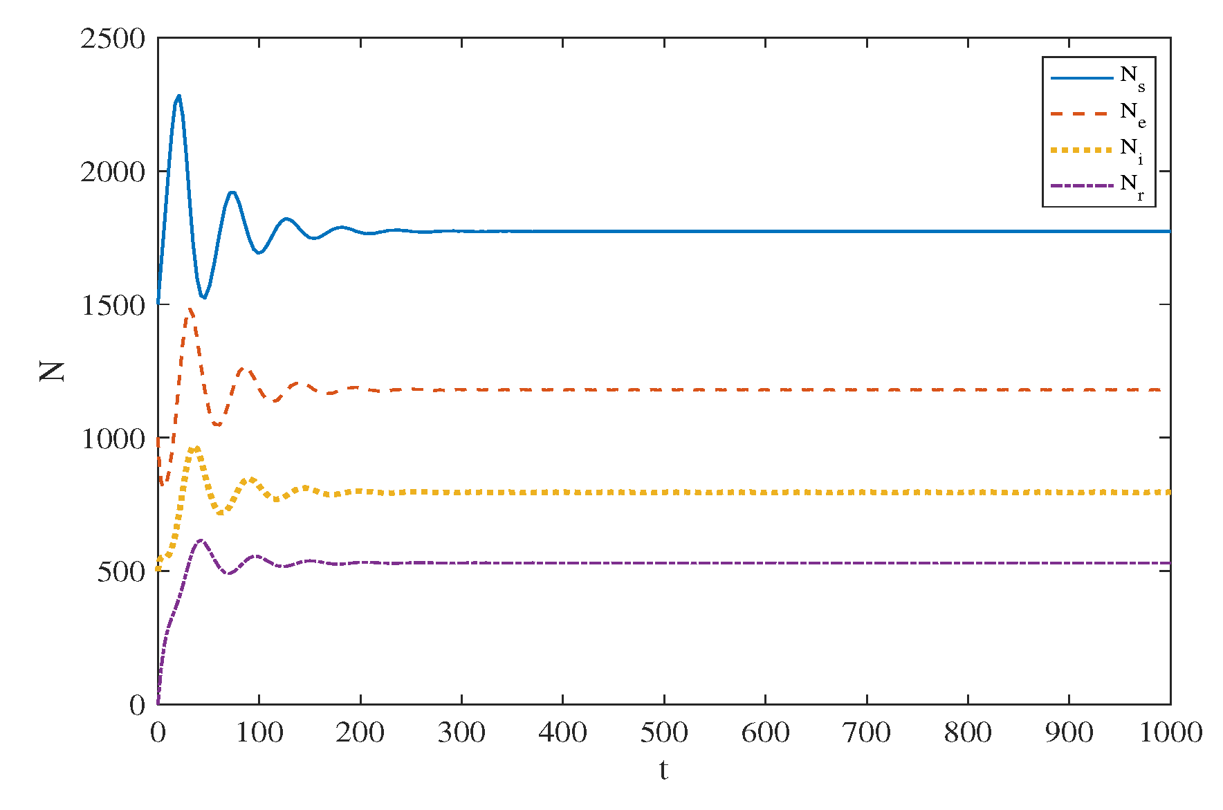
Next, we considered the endemic equilibrium point H * = ( N s * , N e * , N i * , N r * ) with τ = 0 . Let α i 0 = 0.13 , i = 1 , 2 , 3 , 4 ; μ 1 = 0.6 ; μ 2 = 0.5 ; μ 3 = 0.5 ; μ 4 = 0.3 ; θ 10 = 0.4 ; θ 20 = 0.1 ; θ 30 = 0.1 ; θ 40 = 0.2 ; γ 10 = 0.1 ; γ 20 = 0.15 ; γ 30 = 0.1 ; β 0 = 0.0023 ; p 0 = 0.1 ; q 0 = 0.15 ; ρ 0 = 0.02 ; and the initial value was ( N s ( 0 ) , N e ( 0 ) , N i ( 0 ) , N r ( 0 ) ) = ( 1500 , 1000 , 500 , 0 ) . The parameters of the system in Equation (20) satisfy the condition in Equation (36). The result is presented in Figure 2, which comes from Theorem 4; the system in Equation (20) has a unique endemic equilibrium point H * = ( N s * , N e * , N i * , N r * ) ( 1723 , 1108 , 797 , 531 ) and the system in Equation (20) is locally asymptotically stable.
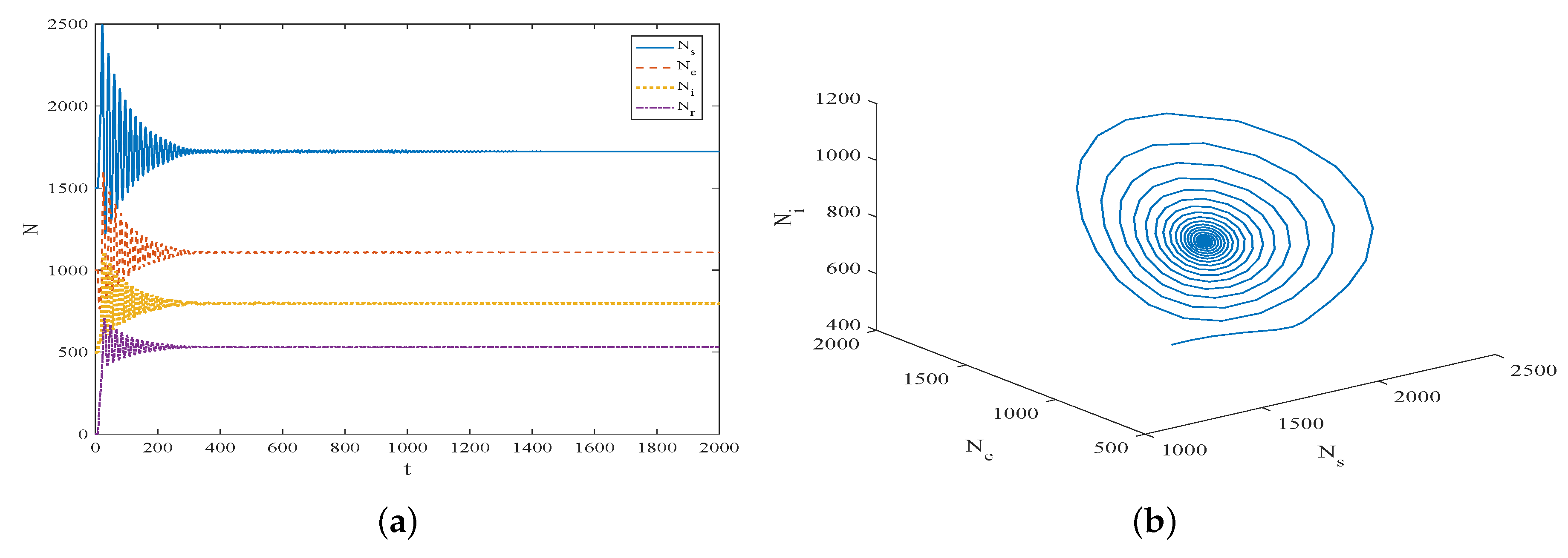
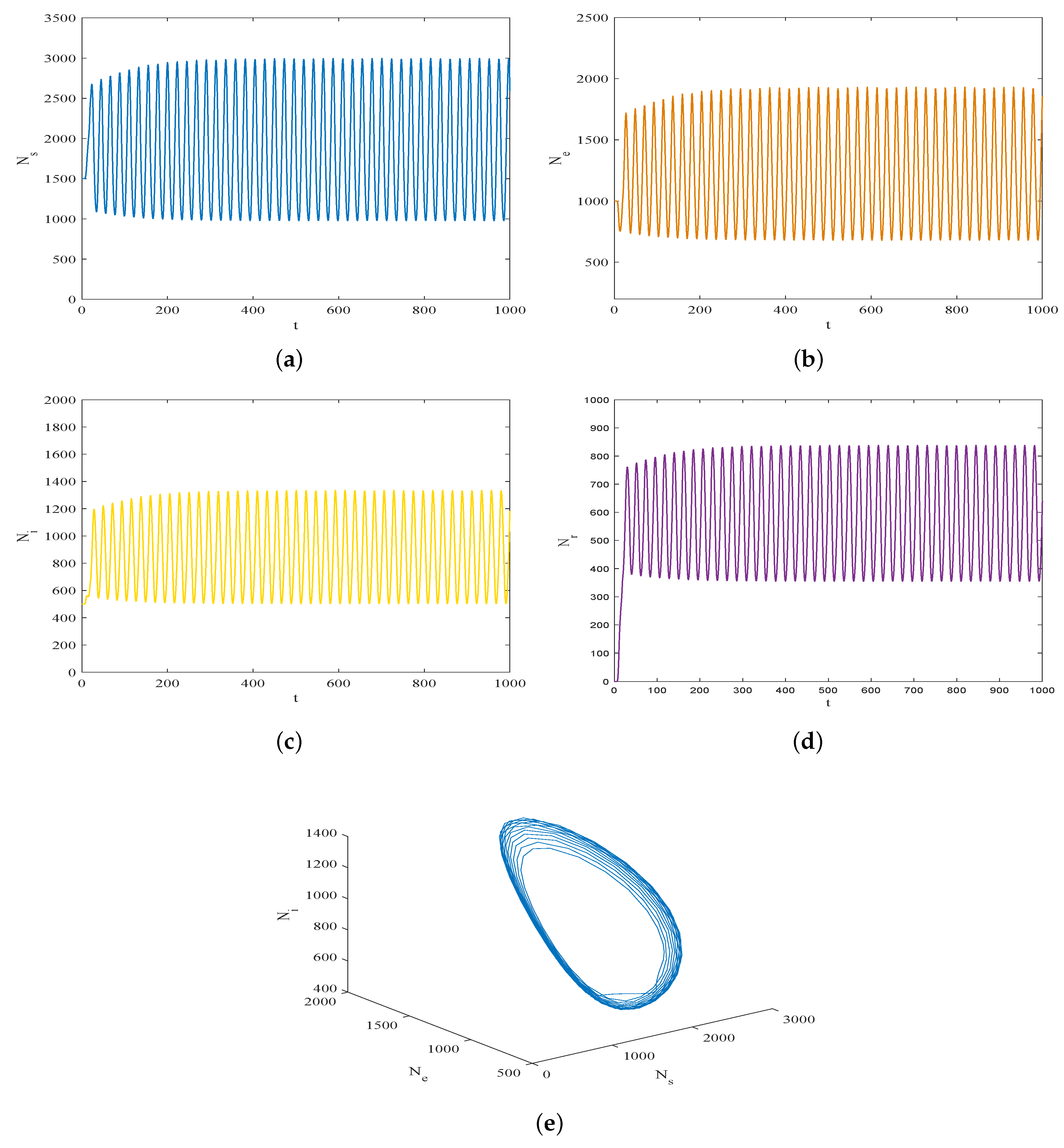
Similarly, let α i 0 = 0.13 , i = 1 , 2 , 3 , 4 ; μ 1 = 0.6 ; μ 2 = 0.5 ; μ 3 = 0.5 ; μ 4 = 0.3 ; θ 10 = 0.4 ; θ 20 = 0.1 ; θ 30 = 0.1 ; θ 40 = 0.2 ; γ 10 = 0.1 ; γ 20 = 0.16 ; γ 30 = 0.1 ; β 0 = 0.0023 ; p 0 = 0.1 ; q 0 = 0.15 ; ρ 0 = 0.02 ; and the initial value be ( N s ( 0 ) , N e ( 0 ) , N i ( 0 ) , N r ( 0 ) ) = ( 1500 , 1000 , 500 , 0 ) . In other words, N s ( 0 ) < N s * , N e ( 0 ) < N e * , N i ( 0 ) < N i * , and N r ( 0 ) < N r * . The parameters of the system in Equation (20) satisfy the conditions in Equations (43) and (44). In this case, we have the roots of Equation (41) are x 1 = 0.1398 , x 2 =0.0073, and x 3 , 4 = 0.213 ± 0.0248 i . Thus, we get x 0 = 0.0073 , ω 0 = 0.0855 , τ 0 = 5.3526 , and τ 1 = 73.4875 . The population dynamic behaviors of the endemic equilibrium point H * are shown in Figure 3 ( τ = 4.3526 ) and Figure 4 ( τ = 6.3526 ), respectively. It can been shown that the endemic equilibrium point H * spends longer time to become locally asymptotically stable only when 0 < τ < τ 0 (see Figure 3). When τ > τ 0 , it is quite clear that larger values of the time delay causes periodic oscillations. The equilibrium point loses its stability. Thus, the solution of the system in Equation (20) is unstable with the increase of time t (see Figure 4).

6. Concluding Remarks

In this article, the theory of an age-structured SEIRS model with time delay is analyzed. The model is based on the delayed nonlinear partial differential equation of initial-boundary value problems. The traveling wave solution of the system in Equation (1) is obtained using the method of characteristic and the recurrent algorithm. Then, we can obtain the existence and uniqueness of the continuous traveling wave solution of system according to hypotheses. The age-structured SEIRS model with time delay is reduced to a nonlinear ordinary differential equation under some insufficient simplifications. This allows us to obtain some sufficient conditions of existence of two equilibrium points of an age-structured SEIRS system: R 1 is a dimensionless index for the existence of the disease-free equilibrium point H 0 . R 2 , R 3 , and R 4 are dimensionless indexes for the existence of the endemic equilibrium point H * . From the biological point of view, the endemic equilibrium point H * only exists in the case of high values of death and conversion rate of exposed and infected population. The disease-free equilibrium point H 0 and the endemic equilibrium point H * are given. The disease-free equilibrium point H 0 = ( 0 , 0 , 0 , 0 ) is locally asymptotically stable if R 1 < 1 , R 2 < 1 , and R 3 < 1 . The stability of the endemic equilibrium point H * = ( N s * , N e * , N i * , N r * ) with τ = 0 and τ > 0 are analyzed: for R 0 > 1 , if the condition in Equation (36) holds, the endemic equilibrium point H * is locally asymptotically stable when τ = 0 ; if the conditions in Equations (43) and (44) hold, the endemic equilibrium point H * is locally asymptotically stable when time delay 0 < τ < τ 0 ; if the conditions in Equations (43)–(44) hold, the endemic equilibrium point H * is unstable when τ satisfies τ > τ 0 ; Hopf bifurcation occurs at τ = τ k ( k = 0 , 1 , 2 , ) . When time delay exceeds the critical value τ 0 , the system in Equation (20) loses its stability and Hopf bifurcation occurs. In this case, the susceptible, exposed, infected, and recovered population in the model will coexist in an oscillating mode and infectious diseases will get out of control. It can be seen that time delay has an important effect on the spread of infectious diseases. Therefore, we should shorten the time delay as much as possible in order to predict and eliminate infectious diseases. Our further research is using some bifurcation control strategies to control the occurrence of the Hopf bifurcation so as to control the occurrence of infectious diseases.
In general, this study provides the practical understanding of the different dynamic behaviors of an age-structured susceptible–exposed–infected–recovered–susceptible model with time delay, which is helpful for us to understand the application of epidemiology better in real life.

Supplementary Materials

The following are available online at https://www.mdpi.com/2227-7390/8/3/455/s1, Program S1: Software source code for Figure 1, Figure 2, Figure 3 and Figure 4.

Author Contributions

Conceptualization, Z.Y.; Funding acquisition, Y.Y.; Methodology, Z.Y.; Software, Z.Y. and Z.L.; and Supervision, Y.Y. All authors have read and agreed to the published version of the manuscript.

Funding

This work was supported by the National Nature Science Foundation of China (No. 61772063) and Beijing Natural Science Foundation (No. Z180005).

Acknowledgments

The authors would like to thank for the support funds.

Conflicts of Interest

The authors declare that there are no conflicts of interest regarding the publication of this paper.

References

  1. Kermack, W.O.; McKendrick, A.G. A contribution to the mathematical theory of epidemics. Proc. R. Soc. Lond. A 1927, 115, 700–721. [Google Scholar] [CrossRef] [Green Version]
  2. Brauer, F.; Castillo-Chavez, C. Mathematical Models in Population Biology and Epidemiology; Springer: New York, NY, USA, 2012. [Google Scholar]
  3. Zhou, X.; Cui, J.A. Analysis stability and bifurcation for an SEIR epidemic model with saturated recovery rate. Commun. Nonliear Sci. Numer. Simul. 2011, 16, 4438–4450. [Google Scholar] [CrossRef]
  4. Chauhan, S.; Misra, O.P.; Dhar, J. Stability Analysis of SIR Model with Vaccination. J. Comput. Appl. Math. 2014, 4, 17–23. [Google Scholar]
  5. Vargas-De-Len, C. On the global stability of SIS, SIR and SIRS epidemic model with standard incidence. Chaos Solitons Fractals 2011, 44, 1106–1110. [Google Scholar] [CrossRef]
  6. Shaikhet, L. Stability of SIR Epidemic Model Equilibrium Points; Springer: Berlin/Heidelberg, Germany, 2013. [Google Scholar]
  7. Chen, L.J.; Sun, J.T. Global stability and optimal control of an SIRS epidemic model on heterogeneous networks. Physica A 2014, 15, 196–204. [Google Scholar] [CrossRef]
  8. Lakshmanan, M.; Senthilkumar, D.V. Dynamics of Nonlinear Time-Delay Systems; Springer: Berlin/Heidelberg, Germany, 2010; p. 313. [Google Scholar]
  9. Smith, H. An Introduction to Delay Differential Equations with Application to the Life Sciences; Springer: Berlin/Heidelberg, Germany, 2011; p. 172. [Google Scholar]
  10. Sharma, S.; Mondal, A.; Pal, A.K.; Samanta, G.P. Stability analysis and optimal control of avian influenza virus A with time delays. Int. J. Dyn. Control 2018, 6, 1351–1366. [Google Scholar] [CrossRef]
  11. Xu, R.; Ma, Z.E.; Wang, Z.P. Global stability of a delayed SIRS epidemic model with saturation incidence and temporary immunity. J. Comput. Appl. Math. 2010, 59, 3211–3221. [Google Scholar] [CrossRef] [Green Version]
  12. Shu, H.Y.; Fan, D.J.; Wei, J.J. Global stability of multi-group SEIR epidemic models with distributed delays and nonlinear transmission. Nonlinear Anal. RWA 2012, 13, 1581–1592. [Google Scholar] [CrossRef]
  13. De la Sena, M.; Alonso-Quesadaa, S.; Ibeasb, A. On the stability of an SEIR epidemic model with distributed time-delay and a general class of feedback vaccination rules. Appl. Math. Comput. 2015, 270, 953–976. [Google Scholar] [CrossRef]
  14. Cooke, K.L.; Driessche, P. Analysis of an SEIRS epidemic model with two delays. J. Math. Biol. 1996, 35, 240–260. [Google Scholar] [CrossRef]
  15. Gao, S.J.; Chen, L.S.; Teng, Z.d. Impulsive Vaccination of an SEIRS Model with Time Delay and Varying Total Population Size. Bull. Math. Biol. 2007, 69, 731–745. [Google Scholar] [CrossRef] [PubMed]
  16. Wang, W.D. Global behavior of an SEIRS epidemic model with time delays. Appl. Math. Lett. 2002, 15, 423–428. [Google Scholar] [CrossRef]
  17. Schenzle, D. An age-structured model of pre-and post-vaccination measles transmission. IMA J. Appl. Math. 1984, 1, 169–191. [Google Scholar] [CrossRef] [PubMed]
  18. Metz, J.A.J.; Diekmann, O. The Dynamics of Physiologically Structured Populations. In Lecture Notes in Biomathematics; Springer: Berlin, Germany, 1986; p. 68. [Google Scholar]
  19. Iannelli, M. Mathematical Theory of Age-Structured Population Dynamics; Giardini Editorie Stampatori: Pisa, Italy, 1995. [Google Scholar]
  20. Hethcote, H.W. The mathematics of infectious diseases. SIAM Rev. 2000, 42, 599–653. [Google Scholar] [CrossRef] [Green Version]
  21. Mccluskey, C. Global stability for an SEI epidemiological model with continuous age-structure in the exposed and infectious classes. Math. Biosci. Eng. 2012, 9, 819–841. [Google Scholar]
  22. Zou, L.; Ruan, S.; Zhang, W. An age-structured model for the transmission dynamics of hepatitis B. SIAM J. Math. Appl. 2010, 70, 3121–3139. [Google Scholar] [CrossRef] [Green Version]
  23. Gandolfi, A.; Iannelli, M.; Marinoschi, G. An age-structured model of epidermis growth. J. Math. Biol. 2011, 62, 111–141. [Google Scholar] [CrossRef]
  24. Alexanderian, A.; Gobbert, M.K.; Fister, K.R.; Gaff, H.; Lenhart, S.; Schaefer, E. An age-structured model for the spread of epidemic cholera. Nonlinear Anal. RWA 2011, 12, 3483–3498. [Google Scholar] [CrossRef] [Green Version]
  25. Akimenko, V.V. Asymptotically stable states of non-linear age-structured monocyclic cell population model I. Travelling wave solution. Math. Comput. Simul. 2017, 133, 2–23. [Google Scholar] [CrossRef]
  26. Akimenko, V.V. Asymptotically stable states of non-linear age-structured monocyclic cell population model II. Numerical simulation. Math. Comput. Simul. 2017, 133, 24–38. [Google Scholar] [CrossRef]
  27. Akimenko, V.V. Nonlinear age-structured models of polycyclic population dynamics with death rates as a power functions with exponent n. Math. Comput. Simul. 2017, 133, 175–205. [Google Scholar] [CrossRef]
  28. Akimenko, V.V. An age-structured SIR epidemic model with fixed incubation period of infection. Math. Comput. Appl. 2017, 73, 1485–1504. [Google Scholar] [CrossRef]
  29. Guo, Z.K.; Huo, H.F.; Xiang, H. Global dynamics of an age-structured malaria model with prevention. Math. Biosci. Eng. 2019, 16, 1625–1653. [Google Scholar] [CrossRef] [PubMed]
  30. Huo, H.F.; Yang, P.; Xiang, H. Dynamics for an SIRS epidemic model with infection age and relapse on a scale-free network. J. Frankl. Inst. 2019, 356, 7411–7443. [Google Scholar]
  31. Diekmann, O.; Heesterbeek, J.A.P.; Metz, J.A.J. On the definition and the computation of the basic reproduction ratio R0 in models for infectious diseases in heterogeneous populations. J. Math. Biol. 1990, 28, 365. [Google Scholar] [CrossRef] [PubMed] [Green Version]
  32. Hassard, B.; Kazarinoff, N.; Wan, Y.H. Theory and Applications of Hopf Bifurcation; Cambridge University Press: London, UK, 1981. [Google Scholar]
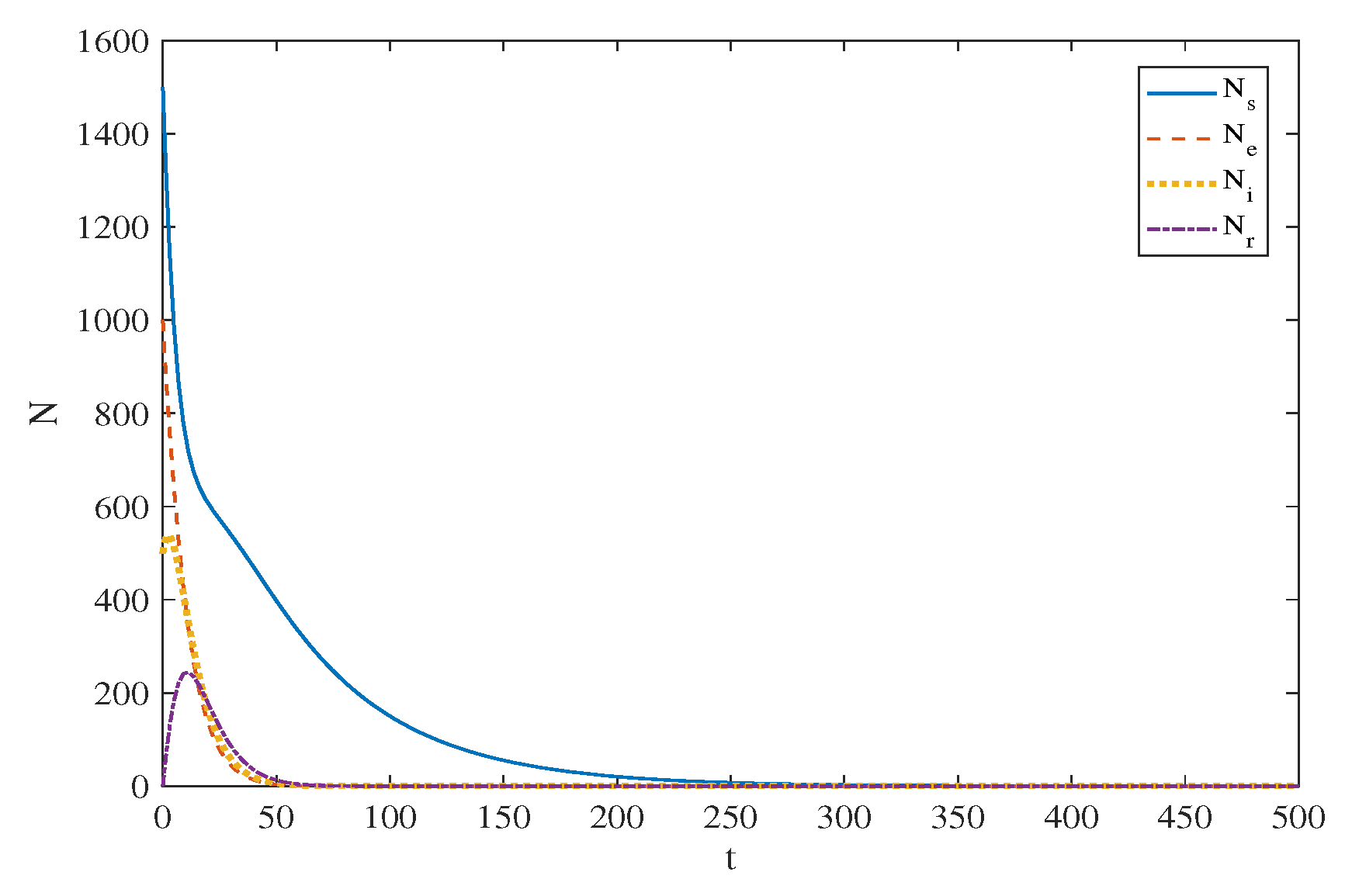
Figure 1. Local asymptotic stability of the disease-free equilibrium point H 0 = ( 0 , 0 , 0 , 0 ) .
Mathematics 08 00455 g001
Figure 2. Local asymptotic stability of the endemic equilibrium point H * = ( N s * , N e * , N i * , N r * ) when τ = 0 .
Mathematics 08 00455 g002
Figure 3. Local asymptotic stability of the endemic equilibrium point H * = ( N s * , N e * , N i * , N r * ) when τ = 4.3526 < τ 0 . (a) Time response diagram of N s , N e , N i and N r ; (b) Phase diagram of N s , N e and N i .
Mathematics 08 00455 g003
Figure 4. Instability of the endemic equilibrium point H * = ( N s * , N e * , N i * , N r * ) when τ = 6.3526 > τ 0 . (a) Time response diagram of N s ; (b) Time response diagram of N e ; (c) Time response diagram of N i ; (d) Time response diagram of N r ; (e) Phase diagram of N s , N e and N i .
Mathematics 08 00455 g004