An Optimization Model for the Temporary Locations of Mobile Charging Stations

Abstract

A possible solution with which to alleviate the range anxiety of electric vehicle (EV) drivers could be a mobile charging station which moves in different places to charge EVs, having a charging time of even half an hour. A problem that arises is the impossibility of charging in any location due to heavy traffic or limited space constraints. This paper proposes a new operational mode for the mobile charging station through temporarily stationing it at different places for certain amounts of time. A mathematical model, in the form of an optimization problem, is built by modeling the mobile charging station as a queuing process, the goal of the problem being to place a minimum number of temporary service centers (which may have one or more mobile charging stations) to minimize operating costs and the charger capacity of the mobile charging station so that the service offered is efficient. The temporary locations obtained are in areas with no or few fixed charging stations, making the mobile station infrastructure complementary to the fixed charging station infrastructure. The temporary location operational mode, compared to current moving operational mode, is more efficient, having a small miss ratio, short mean response time and short mean queuing time.

1. Introduction

The market for electric vehicle charging stations has grown rapidly in recent years. At present, the most developed markets for electric vehicle (EV) charging stations are in North America and Europe, with prospects for the Asian-Pacific market, in the near future (

Table 1. Sales of charging stations (thousands), 2012–2017.

Region	2012	2013	2014	2015	2016	2017
Africa/Middle East	<15	<20	<25	<40	<50	∼50
Asia Pacific	∼200	∼350	∼650	∼800	∼950	∼1000
Europe	∼75	∼200	∼240	∼350	∼450	∼500
Latin America	<5	<5	<10	<15	<25	<25
North America	∼70	∼200	∼260	∼350	∼400	∼450

Source: Global EV Outlook 2017 [1].

). Markets for EV charging stations are dependent on the state of their adoption, and the objectives and legislative targets in the region, which means that the market for charging stations for electric vehicles is higher in regions where electric cars are widely adopted. Some major problems faced by charging station infrastructure include its location and size, these two issues being extensively studied in the literature.

In the European Union, in 2019, it is estimated that approximately 165,064 charging stations were installed [2]. At present, there are no leaders in the charging station market, but the competitive market in the field is emerging through new, specialized companies, so there are opportunities for larger societies to own big market shares. In Europe, the electrical capacity of an electric car battery is approximately 20 kWh, which allows you to have a range of approximately 150 km [3]. Hybrid vehicles have a capacity of about 3–5 kWh for a range between 20 and 40 km. As this range is still limited, the vehicle battery should be recharged periodically. For a normal load (3 kW), vehicle manufacturers have developed a charger inside the car. For fast charging (22 kW, even 43 kW or more), manufacturers have developed two solutions: the use of a car charger designed to charge between 3 and 43 kW at single-phase (230V) or three-phase (400V) voltage (using an external charger that converts the alternating current to DC and charges the vehicle to 50 kW) [4].

Table 2. Charging time of an EV according to charger type.

Charging Time	Type of Source (kW)	Tension (V)	Maximum Current (A)	Mode
6–9 h	mono-phase 3.3 kW	230 V AC	16 A	Mode 1
2–3 h	triple-phase 10 kW	400 V AC	16 A	Mode 1
3–4 h	mono-phase 7 kW	230 V AC	32 A	Mode 2
20–30 min	triple-phase 43 kW	400 V AC	63 A	Mode 3
20–30 min	voltage continues 50 kW	400–500 V DC	100–125 A	Mode 4
1–2 h	triple-phase 24 kW	400 V AC	32 A	Mode 2

Source: IEC 61851-1 standard [4].

shows the charging time for an EV, depending on the type of connection.

According to IEC 61851-1 standard, the electric vehicle conduction stations can be made in four ways (Table 2) as follows:

• Mode 1 (L1) is the simplest EV charging solution. In this case, an EV is connected to AC power supply using standard sockets, but it must contain a contractor to disconnect the power supply in case of overload or an electric shock. The EV’s charging is done without communication between it and the station, and the maximum current accepted is 16 A.
• Mode 2 (L2), where the EV is charged from the power supply using standardized single-phase or three-phase sockets and charging conductors containing a box of control integrated into the cable with a pilot function command and a protection system against electrical shocks (RCD). The charge current value should not exceed 32 A.
• Mode 3 (L3), where an EV is connected via a specific scheme to the charging station (EAVE) that has installed control and protection functions. The maximum current is 3 × 63 A.
• Mode 4 (L4), where EVs are charged from stations using direct current.

Another obstacle in the development of EV market is range anxiety. Depending on the style of driving, the outside temperature and the traffic, the distance an EV can travel decreases, requiring more frequent recharging.

In the initial phase of charging infrastructure’s development, a solution with which to alleviate range anxiety may be a mobile charging station which can move to different places to charge EVs, having a charging time of even less than half an hour (Table 2). Furthermore, the mobile charging station can also be used as a car attendant service.

Current, the operational mode of a mobile charging station involves moving it, on demand, within a certain service area to charge EVs, only staying in that location for the time of charging. Multiple operating strategies for this type of charging station can be considered; for example, the mobile station may move on the FIFO (first-in, first-out) or the NJN (nearest-job-next) principles [5]. Based on a recent study [5], the last strategy seems to be the most appropriate, a question of interest being, “What would be the optimal charger capacity of the mobile charging station?” A higher charger capacity implies a higher cost for a mobile charging station. Based on data and statistical methods, Huang et al. [5] proposed an optimum battery capacity of 40 kWh and a charge rate between 15 and 30 kW for an urban environment such as Singapore, in order to design a mobile charging station. The cost range per unit of a DC fast charging station is $10,000–$40,000, while its installation cost range per unit is $4000–$51,000 [6,7]. An estimated cost per unit of a mobile charging station is $40,000 [5].

A problem that arises is the impossibility to charge in any location due to heavy traffic or limited space constraints. For example, in 2019, Gong et al. [8] adopted the concept of reasonable location in a location problem for fixed charging stations. A reasonable location is defined as “a location having a insignificant variance in the access frequencies to different charging stations” [8].

This paper proposes a new operational mode of the mobile charging station by temporarily stationing it, on demand, in different locations. A real frame, using data from New York taxis, is considered. A mathematical model, in the form of an optimization problem, is built by modeling the mobile charging station as a queuing process and the charging requests as Poisson processes. Furthermore, this optimization problem can also be used to position fixed charging stations. The purpose of the problem is to place a minimum number of temporary service centers (which may have one or more mobile charging stations) in order to minimize the operating costs and the charger capacity of the mobile charging station so that the service offered is effective, meaning, for example, that upon arrival at a service center, each EV will stand in a queue with no more than b clients with a probability of at least $\beta$.

Looking from the perspective of a company that operates the mobile charging stations, the company is interested in each service center having a queue of at least a clients with a probability of at least $\alpha$. The two queuing conditions mentioned can be combined so that in each service center we have at least a clients and at most b clients with a probability of at least $\gamma$.

The mobile charging station is not intended to be the main charging method for electric vehicles but a supplement to the fixed charging station, especially in areas where there are few or no fixed charging stations. Moreover, in countries with old electricity grid infrastructure (for example, Romania) a mobile charging station could take over the increased electricity demand due to the penetration of electric vehicles in the market until the modernization of the electricity distribution network infrastructure and until the installation of sufficient fixed stations. The mobile charging station is complementary to the fixed station in the incipient phase of developing charging station infrastructure.

The paper is structured in the following way. Section 2 is dedicated to a literature review. In Section 3, the proposed new operational mode of the mobile charging station is presented. Additionally, in this section, a mathematical model is discussed. Section 4 deals with estimating the optimization problem parameters. Section 5 discusses the results obtained from simulations using the New York taxi database [9], and in Section 6 we compare two operational modes of a mobile charging station. The paper is concluded in Section 7.

2. Literature Review

The power management of a mobile charging station was investigated in [10], considering Internet-of-Things to manage its supply power. The routing problem that arises with the current operational mode of a mobile charging station was also analyzed in the literature. Two decisions (location and routing) with time-windows were investigated in [11], with the results showing a need for a more efficient service in the sense of improving the charging rate or increasing battery capacity. Similar results were obtained by Cui et al. in 2018 [12] by modeling the routing problem of a mobile charging station as a mixed-integer linear problem with time windows. In [13], heterogeneous networks were used to optimally schedule the EV’s charge requests, assuming that EV users send their respective power demands and locations, when requesting battery recharging, to the mobile charging station.

In 2012, Jia et al. [14] considered several factors in the location of fixed charging stations, including demand for charging stations, driver behavior, road structure, fixed construction costs and operating costs, building a mathematical model that minimizes the total cost of investment. Additionally, charging infrastructure planning was discussed in [15] using multiday travel data. Zhu et al. [16] considered charging station location for plug-in EVs by minimizing the total cost of investment and how many chargers a charging station should have. Recently, in 2019, a two-level charging station locating method, which uses weighted multicriteria methods, was considered for locating charging stations [17].

Some studies take into consideration queuing time for the location problems of charging stations (for example, in [18,19,20,21,22]); various studies revealed that queuing time strongly affects the adoption of EVs [23,24]. Fast-charging stations have been proposed to address this issue; however, the installation of this type of charging station has a negative impact on the distribution network, such as high voltage [19,25] and overload distribution system during peak hours [26,27]. User behavior was considered in [28], while in [29] a resource planning scheme was investigated. An equilibrium modeling framework was considered in [30].

Other approaches consider the maximal covering location problem, taking into account the existing charging infrastructure [31] for urban taxi drivers. Frade et al. (2011) [32] also considered a maximal covering model with daytime versus nightime charging demands. Long travel data is considered in [33,34]. A quality of service index is introduced in [35] in a location optimization problem with charging reliability constraints.

3. Mathematical Model

In this section, we describe the operational mode of a mobile charging station which considers the temporary locations of this type of charging station.

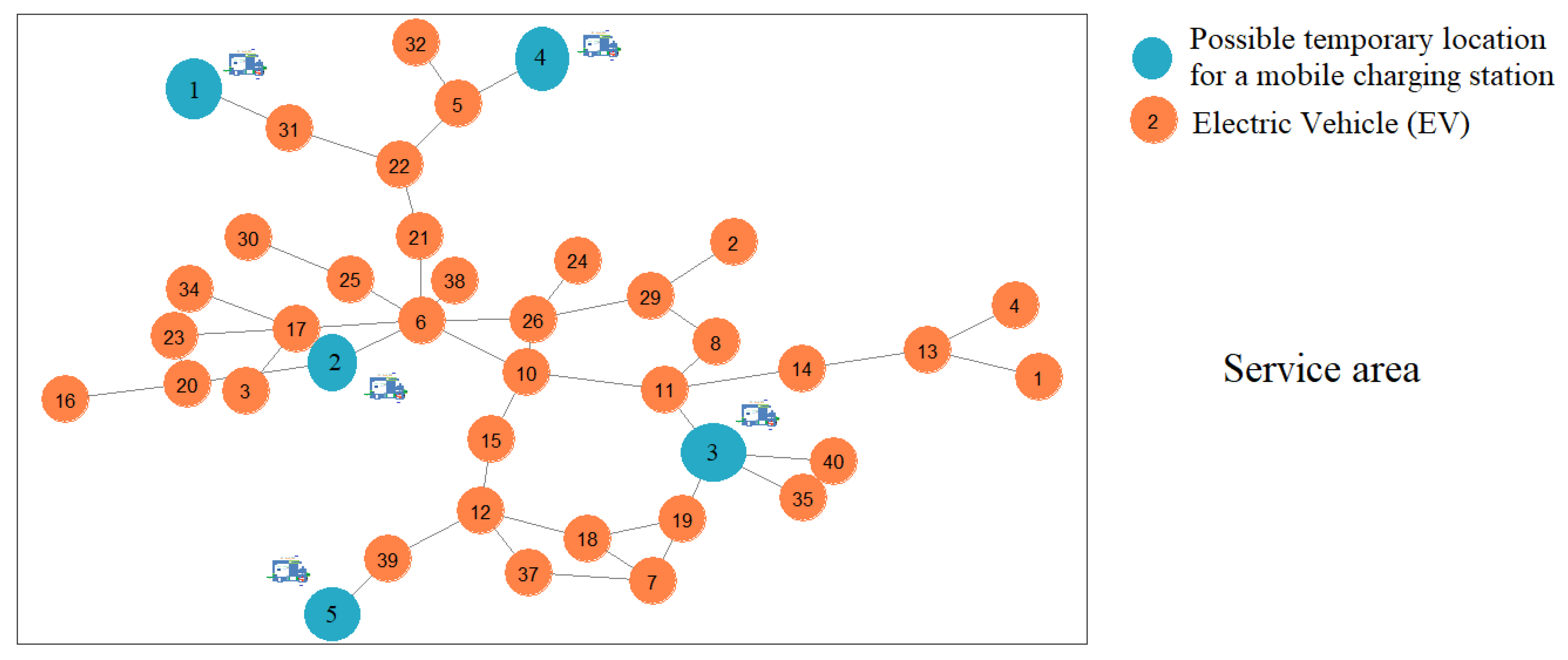
Suppose we have some places (depots) where the mobile charging station can stay. In these places, the mobile station charges both its own battery and the EVs’ batteries. Instead of moving the mobile station to where the electric vehicles that require the load are located, the mobile charging station stays for a period of time in a place, moving only between the location set, depending on the intensity of the demand in the depot areas within a certain time interval. Thus, a mobile charging station fulfills the functions of a stationary charging station and those of a mobile charging station. Examples of stationary stations of a mobile station can be gas stations and tramway heads. We no longer assume that the mobile station can move and load anywhere, but only in certain places (Figure 1). If there are many requests for a sub-zone, a mobile station stays there for a while, while another moves between places. Depending on the day and time (during the week or weekend), the mobile station stays for a while in a place, after which time it moves to another place. Through a smartphone application, EVs can see where the mobile station is stationed.

A charging station’s infrastructural development deals with constructing optimization problems considering budget constraints and capacity optimization [36,37]. Techniques used involve particle swarm optimization [38,39], the hybrid optimization algorithm [40], ant colony optimization [41] and the genetic algorithm [42,43].

This paper proposes a mixed linear optimization location-allocation problem of mobile charging stations based on a simulation.

In 1998 and 2002, Marianov and Serra [44,45] proposed a location-allocation problem considering queuing constraints in the form of queue length and waiting time of a customer. Similar constraints are considered in this paper.

The purpose of the optimization problem is to place a minimum number of temporary service centers for EVs’ charging, each center having a minimum number of mobile charging stations that can charge the EVs while minimizing the charger capacity of mobile charging stations required for running the service system in some optimal parameters (stated a priori) such that

(i)

Each EV will be assigned to a center at the shortest possible distance from its location.

(ii)

Upon arrival at the service center, each EV will stand in a queue with no more than b clients with a probability of at least $\beta$; or in each center will be at least a clients, with a probability of at least $\alpha$; or when arriving at the service center, each EV will be in a queue with no more than b clients, and in each center will be at least a clients, with a probability of at least $\gamma$.

(iii)

The battery capacity of the mobile charging station is enough to meet all requests during the considered temporary location period.

When a mobile charging station becomes idle, having no customers, it can be used in another service area. If a mobile charging station is not used in a service area, for a day or for several hours, it may be temporarily allocated to a service area lacking a mobile charging station; thus, the location and battery state of charge can take different values depending on the day, time and area.

The operating cost associated with a mobile charging station may be composed of the cost of the electricity required to charge the battery of the mobile charging station and maintenance costs.

3.1. Nonlinear Optimization Problem

The problem (P1), given below, minimizes the number of service centers; the number of mobile stations in each service center; the distances between the demand nodes and the locations of the mobile charging stations; and the charger capacity of the mobile charging station battery.

Optimization problem (P1):

$$\begin{array}{cc}\hfill min& \sum _{j\in J_1}\sum _{m=2}^{C_j}{z}_{jm}{P}_{jm}+\sum _{j\in J_1}{z}_{j1}{P}_{j1}+\sum _{i\in I}\sum _{j\in J}{d}_{ij}{x}_{ij}+\sum _{j\in J}\sum _{m=1}^{C_j}So{C}_{jm}{z}_{jm},\mathrm{where}J=J_1\cup J_2\hfill \end{array}$$

(1)

subject to the following constraints:

$$\sum _{j\in J}{x}_{ij}=1,\forall i\in I$$

(2)

$$z_{jm}\le z_{j1},j\in J_1,m=2,3,\dots ,C_j$$

(3)

$$x_{ij}\le z_{j1},\forall i\in I,j\in J$$

(4)

$$\sum _{j\in J_1}\sum _{m=1}^{C_j}{z}_{jm}=B$$

(5)

$$\sum _{m=1}^{C_j}So{C}_{jm}{z}_{jm}\ge \sum _{i\in I}{g}_i{x}_{ij},\forall j\in J$$

(6)

$$C_j=1,\forall j\in J_2$$

(7)

$$d_{ij}{x}_{ij}\le D,\forall i\in I,j\in J_2$$

(8)

$$\mathrm{P}[\mathrm{center}j\mathrm{has}\mathrm{at}\mathrm{most}b\mathrm{EVs}\mathrm{in}\mathrm{queue}]\ge \beta ,\forall j\in J$$

(9)

or

$$\mathrm{P}[\mathrm{center}j\mathrm{has}\mathrm{at}\mathrm{least}a\mathrm{EVs}\mathrm{in}\mathrm{queue}]\ge \alpha ,\forall j\in J$$

(10)

or

$$\mathrm{P}[\mathrm{center}j\mathrm{has}\mathrm{at}\mathrm{least}a\mathrm{EVs}\mathrm{and}\mathrm{at}\mathrm{most}b\mathrm{EVs}\mathrm{in}\mathrm{queue}]\ge \gamma ,\forall j\in J$$

(11)

$$x_{ij},z_{jm}\in \{0,1\},\forall j\in J,m=1,2,\cdots ,C_j$$

(12)

$$So{C}_{jm}\mathrm{positive}\mathrm{integer},So{C}_{jm}\le {\omega }_u,\forall j\in J,m=1,2,\cdots ,C_j$$

(13)

$$B\mathrm{positive}\mathrm{integer},B\le B_{max}$$

(14)

Constraint (2) is allocated to every node a single service center, while constraint (3) limits the number of mobile stations to $C_j$ and indicates that mobile charging station m cannot be placed at node j without first placing ${(m-1)}^{th}$ mobile station. We force the allocation of a demand node to an open service center by constraint (4); $z_{j1}$, for $j\in J_2$ takes the value 1 when node i is assigned to fixed charging station from node $j\in J_2$. The maximum number of mobile charging station which can be placed is B (constraint (5)). The total charging capacity of service center j having at most $C_j$ mobile charging stations is greater than or equal to the sum of the average charge load required from node i satisfied by the center j (constraint (6)). Constraint (7) refers to fixed charging stations, assuming the existence of just one fixed charging station in node $j\in J_2$. Additionally, we assume that nodes i cannot be assigned to a fixed charging station located more than D km away (Equation (8)). The decision variables of problem (P1) are $z_{jm}$, $x_{ij}$, B and $So{C}_{jm}$.

Upon arrival at the serving center, each EV will stand in queue with no more than b clients with a probability of at least $\beta \in (0,1)$ (Equation (9)); or in each center there will be at least a clients with a probability of at least $\alpha \in (0,1)$ (Equation (10)); or when arriving at the service center, each EV will stand in queue with no more than b clients, and in each center there will be at least a customers, with a probability of at least $\gamma \in (0,1)$ (Equation (11)).

Due to the fact that the optimization problem (P1) is nonlinear, we define the equivalent mixed linear problem to (P1) in the following way.

3.2. Linear Optimization Problem

The equivalent mixed linear problem (P2) is given by

$$\begin{array}{cc}\hfill min& \sum _{j\in J_1}\sum _{m=2}^{C_j}{z}_{jm}{P}_{jm}+\sum _{j\in J_1}{z}_{j1}{P}_{j1}+\sum _{i\in I}\sum _{j\in J}{d}_{ij}{x}_{ij}+\sum _{j\in J}\sum _{m=1}^{C_j}So{C}_{jm}\hfill \end{array}$$

(15)

subject to constraints (2), (3), (4), (5), (7), (8), (9) or (10) or (11), (12), (13), (14) and

$$\sum _{m=1}^{C_j}So{C}_{jm}\ge \sum _{i\in I}{g}_i{x}_{ij},\forall j$$

(16)

$$So{C}_{jm}\le z_{jm}{\omega }_U,\forall j\in J,m=1,2,3,\dots ,C_j$$

(17)

If $z_{jm}$ is 0, then $So{C}_{jm}$ is 0. If $z_{jm}$ is 1, then $So{C}_{jm}$ cannot be greater than the maximum charger capacity ${\omega }_U$. The decision variables of problem (P2) are $z_{jm}$, $x_{ij}$, B and $So{C}_{jm}$.

Constraint (9) can be rewritten according to the intensity of requests in nodes i and the mean serving rate of the mobile charging stations in nodes j. Assuming that the charge requests from each node i follow a Poisson process of intensity $f_i$ and that the serving time is exponentially distributed with an mean serving rate of ${\mu }_j$, condition (9) is equivalent to the following linear condition (for mobile charging stations) [44,46]

$$\sum _{i\in I}{f}_i{x}_{ij}\le {\mu }_j[z_{j1}{\rho }_{\beta j1}+\sum _{m=2}^{C_j}{z}_{jm}({\rho }_{\beta jm}-{\rho }_{\beta j(m-1)})],$$

(18)

$\forall j\in J_1$, where the values ${\rho }_{\beta jm}$ are determined a priori from the following inequality

$$\sum _{k=0}^{m-1}\frac{(m-k)m!m^b}{k!}\frac{1}{{\rho }^{m+b+1-k}}\ge \frac{1}{1-\beta },$$

(19)

those being the values for which in (19) we have equality, while for fixed charging stations we have the equivalent linear condition

$$\sum _{i\in I}{f}_i{x}_{ij}\le {\mu }_j{z}_{j1}{\rho }_{\beta j1},j\in J_2$$

(20)

Fixed values of ${\rho }_{\beta jm}$ are computed for every possible level of probability-chosen $\beta$, provided there are m mobile charging stations at node j.

Similarly, we obtain the following new result for constraint (10) which is equivalent to the following linear condition (for mobile charging station)

$$\sum _{i\in I}{f}_i{x}_{ij}\ge {\mu }_j[z_{j1}{\theta }_{\alpha j1}+\sum _{m=2}^{C_j}{z}_{jm}({\theta }_{\alpha jm}-{\theta }_{\alpha j(m-1)})],$$

(21)

$\forall j\in J_1$, where the values ${\theta }_{\alpha jm}$ are determined a priori from the following inequality:

$$\sum _{k=0}^{m-1}\frac{(m-k)m!m^a}{k!}\frac{1}{{\theta }^{m+a+1-k}}\le \frac{1}{\alpha }$$

(22)

The equivalent linear condition for fixed charging station infrastructure is

$$\sum _{i\in I}{f}_i{x}_{ij}\ge {\mu }_j{z}_{j1}{\theta }_{\alpha j1},j\in J_2$$

(23)

Fixed values of ${\theta }_{\alpha jm}$ are computed for every possible level of probability-chosen $\alpha$ provided there are m mobile charging stations at node j. The equivalence of inequality (22) to constraint (10) is given by the next theorem.

Theorem 1.

Constraint $\theta \ge {\theta }_{\alpha }$, where ${\theta }_{\alpha }$ is the value for which in Equation (22) holds equality, is equivalent to constraint (10).

Inequality (22) is equivalent to (10), i.e., Theorem 1 holds, and because $\theta$ can be rewritten as a function of variables $x_{ij}$, it yields linear deterministic constraints (21) with ${\theta }_{\alpha jm}$ such that (22) holds as an equality.

A linear form of condition (11) can be obtained similarly to those obtained for (9) and (10). Assuming service times in each service center are exponentially assigned with a mean serving rate ${\mu }_j>0$, to have a balance in the system, we have the condition ${\mu }_j\ge m_j{\lambda }_j$ where $m_j$ represents the number of mobile stations of center j, and ${\lambda }_j$ is the intensity of the Poisson process of charge requests arriving to center j. Marianov and Serra [45] showed that

$${\lambda }_j=\sum _{i\in I}{f}_i{x}_{ij}$$

Assuming that each service center is represented by a M/M/m queuing process, we can calculate the probability from (11). Assuming that the two events are independent, this probability can be written as

$$\begin{array}{c}\mathrm{P}\left[\mathrm{center}j\mathrm{has}\mathrm{at}\mathrm{least}a\mathrm{EVs}\mathrm{and}\mathrm{at}\mathrm{most}b\mathrm{EVs}\mathrm{in}\mathrm{queue}\right]=\mathrm{P}[\mathrm{center}j\mathrm{has}\mathrm{at}\mathrm{least}a\mathrm{EVs}\mathrm{in}\mathrm{queue}\times \\ \mathrm{P}[\mathrm{center}j\mathrm{has}\mathrm{at}\mathrm{most}b\mathrm{EVs}\mathrm{in}\mathrm{queue}\end{array}$$

The assumption of independence leads to an approximation of reality, but ease of calculus. In a future paper we will address the issue of dependence.

We want the probability of an EV arriving at a center to find a queue with less than b other EVs, and the probability that the queue length at a center is greater than a EVs.

The first probability can be written as $1-(p_{m+b+1}+p_{m+b+2}+\dots +p_{\infty })$, and the second is $p_{m+a+1}+p_{m+a+2}+\dots +p_{\infty }$, while $p_{m+1}$ are the state probabilities of the system, where a state $m+1$ corresponds to the event when we have $m+1$ EVs at the center, one EV being in the queue waiting to be recharged, while the others are recharged; for a state $k\le m$, we have k EVs being recharged at a service center. In the following, we will drop the indices for a easier reading.

Expressions for the state probabilities are the following [47]:

$$p_k=p_0{\omega }^k/k!,k\le m$$

$$p_k=p_0{\omega }^k/m!m^{k-m},k>m$$

$$p_0={(\frac{{\omega }^m}{(1-{\displaystyle \frac{\omega }{m}})m!}+\sum _{j=0}^{m-1}\frac{{\omega }^j}{j!})}^{-1}$$

where $\omega =\lambda /\mu$. With these formulae, Equation (11) becomes

$$\left[\frac{p_0{m}^m}{m!}{\left(\frac{\omega }{m}\right)}^{m+a+1}\frac{1}{1-{\displaystyle \frac{\omega }{m}}}\right]\times [1-\frac{p_0{m}^m}{m!}{\left(\frac{\omega }{m}\right)}^{m+b+1}\frac{1}{1-{\displaystyle \frac{\omega }{m}}}]\ge {\gamma }_j,\forall j\in J$$

(24)

Replacing $p_0$ and after some calculus, we get

$$\begin{array}{cc}\hfill & \sum _{j=0}^{m-1}\frac{(m-j)m!m^b}{j!}\frac{1}{{\omega }^{m+b+1-j}}-{\gamma }_j\sum _{j=0}^{m-1}\sum _{k=0}^{m-1}\frac{(m-j)(m-k){(m!)}^2{m}^{a+b}}{k!j!}\times \frac{1}{{\omega }^{2m+2+a+b-k-j}}\ge 1\hfill \end{array}$$

(25)

This equation is equivalent to Equation (11). However, due to it being a nonlinear equation, we require an equivalent linear equation.

We denote by ${\phi }_j:[0,1]\to \mathbb{R}$ the left hand side of Equation (25) which depends on $\omega$, for all $j\in J$. We prove that function ${\phi }_j\left(\omega \right)$ is increasing.

Lemma 1.

Function ${\phi }_j\left(\omega \right)$ is an increasing function for all $\omega \in [0,1]$ and for all

$${\gamma }_j\ge {\left[\sum _{k=0}^{m-1}\frac{(m-k)m!m^a}{k!}\frac{2m+2+a+b-k-j}{m+b+1-j}\right]}^{-1}$$

Proof. 

The derivative of ${\phi }_j\left(\omega \right)$ is

$${\phi }_j^{\prime }\left(\omega \right)=\sum _{j=0}^{m-1}\left\{\frac{(m-j)m!m^b(-1)}{j!}\frac{(m+b+1-j)}{{\omega }^{m+b+2-j}}\right[1-{\gamma }_j\sum _{k=0}^{m-1}\frac{(m-k)m!m^a}{k!}\frac{2m+2+a+b-k-j}{{\omega }^{m+a+1-k}(m+b+1-j)}\left]\right\}$$

We denote by $h_j:[0,1]\to \mathbb{R}$ function

$$\begin{array}{cc}\hfill h_j\left(\omega \right)& =1-{\gamma }_j\sum _{k=0}^{m-1}\frac{(m-k)m!m^a}{k!}\frac{2m+2+a+b-k-j}{{\omega }^{m+a+1-k}(m+b+1-j)}\hfill \end{array}$$

The derivative of function $h_j\left(\omega \right)$ is

$$\begin{array}{cc}\hfill & h_j^{\prime }\left(\omega \right)=-{\gamma }_j\sum _{k=0}^{m-1}\frac{(m-k)m!m^a}{k!}\frac{(-1)(m+a+1-k)(2m+2+a+b-j-k)}{{\omega }^{m+a+2-k}(m+b+1-j)}\hfill \end{array}$$

Because $m+a+1-k$ and $m+b+1-j$ are positive, like the rest of the terms, we obtain that $h_j^{\prime }\left(\omega \right)$ is positive. Hence, we get $h_j\left(\omega \right)$ is increasing. We have $\underset{\omega \to 0}{lim}{h}_j\left(\omega \right)=-\infty$, and

$$\begin{array}{cc}\hfill \underset{\omega \to 1}{lim}{h}_j\left(\omega \right)& =1-{\gamma }_j\sum _{k=0}^{m-1}\frac{(m-k)m!m^a}{k!}\frac{2m+2+a+b-j-k}{m+b+1-j}\hfill \end{array}$$

For

$${\displaystyle {\gamma }_j\ge {\left[\sum _{k=0}^{m-1}\frac{(m-k)m!m^a}{k!}\frac{2m+2+a+b-j-k}{m+b+1-j}\right]}^{-1},}$$

$j\le m-1$, we have that $\underset{\omega \to 1}{lim}{h}_j\left(\omega \right)\le 0$. Hence, $h_j\left(\omega \right)$ is negative, and as a consequence ${\phi }_j^{\prime }\left(\omega \right)$ is positive. Thus, we conclude that ${\phi }_j\left(\omega \right)$ is increasing for all $j\in J$. ☐

We choose $\gamma$ to be $\gamma =\underset{j\in J}{max}\left({\gamma }_j\right)$.

The equivalence of inequality (25) to constraint (11) is given by the next theorem.

Theorem 2.

Constraint $\omega \ge {\omega }_{\gamma }$, where ${\omega }_{\gamma }$ is the value for which in Equation (25) holds equality, is equivalent to constraint (11).

Proof. 

Let ${\omega }_{\gamma }$ be he value for which in Equation (25) we have equality. Because function ${\phi }_j\left(\omega \right)$ is increasing, then for any $\omega \ge {\omega }_{\gamma }$, Equation (25) is true. ☐

Therefore, once a value for $\gamma$ is chosen, we determine the value for ${\omega }_{\gamma }$ with any root-finding numerical method. The constraint (11) in optimization problem (P2) becomes (for mobile charging station):

$$\sum _{i\in I}{f}_i{x}_{ij}\ge {\mu }_j[z_{j1}{\omega }_{\gamma j1}+\sum _{m=2}^{C_j}{z}_{jm}({\omega }_{\gamma jm}-{\omega }_{\gamma j(m-1)})],$$

(26)

$\forall j\in J_1$, where values ${\omega }_{\gamma jm}$ are determined a priori from inequality (25), those being the values for which in this equation we have equalities. The equivalent linear constraint of (11) for fixed charging station is

$$\sum _{i\in I}{f}_i{x}_{ij}\ge {\mu }_j{z}_{j1}{\omega }_{\gamma j1},j\in J_2$$

(27)

Fixed values of ${\omega }_{\gamma jm}$ are computed for every possible level of probability-chosen $\gamma$, provided there are m mobile charging stations at node j.

Inequality (25) is equivalent to (11), i.e., Theorem 2 holds, and because $\omega$ can be rewritten as a function of variables $x_{ij}$, it yields linear deterministic constraints (26) with ${\omega }_{\gamma jm}$ such that (25) holds as equality.

4. Estimating Parameters

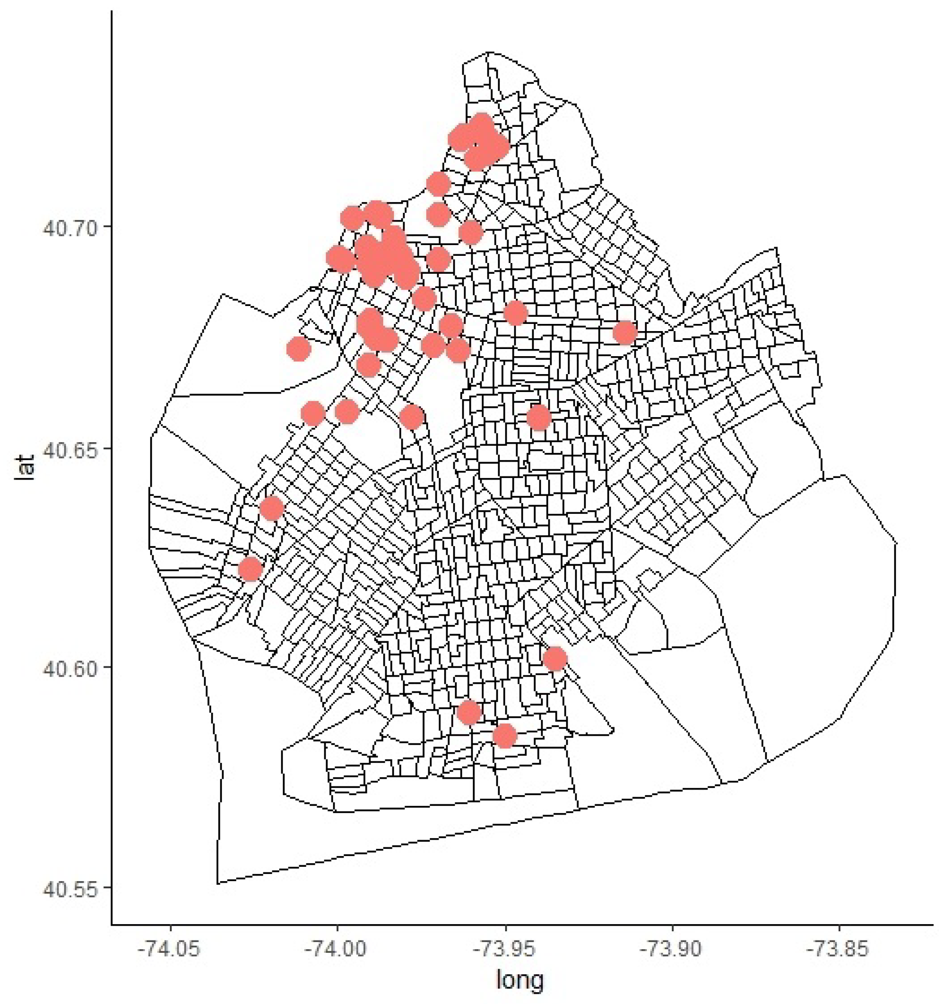
New York City, United States is one of the cities with the highest population densities, with a population of over 8 million in 2018 and an area of 784 km${}^2$. Therefore, the service area considered in this paper is restricted to one of its districts; namely, Brooklyn, New York (Figure 2 displays the fixed stations [48]). Most fixed charging stations are located in the north of Brooklyn, with very few being located to the south of it. Most of these are placed in parking lots, those being L2 level type charging stations (95%) (only three being the fast-charging type).

In this section, we estimate some parameters of the temporary placement problem of mobile charging stations based on data from [9]. The database, which we denote by NYC, refers to New York taxi trips in 2013. For each NYC record line we have the following attributes:

• Identity number of the taxi;
• Distance (miles) and trip time (seconds);
• Customer pick-up times and arrival times at destination (day, month, year, hour);
• Pick-up and destination locations of customers (latitude and longitude).

In order to develop the EV market, a solution, even temporary, is needed. This solution, in the case of Brooklyn and similar cases, may be the mobile charging station.

Estimating the parameters of the location problem involves, firstly, building a matrix of distances and trip driving speeds between the intersections of the service area. A first step is to associate each pickup and destination location with an intersection. Using the OpenStreetMap application, the distances from each location to each intersection are calculated. The pickup and destination locations are associated with the closest intersection. For each intersection i, the road distance and the duration of the trip to intersection j, are determined with OpenStreetMap. Based on these distances we determine the driving speed from intersection i to intersection j. In this way, we obtain the driving time from intersection i to intersection j, which we denote by $D_t^M(i,j)$.

Because energy consumption is influenced by traffic conditions, we determine how much time the taxi spends in traffic depending on the day of the week and the time of day. This is achieved with TomTom statistics [49]. These statistics tell us how much more time a car spends in traffic per day and hour, as a percentage. On Monday, there is heavy traffic between 15:00 and 16:00 and between 8:00 and 9:00, while on Saturday, there is heavy traffic in the evening between 17:00 and 20:00. Thus, we obtain the trip time from intersection i to intersection j which we denote by $D_t^T(i,j)$.

The idle trip time due to traffic conditions is given by

$$D_t^I(i,j)=D_t^T(i,j)-D_i^M(i,j)$$

(28)

Based on trip time, driving time and idle time, we can derive the energy consumed by the taxi for a trip from intersection i to intersection j. Similarly to [50,51], we estimate the energy consumption using a black-box approach using multiple linear regression. Hence, total energy consumption for a trip can be decomposed into moving energy consumption $E_i^M(i,j)$ and auxiliary loading energy consumption $E_t^A(i,j)$:

$$\begin{array}{cc}\hfill & E_t^T(i,j)=E_t^M(i,j)+E_t^A(i,j)\hfill \end{array}$$

(29)

$$\begin{array}{cc}\hfill & E_i^M(i,j)=\eta ({\alpha }_1{v}_t{(i,j)}^2+{\alpha }_2{v}_t(i,j)+{\alpha }_3)d_{ij}\hfill \end{array}$$

(30)

$$\begin{array}{cc}\hfill & E_t^A(i,j)=l_t{D}_t^T(i,j)/60\hfill \end{array}$$

(31)

where $v_t(i,j)$ represents the driving speed of a trip from intersection i to intersection j at time t (km/h) and $E_t^T(i,j)$ total energy consumption.

The value of the auxiliary parameter $l_t$ is dependent on the outside temperature, the battery storage capacity of an EV being affected by it. This value can be estimated based on historical weather data from New York City. Similarly to [50], we choose $l_t$ to be between 1 and 1.5.

The parameter $\eta$ is the aggressive factor of the car driver. As the driving is more aggressive, the EV consumes more energy. In contrast, a calm driver can save from 30% to 40% of the energy consumed in the event of aggressive driving [50]. We take $\eta =0.8$ (calm driving), $\eta =1$ (normal driving) and $\eta =1.2$ (aggressive driving) [50]. Based on [5,50], we have chosen the Nissan Leaf model to be the electric taxi car, for which we take ${\alpha }_1=0.1554$, ${\alpha }_2=-5.4634$ and ${\alpha }_3=189.297$.

In order to estimate some parameters of the optimization problem (P2) such as the Poisson intensity $f_i$, a simulation approach is applied. Therefore, a taxi simulation drive is performed which is based on destination probabilities for pickup intersection i, at time t. An hourly time interval is considered for deriving these probabilities. Using the NYC database, we determine the number of clients at intersection i for moment of time t (denoted by $N_t^P\left(i\right)$) and the number of clients who took a taxi from intersection i to intersection j (denoted by $N_t^D(i,j)$). The probability of picking up a client at intersection i, at time t, having as destination intersection j is given by:

$$P_{i/j}^D=\frac{N_t^D(i,j)}{N_t^P\left(i\right)}$$

(32)

These probabilities are transformed into a discrete distribution for each intersection and moment of time t. Destination intersection for a taxi located at intersection i and moment of time t are chosen according to a corresponding discrete distribution constructed assuming the following:

• The taxi has enough energy to make the trip.
• If for intersection i at time t there is no probability of a destination obtained from the NYC data, then all intersections have the same probability of destination.
• Discrete distributions are constructed so that intersections with high probabilities have greater chances of random choice than others. Intersections for which we did not have a destination probability in the data were considered to have the same probability.
• The taxi picks up a customer as soon as it reaches the next intersection.
• The maximum charge capacity of an electric taxi battery is 30 kW, taking the lower and upper limits as 5% and 95%.

Based on probabilities $P_{i/j}^D$, each trip $(i,j)$ is put into a category based on time intervals of an hour as follows: ≥0.5 strong chance of destination, $[0.2,0.5)$ medium high chance of destination, $(0,0.2)$ medium chance of destination and 0 low change of destination. The reason for not using just the probabilities $P_{i/j}^D$ is that at some point during the simulation, the program remained in only one intersection i that at a moment of time t had no probability of destination for any intersection j. For each intersection i we count the number of strong, medium-high, medium and low destination intersections. The probability of destination for a strong intersection is given by 0.5/number of strong intersections; for medium high it is 0.4/number of medium high intersections; for medium, 0.3/number of medium intersections; and for a low intersection is what is left to reach 1 over number of low intersections corresponding to pickup intersection i. In this manner, we construct discrete probability of destination for every pickup intersection i.

With these values, we can determine the intensity of charge requests $f_i$ in a certain area within a certain time-frame.

In the analysis, different types of mobile charging stations can be considered. Depending on this, the average serving time differs from a high charge rate to a longer service time.

5. Results and Discussions

Based on simulation performed and estimated parameters, we solved the optimization problem (P2) for different days and time-frames. A number of 200 taxis were simulated starting from different locations, 100 taxis of which started the working day at 6 o’clock, and the other 100 taxis started at 7 o’clock.

Considering that taxi drivers make the decision to recharge their electric taxis when they have less than 30% battery capacity, the intersections where these decisions were made were recorded. Because the number of intersections obtained may be quite large, a hierarchical clustering approach was used to cluster intersections by considering a maximum distance of 4 km from the cluster center [52,53]. We assume that the taxi driver’s style is normal ($\eta =1$). 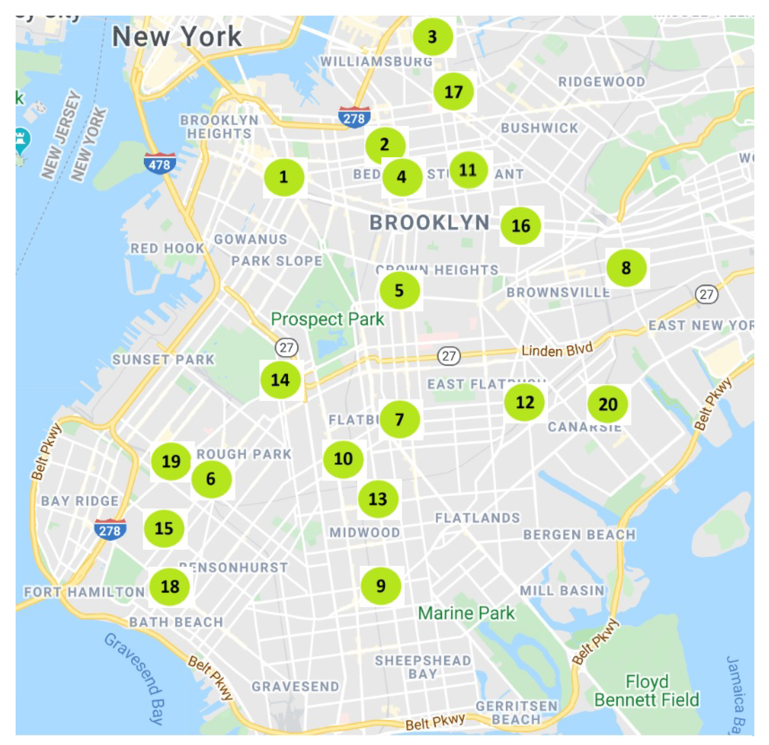Possible locations for mobile charging stations were randomly chosen so as to cover the entire area of the Brooklyn neighborhood in New York (see Figure 3).

Some of the parameters of the optimization problem are as follows: $C=(1,1,1,\cdots )$ (meaning, we can only assign a mobile charging station in node $j\in J_1$, and in node $j\in J_2$ we only assume there is one fixed charging station); g is obtained assuming that user charging requirements follow a normal distribution with mean 9 kW and a standard deviation of 1. The reason for choosing this distribution with these values of parameters can be found in [54] by Helmus and Van Den Hoed. They presented results related to the amount of charging of EV users and fitted the data using the normal distribution. Operating cost was assumed constant for all centers j, meaning $P_j=P=100$; the mean serving rate was ${\mu }_j\in [1.7\times {10}^{-6},1.77]$ for all $j\in J$ (unless otherwise stated) and $B_{max}=10$.

For different values of the parameters, we have different solutions. Depending on the charger capacity of the mobile charging station, we may need more or fewer charging stations.

Table 3. Results for different days for ${\omega }_U=150$ and 9:00–11:00 time period.

	Without Probability Constraints	b = 1, $\mathit{\beta }$ = 0.90	a = 1, $\mathit{\alpha }$ = 0.90	a = 1, b = 1, $\mathit{\gamma }$ = 0.90
	Monday
Solution	569.51	593.92	572.41	572.41
B	2	2	2	2
SoC${}_{max}$	119	132	132	132
SoC${}_{min}$	15	31	10	10
Location
mobile charging station	12, 15	5, 12	18, 20	18, 20
Location
fixed charging station	28, 55, 60, 61, 64	22, 55, 64	28, 52, 60, 61	28, 52, 60, 61
	Saturday
Solution	729.5	760.83	733.39	733.39
B	2	2	2	2
SoC${}_{max}$	142	149	142	142
SoC${}_{min}$	26	26	26	26
Location
mobile charging station	12, 18	5, 12	18, 20	18, 20
Location
fixed charging station	26, 52, 55, 61, 64	22, 49, 55, 62, 64	26, 52, 54, 61	26, 52, 54, 61

and

Table 4. Results for different days for ${\omega }_U=150$ and 12:00–15:00 time period.

	Without Probability Constraints	b = 1, $\mathit{\beta }$ = 0.90	a = 1, $\mathit{\alpha }$ = 0.90	a = 1, b = 1, $\mathit{\gamma }$ = 0.90
	Monday
Solution	460.38	482.12	541.62	541.62
B	1	1	2	2
SoC${}_{max}$	150	150	97	97
SoC${}_{min}$	9	39	9	9
mean(SoC)	52	77	52	52
Location
mobile charging station	9	5	15, 20	15, 20
Location
fixed charging station	48, 55, 60, 61, 64	51, 55, 64	42, 50, 60, 61	42, 50, 60, 61
	Saturday
Solution	356.57	368.31	356.98	356.98
B	1	1	1	1
SoC${}_{max}$	142	142	142	142
SoC${}_{min}$	21	21	25	25
mean(SoC)	55	55	73	73
Location
mobile charging station	13	12	13	13
Location
fixed charging station	55, 57, 59	49, 55, 62	57, 61	57, 61

shows the results obtained for Monday and Saturday, 9:00–11:00 and 12:00–15:00 time-frames for ${\omega }_U=150$.

Saturday and Monday between 9 o’clock and 11 o’clock, we need two mobile charging stations with or without considering probability constraints. However, their locations differ: for situations without probability constraints (locations 12 and 15) and with probability constraints (locations 5 and 12 for constraint $b=1$ and $\beta =0.90$, locations 18 and 20 for constraint $a=1,\alpha =0.90$ or $a=1,b=1,\gamma =0.90$). There may be cases wherein there is a need for more mobile charging stations just to make the service more efficient. On Monday, 12:00–15:00 time-frame, there is a need for a second mobile charging station, if the service operator decides to make sure it has at least one client with a probability of $0.9$. On Saturday, within the same time-frame we require one mobile charging station in location 12 or 13.

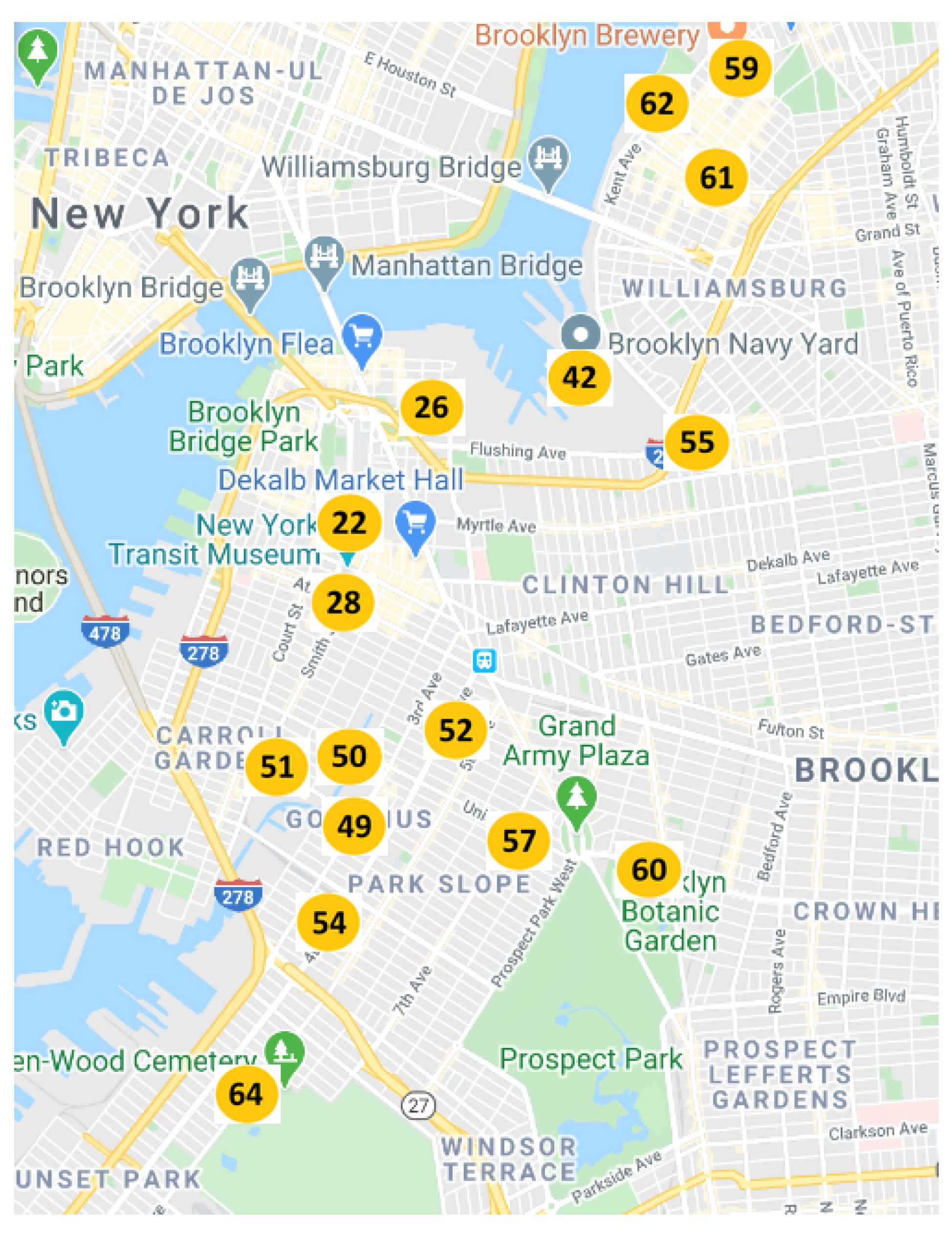
Different locations are obtained for different probability constraints. As the rate of charge improves, the mean service time decreases and the service is more efficient. The temporary locations of mobile charging stations obtained in Table 3 and Table 4 are in areas with no or few fixed charging stations. Most EVs are assigned to fixed charging stations when this is possible. Through computation optimization, EVS are assigned to fixed charging location in the northern part of Brooklyn (Table 3 and Table 4, Figure 4) and in this area no mobile charging station is located. It is possible that if in a area there is a sufficient fixed charging infrastructure, then there is no need for a mobile charging station. In this case, the mobile charging station can only act as a car attendant service.

6. Operational Metrics—Comparative Experiments

In the current operational mode, if we consider dynamic charging constraints, it may be that at some point on the journey to a new client, the mobile charging station may receive a new charge request [11,12], prolonging the service time for the new charge request.

In this section, we compare two operational modes of a mobile charging station considering some metrics of the service mobile charging station defined in [5]. These operational metrics quantify the performance of the operational mode of a mobile charging station. The first operational mode assumes moving the mobile station to where the EVs are located in order to recharge them, and the other one is the one introduced in this paper—the temporary location operational mode. For the first operational mode we assume a nearest-job-next (NJN) strategy, wherein the mobile station stays in the last location where it recharged an EV until a new charge request appears. Additionally, we assume that the mobile charging station has enough charger capacity (kW) to fulfill all charge requests in the service period considered.

One operational metric is the miss ratio index that measures the amount of charge requests that do not get to be satisfied within the service period. It is measured in percentage and it is defined as:

$$P_{miss}=\frac{N_{failed}}{N_{total}}\times 100$$

(33)

where $N_{total}$ represents the number of total requests received during service period, while $N_{failed}$ represents the number of requests that failed to be satisfied during the service period.

Another metric is the response time, which is defined as the time taken from when the EV sends out its charging request to the time when this request is completed. Another metric, which applies only for the second operational mode, is the queuing time, which is defined as the time taken from when the EV arrives to the location of the mobile charging station to the time the charging request is completed. These operational metrics are used to compare the two different operational modes mentioned. For each EV, we assume a charging time of 15 min while the service time is taken to be 9–13:00 on a Monday for NYC database. For moving operational mode, the initial location is in the center of the service area of Brooklyn.

In

Table 5. Operational metrics for moving and temporary location operational modes

Service Area	Response Time	(minutes)	Miss Ratio		Queuing Time (minutes)	Traveled Distance (km)
Operational mode	Moving	Location	Moving	Location	Location	Moving
${\lambda }_1$ = 0.00005
180 km${}^2$	179	105	0%	0%	15	864
100 km${}^2$	91	51	20%	20%	15	578
50 km${}^2$	37	34	0%	0%	15	192
${\lambda }_2$ = 0.0001
180 km${}^2$	181	84	6.25%	6.25%	24	1108
100 km${}^2$	74	54	0%	0%	17	533
50 km${}^2$	41	33	0%	0%	15	222
${\lambda }_3$ = 0.0002
180 km${}^2$	319	94	19%	0%	24	1276
100 km${}^2$	106	61	23%	23%	17	776
50 km${}^2$	60	36	18.75%	18.75%	17	509

we displayed some empirical results obtained through simulations. Charging requests appear following a Poisson process of parameter $\lambda$, while we consider the depot to be in the center of service area. The depot is the initial location of mobile charging station in moving operational mode, and it is the temporary location in the new operational mode. Different dimensions of the service area are taken into account.

Miss ratios in both strategies are similar; however, the miss ratios of temporary location operational are always smaller or equal to those of moving operational mode. We cannot say the same about the response times of the service, which are significantly influenced by the dimensions of the service area, with the response times of moving operational mode being always greater than those for temporary location strategy (large differences can be observed). As the intensity of charge requests $\lambda$ decreases along with a smaller service area (around 50 km${}^2$), the response times of the two strategies are comparable and we may be able to choose one strategy or the other. However, for moving operational mode, we have the problem of travel distance that increases the cost of operations of a mobile charging station. The travel distance can be substantial even for a small service area.

Results obtained through the NYC database, as shown in the previous section, also suggest that the temporary location operational mode is the better one. Our comparative experiments showed a 36% miss ratio for the moving operational mode (initial location is the center of Brooklyn), while for our mode of operation the miss ratio is only 9% (temporary location is also the center of Brooklyn). This is due to the fact that as the mobile charging station stations and charges EVs, the time it should take the mobile station to reach each EV is taken over by each EV. Therefore, the service becomes more efficient, thereby allowing the mobile charging station to fulfill more charge requests.

As for the response time, the mean response time for the first mentioned operational mode is 57 min (without the EVs that could not be charged within the service period considered) or an hour and 43 min (considering all charge requests completed). Concerning our temporary location operational mode, the mean response time is 40 min, while the mean queuing time spend by an EV at the location of the mobile charging station is 21 min. Moreover, the total distance needed for the mobile charging station to fulfill all requests in the moving operational mode is 61.94 km or 1 h and 36 min of driving. Furthermore, the travel distance of a mobile charging station may vary due to traffic constraints, weather and temperature [11].

One advantage of the temporary location strategy is the reduced response time of the service. In a survey conducted in 2016 [55] the authors evaluated the different drawbacks that can occur by owning an EV. The results speak by themselves: EV’s drivers are willing to make a detour to recharge, but they strongly reject waiting times. Since, for the moving operational time we have such a long period of waiting, this can be a serious issue for EV drivers. Thus, temporary location of mobile charging station may be preferable to moving the mobile charging station from one place to another. Moreover, because EV’s drivers do not reject making a detour to recharge, this is an argument in favor of a temporary location strategy.

7. Conclusions

In this paper, a new operational mode for a mobile charging station which assumes temporary locations in some possible places for certain periods of time is introduced. We formulate this problem as a location-allocation problem considering queuing constraints (at most b clients and/or at least a clients).

Our contributions in this paper are summarized as follows:

• We formulated a nonlinear optimization problem and an equivalent mixed-linear optimization problem for optimal temporary location of a mobile charging station.
• We obtained new probability-queuing constraints, considering at least a clients in the queue and/or at most b clients in the queue.
• We compared two operational modes for a mobile charging station.

The key findings of our work are:

• Different temporary locations are obtained for different probability constraints and days of the week.
• The locations obtained are in areas with no or few fixed charging stations.
• The temporary location operational mode compared to moving operational mode has a smaller mean response time.
• Travel distance is an issue in moving operational mode, increasing operational costs, a problem that does not arise in the temporary location strategy.

Of course, these results have been obtained assuming a charging time of less than 30 min, which may be very realistic for the next few years. Future research will also take into account other practical constraints that may be included in the implementation of the charging station based on a fuel cell hybrid power supply [56,57] with appropriate control in current and voltage [58,59]. This paper is a basis for future directions, such as:

• The development of a new strategy in different urban areas to install predictive charging stations;
• Another study in which we intend to use installed charging stations and gather data on the number of cars, the flow of cars in certain time periods and driver behavior given by GPS data;
• A study for increasing the percentage of renewable energy that supplies charging stations; for example, a charging station with PV on the roof;
• Uncertainty analysis with fuzzy intervals;
• Extending the work by considering Markov dependence hypothesis.