Resonance Enhancement by Suitably Chosen Frequency Detuning

Abstract

The theory of exact resonances (kinematics and dynamics) is well developed while even the very concept of detuned resonance is ambiguous and only studies of their kinematic characteristics (that is, those not depending on time) are available in the literature. In this paper, we report novel effects enforced by the resonance detuning on solutions of the dynamical system describing interactions of three spherical planetary waves. We establish that the energy variation range can significantly exceed the range of the exact resonance for suitably chosen values of the detuning. The asymmetry of system’s solutions with respect to the sign of the detuning parameter is demonstrated. Finally, a non-monotonic dependence of the energy oscillation period with respect to detuning magnitude is discovered. These results have direct implications in physics of atmosphere, e.g., for prediction of weather extremes in the Northern Hemisphere midlatitudes (Proc. Nat. Acad. Sci. USA 2016, 133(25), 6862–6867). Moreover, similar study can be conducted for a generic three-wave system taken in the Hamiltonian form which makes our results applicable for an arbitrary Hamiltonian three-wave system met in climate prediction theory, geophysical fluid dynamics, plasma physics, etc.

1. Introduction

Numerous natural phenomena exhibit linear and nonlinear resonances. In many technical cases occurrence of resonance must to be avoided, the widely known Tacoma Bridge dramatic collapse being an example for this. In other cases, the goal is to approach the state of exact resonance, by reducing resonance detuning, in order to increase the efficiency of a process or device. To give a notion of linear resonance in physics, we consider a linear oscillator (a pendulum in mechanical problems or a wave in the form of the Fourier harmonics in fluid dynamics problems), driven by a small force. We say, that the resonance occurs, if the eigenfrequency $\omega$ of a system coincides with the frequency of the driving force $\mathsf{\Omega }$. In this case, for small enough resonance detuning, $|\mathsf{\Omega }-\omega |>0$, the amplitude of the linear oscillator becomes smaller with increasing detuning.

The simplest case of nonlinear resonance is a set of three waves $A_j{\mathrm{e}}^{\mathrm{i}({\mathit{k}}_j{\mathit{x}}_j-{\omega }_{j}t)}$ fulfilling exact resonance conditions of the following form

$$\begin{array}{c}{\omega }_1\pm {\omega }_2\pm {\omega }_3=0,\end{array}$$

(1)

$$\begin{array}{c}\hfill {\mathit{k}}_1\pm {\mathit{k}}_2\pm {\mathit{k}}_3=0,\end{array}$$

(2)

where ${\mathit{k}}_j\in {\mathbb{Z}}^2$, ${\omega }_j=\omega ({\mathit{k}}_j)$ are the wave vectors and frequencies respectively. Notice that this definition differs substantially from the mathematical notion of resonance which makes use only of the first Equation (1), see e.g., [1]. Moreover, in mathematical definition frequencies ${\omega }_j$ are variables, not functions, and the properties of corresponding dynamical systems are characterized by the ratios of frequencies. This difference is very important and, in particular, shows that exact mathematical results available in this area cannot be directly used in solving a physical problem. The fact is that in the Hamiltonian system Equations (1) and (2) do present the laws of energy and momentum conservation respectively, and must both be satisfied.

We do not aim to describe all the possible manifestations of the resonance phenomenon in various natural systems, and confine ourselves to a brief introduction to the classical Wave Turbulence Theory (WTT), which assumes resonance as the main acting mechanism in a weakly nonlinear wave system. In the frame of the WTT, a wave system is governed by a weakly nonlinear dispersive partial differential equation (PDE) whose linear part has solutions in the form of Fourier modes $Aexp(\mathbf{k}\mathbf{x}-\omega t)$ where $\mathbf{x}$ and t are space and time variables consequently, $\mathbf{k}$ is wave vector, and wave frequency $\omega$ is a function of the wave vector, $\omega =\omega (\mathbf{k})$, it is also called dispersion function. The nonlinear part of the PDE should be small, which is achieved by introducing a small parameter $\epsilon$, $0<\epsilon \ll 1$, the physical meaning of which changes from one wave system to another. For instance, in the case of surface water waves, the wave steepness is usually regarded as a suitable small parameter while for the atmospheric planetary waves $\epsilon$ can be taken as the ratio of phase and group velocities. The waves are said to interact resonantly (that is, to form an exact resonance) if resonant conditions given in Equations (1) and (2) are satisfied.

Under a set of assumptions, time evolution of weakly nonlinear systems is described by the waves taking part in exact resonant interactions, while non-resonant waves are neglected in a sense that their energies can be regarded as constant (of course, only at some specific time scale depending on $\epsilon$). Depending on whether the system is considered in a bounded area (the so-called resonators) or in an infinite domain, the theory gives two types of predictions. In the first case, small clusters of resonantly interacting waves are formed; the waves exchange the energy within a cluster, and there is no energy flow among the clusters. Accordingly, the original PDE can be reduced to a few finite systems of ordinary differential equations (ODE) which can be solved independently (discrete WTT [2,3]). On the other hand, under a set of statistical assumptions, the original PDE can be reduced (at some longer time scale) to a wave kinetic equation whose stationary solution gives a stationary distribution of energy over scales in the Fourier space (kinetic WTT [4,5]). The WTT is widely used for explaining the various effects that arise in real physical, technical, biological, economic, medical and other problems, numerous examples of applications can be found in [6].

The notion of resonance enhancement via frequency detuning, as the title of this manuscript says, contradicts what we would expect from our physical intuition. However, there exists a simple qualitative explanation for that. Indeed, our intuition comes from a linear pendulum

$$\ddot{x}+{\omega }^{2}x=0,$$

(3)

taken usually as a model for a linear wave, and a resonance is regarded due to an action of an external force. On the other hand, the dynamical system for three-wave resonance can be transformed into the Mathieu equation which describes a particular case of the motion of an elastic pendulum

$$\ddot{x}+[{\omega }_{\mathrm{pen}}^2-\lambda cos({\omega }_{\mathrm{spr}})]x=0,$$

(4)

where ${\omega }_{\mathrm{pen}}$ and ${\omega }_{\mathrm{str}}$ are frequencies of pendulum- and spring-like motions ([3], Chapter 5). Regarding resonance detuning $\widetilde{\Delta \omega }$ as a frequency of an external force for Equation (4), our findings can be understood in the following way. The detuned three-wave system has the maximal range of the energy amplitudes variation when the elastic pendulum interacts resonantly with the external forcing. Detailed study of this effect can be performed, using the approach developed in [7] for an elastic pendulum subject to the external force.

Drawn from the resonance conditions provided in Equations (1) and (2), resonance detuning in the nonlinear case can be defined in a number of ways, e.g., as a phase detuning [8], or frequency detuning [9,10,11]. The frequency detuning, used in the present paper, is defined as

$${\omega }_1+{\omega }_2-{\omega }_3=\widetilde{\Delta \omega },\left|\widetilde{\Delta \omega }\right|\ll \underset{j=1,2,3}{min}\left\{{\omega }_j\right\},$$

(5)

and detuned resonances have to satisfy conditions given in Equations (5) and (2). Exact and detuned resonances may appear in the same wave system, at different time scales or under slightly different conditions. For instance, Zakharov’s kinetic equation describes time evolution of surface water waves and takes into account only exact resonances [5], while various generalized wave kinetic equations include detuned resonances for describing additional effects, e.g., wave field evolution under the action of wind blasts [12]. Another example is given by exact resonances of the atmospheric planetary waves which are governed by the Barotropic Vorticity Equation (BVE) and describe intra-seasonal oscillations in the Earth’s atmosphere [13], with periods 30 to 60 days. On the other hand, detuned resonances of the same type of waves are used to characterize regional summer weather extremes in the Northern Hemisphere [14,15].

From mathematical point of view, the study of exact resonances in the frame of WTT is conducted along the following lines. (I) Original nonlinear PDE taken with suitable boundary conditions yields the form of dispersion function $\omega =\omega (\mathbf{k})$. (II) Exact solutions of Equations (1) and (2) can be found (for big classes of physically relevant dispersion functions) by specially developed methods [16,17,18], and corresponding resonance clusters can be constructed. (III) For each cluster a unique dynamical system of nonlinear ODEs can be deduced and solved analytically or numerically. (IV) Alternatively to (III), an averaging statistical procedure is used over the entire set of dynamical systems yielding kinetic (meaning stationary) regime.

Unlike exact resonances, the theory of detuned resonances does not yet exist and their properties common to various nonlinear systems are not known. Existing studies are limited to kinematics, i.e., a study of the structure of many quasi-resonances depending on the magnitude of the detuning. Moreover, the structure under consideration is presented in a form that allows neither to restore corresponding dynamical system, nor to deduce any dynamical characteristics of a detuned resonance [10]:

In order to better understand these issues, we believe that it is important to move beyond the kinematic picture of resonance broadening and attempt to devise methods of studying these effects dynamically.

Generally, in the physical literature, the prevailing opinion is that bigger detuning results in smaller variation of amplitudes and that dynamics of a detuned triad is similar to a resonant one, e.g., [19]. To study detuned resonances in a specific wave system, the amplitudes are used, calculated not from dynamic equations, but from specially processed measurement’s data [15].

In this paper we study for the first time the effects of frequency detuning in Equation (1) by means of the numerical simulation with corresponding dynamical system. As an example we take a resonant triad of atmospheric planetary waves from [13]. For the readers convenience we begin in the Section 2 with barotropic vorticity equation and deduce from it corresponding dynamical system. The system of model equations is discribed in Section 3. Numerical results for the amplitudes and the phase space are presented and analyzed in the Section 4 and the Section 5 correspondingly. Brief discussion concludes the paper.

2. Barotropic Vorticity Equation

We have chosen the Barotropic Vorticity Equation (BVE) on a sphere for demonstrating the very procedure of deducing dynamical equations for resonantly interacting waves from the initial evolution equation in partial derivatives. It is also known under the names Charney, Obukhov–Blinova, Hasegawa–Mima equation and describes large motion of Rossby (also called planetary or drift) waves in the planets atmospheres, oceans, laboratory and cosmic plasmas, etc. The BVE in its simplest form reads

$$\frac{\partial {\nabla }^2\zeta }{\partial t}+2\frac{\partial \zeta }{\partial \lambda }+\epsilon J(\zeta ,{\nabla }^2\zeta )=0$$

(6)

with small parameter $\epsilon$, $0<\epsilon \ll 1$. Here the Laplacian and Jacobian are given as

$${\nabla }^2\psi =\frac{{\partial }^2\zeta }{\partial {\phi }^2}+\frac{1}{{cos}^2\phi }\frac{{\partial }^2\zeta }{\partial {\lambda }^2}-tan\phi \frac{\partial \zeta }{\partial \phi },$$

(7)

$$J(a,b)=\frac{1}{cos\phi }\left(\frac{\partial a}{\partial \lambda }\frac{\partial b}{\partial \phi }-\frac{\partial a}{\partial \phi }\frac{\partial b}{\partial \lambda }\right)$$

(8)

and the linear part of spherical BVE has wave solutions in the form

$$A{P}_n^m(sin\phi )exp\left(\mathrm{i}\left[m\lambda +\frac{2m\beta }{n(n+1)}t\right]\right)$$

(9)

with latitude $\phi$, $-\pi /2\le \phi \le \pi /2$, and the longitude $\lambda$, $0\le \lambda \le 2\pi$. Here A is constant wave amplitude, $\omega =-2\beta m/[n(n+1)]$, $P_n^m(sin\phi )$ is the associated Legendre function of degree n and order $m$, and $\beta$ is dimensional derivative of the Coriolis parameter with respect to the latitude. We use physical notation for the Laplacian, ${\nabla }^2$, instead of mathematical Δ in order to avoid a possible confusion with the detuning $\Delta$.

For studying resonant interactions of spherical planetary waves, we (a) assume that amplitudes $A_{\mathbf{k}}=A_{\mathbf{k}}(T)$ are slowly changing functions on $T=\epsilon t$, and (b) search for a solution as a series on the powers of the small parameter $\epsilon$:

$$\zeta ={\zeta }_0(\lambda ,\phi ,t,T)+\epsilon {\zeta }_1(\lambda ,\phi ,t,T)+{\epsilon }^2{\zeta }_2(\lambda ,\phi ,t,T)+\dots$$

(10)

in the form of a sum of three linear waves:

$${\zeta }_0(\lambda ,\phi ,t,T)=\sum _{k=1}^3{A}_k(T)P^{(\mathbf{k})}cos{\theta }_{\mathbf{k}},$$

(11)

where notations $P^{(\mathbf{k})}=P_{n_{\mathbf{k}}}^{m_{\mathbf{k}}}(sin\phi )$ and ${\theta }_{\mathbf{k}}=[m_{\mathbf{k}}\lambda -\omega (\mathbf{k})t]$ are used.

Substituting the ansatz (10) in Equation (6) and combining the terms with the same power of small parameter $\epsilon$, we get the coefficient in front of the term with ${\epsilon }^0$ of the form

$$\frac{\partial }{\partial t}{\nabla }^2{\zeta }_0+2\frac{\partial }{\partial x}{\zeta }_0=0;$$

(12)

the coefficient in front of the term with ${\epsilon }^1$ of the form

$$\frac{\partial }{\partial t}{\nabla }^2{\zeta }_1+2\frac{\partial }{\partial \lambda }{\zeta }_1=-J({\zeta }_0,{\nabla }^2{\zeta }_0)-\frac{\partial }{\partial T}{\nabla }^2{\zeta }_0,$$

(13)

and so on. We fix resonance condition in the form ${\theta }_{{\mathit{k}}_1}+{\theta }_{{\mathit{k}}_2}={\theta }_{{\mathit{k}}_3}$, use the orthogonality of the functions ${\psi }_1$ and ${\psi }_0$ in order to avoid an unbounded growth of left-hand side in Equation (13), and integrate all over the sphere $(\lambda ,\phi )$ with $t\to \infty$. In this way we remove all variables but slow time T and deduce two dynamical equations

$$\begin{array}{c}{N}_3{\dot{A}}_3=2\mathrm{i}Z(N_2-N_1)A_1{A}_2,\end{array}$$

(14)

$$\begin{array}{c}{N}_3{\dot{A}}_3^{*}=-2\mathrm{i}Z(N_2-N_1)A_1^{*}{A}_2^{*},\end{array}$$

(15)

where $N_j=n_j(n_j+1)$, $j=1,2,3$ and interaction coefficient Z is a number computed as

$$Z={\int }_{-\pi /2}^{\pi /2}\left[m_2{P}^{(2)}\frac{\mathrm{d}}{\mathrm{d}\phi }{P}^{(1)}-m_1{P}^{(1)}\frac{\mathrm{d}}{\mathrm{d}\phi }{P}^{(2)}\right]\frac{\mathrm{d}}{\mathrm{d}\phi }{P}^{(3)}\mathrm{d}\phi .$$

(16)

Change of signs in Equations (1) and (2) yields another form of resonance conditions and the use of same procedure gives dynamical equations for ${\dot{A}}_1$ and ${\dot{A}}_2$. The final dynamical system for exact three wave resonance reads

$$\begin{array}{c}{N}_1{\dot{A}}_1=-2\mathrm{i}Z(N_2-N_3)A_3{A}_2^{*},\end{array}$$

(17)

$$\begin{array}{c}{N}_2{\dot{A}}_2=-2\mathrm{i}Z(N_3-N_1)A_1^{*}{A}_3,\end{array}$$

(18)

$$\begin{array}{c}{N}_3{\dot{A}}_3=2\mathrm{i}Z(N_1-N_2)A_1{A}_2\end{array}$$

(19)

(and their complex conjugate equations) where the dot denotes differentiation with respect to the slow time $T=\epsilon t$. We omit here details of this tedious but straightforward calculations, details of the implementation of this procedure in Mathematica can be found in [20]. This system is has three integrals of motion is explicitly integrable in Jacobian elliptic functions.

At the end of this Section, we would like to make a remark. The dynamical system for three resonantly interacting waves is Hamiltonian system. It has canonical form

$${\dot{B}}_1=V_3^{1,2}{B}_2^{*}{B}_3,{\dot{B}}_2=V_3^{1,2}{B}_1^{*}{B}_3,{\dot{B}}_3=-V_3^{1,2}{B}_1{B}_2,$$

(20)

which looks more simple than Equations (17)–(19) and is valid for arbitrary three-wave Hamiltonian system. However, the canonical variables $B_j$ are not physical entities and interpretation of any theoretical results obtained for Equations (20) should include a nontrivial task of coming back to physical variables. That is the reason why our numerical simulations presented below were conducted for the equations written in terms of amplitudes and phases, thus allowing direct physical interpretation.

3. Model Equations

The dynamical system for detuned resonance of three complex-valued amplitudes $A_i$, $i=1,2,3$ reads

$$\begin{array}{c}{N}_1\dot{A_1}=-2\mathrm{i}Z(N_2-N_3)A_2^{*}{A}_3{\mathrm{e}}^{-\mathrm{i}\Delta \omega T},\end{array}$$

(21)

$$\begin{array}{c}{N}_2\dot{A_2}=-2\mathrm{i}Z(N_3-N_1)A_1^{*}{A}_3{\mathrm{e}}^{-\mathrm{i}\Delta \omega T},\end{array}$$

(22)

$$\begin{array}{c}\hfill N_3\dot{A_3}=2\mathrm{i}Z(N_1-N_2)A_1{A}_2{\mathrm{e}}^{\mathrm{i}\Delta \omega T},\end{array}$$

(23)

(and their complex conjugate equations) where the dot denotes differentiation with respect to the slow time $T=t/\epsilon$, $\Delta \omega :=\widetilde{\Delta \omega }/\epsilon$, $\epsilon$ being a small parameter. The dynamical system for exact resonance is obtained by setting $\Delta \omega \equiv 0$. It can be rewritten in amplitude/phase variables as

$$\begin{array}{c}{N}_1\dot{C_1}=-2Z(N_2-N_3)C_2{C}_{3}sin\psi ,\end{array}$$

(24)

$$\begin{array}{c}{N}_2\dot{C_2}=-2Z(N_3-N_1)C_1{C}_{3}sin\psi ,\end{array}$$

(25)

$$\begin{array}{c}{N}_3\dot{C_3}=-2Z(N_1-N_2)C_1{C}_{2}sin\psi ,\end{array}$$

(26)

$$\begin{array}{c}\dot{\psi }=\Delta \omega -2Z{C}_1{C}_2{C}_3(\frac{N_2-N_3}{N_1}{C}_1^{-2}+\end{array}$$

(27)

$$\begin{array}{c}\frac{N_3-N_1}{N_2}{C}_2^{-2}+\frac{N_1-N_2}{N_3}{C}_3^{-2})cos\psi ,\end{array}$$

(28)

where $C_i(T)=\left|A_i(T)\right|$ is the real amplitude, $\psi :={\theta }_1+{\theta }_2-{\theta }_3$ is the dynamical phase and ${\theta }_i(T)=arg{A}_i(T)$. In what follows, we will focus on the evolution of the energy of the high-frequency mode ${\mathcal{E}}_3(T)$.

4. Amplitudes

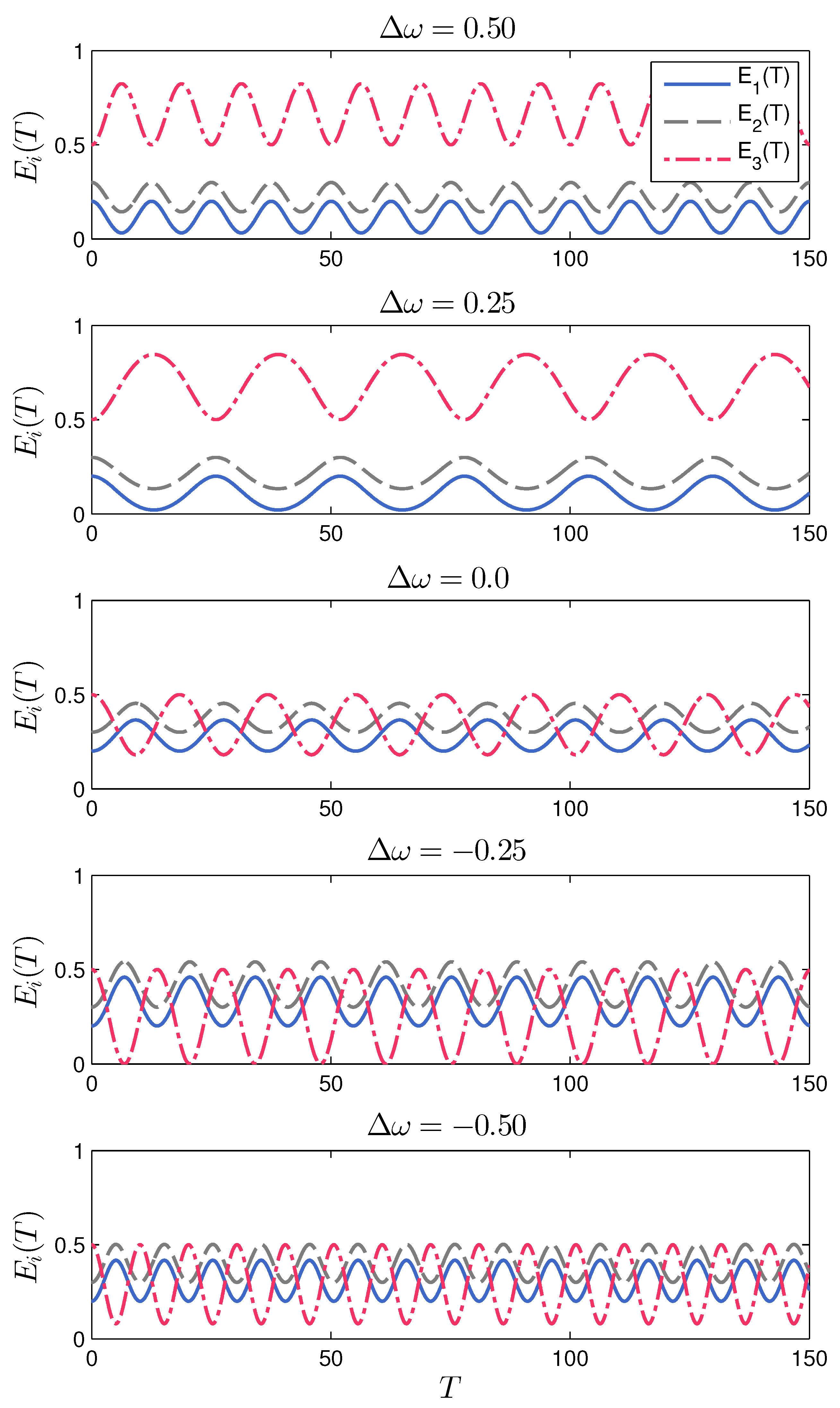
For all numerical simulations we used the Matlab^TM software along with its standard ODE Suite [21]. In particular, the standard ode45 solver was employed with stringent error tolerance settings. In Figure 1 we show the energy evolution in the resonant triad given in Table 1 for several values of the frequency detuning $\Delta \omega =\widetilde{\Delta \omega }/\epsilon \in [-\frac{1}{2},\frac{1}{2}]$; e.g., in geophysical applications $\epsilon \sim \mathcal{O}({10}^{-2})$. From these graphs it can be seen that the period $\tau$ and the range of the energy variation, defined as

$$\Delta \mathcal{E}(\Delta \omega ):=\frac{1}{2}\left(\underset{t}{max}\mathcal{E}-\underset{t}{min}\mathcal{E}\right),$$

(29)

are non-monotonic functions of the detuning $\Delta \omega$.

Figure 1. Energy evolution in the triad given in Table 1, for different values of the detuning $\Delta \omega$.

Table 1. Physical parameters used in numerical simulations.

Parameter	Value
Resonant wave vectors, $[m_j,n_j]$	$[4,12]$, $[5,14]$, $[9,13]$
Resonant frequencies, $2m_j/n_j(n_j+1)$	$0.0513$, $0.0476$, $0.0989$
Resonant triad parameters, $N_j$	156, 210, 182
Interaction coefficient, Z	$7.82$
Initial energy distribution (a), %	20%, 30%, 50%
Initial energy distribution (b), %	40%, 40%, 20%
Initial dynamical phase, $\psi$	0.0

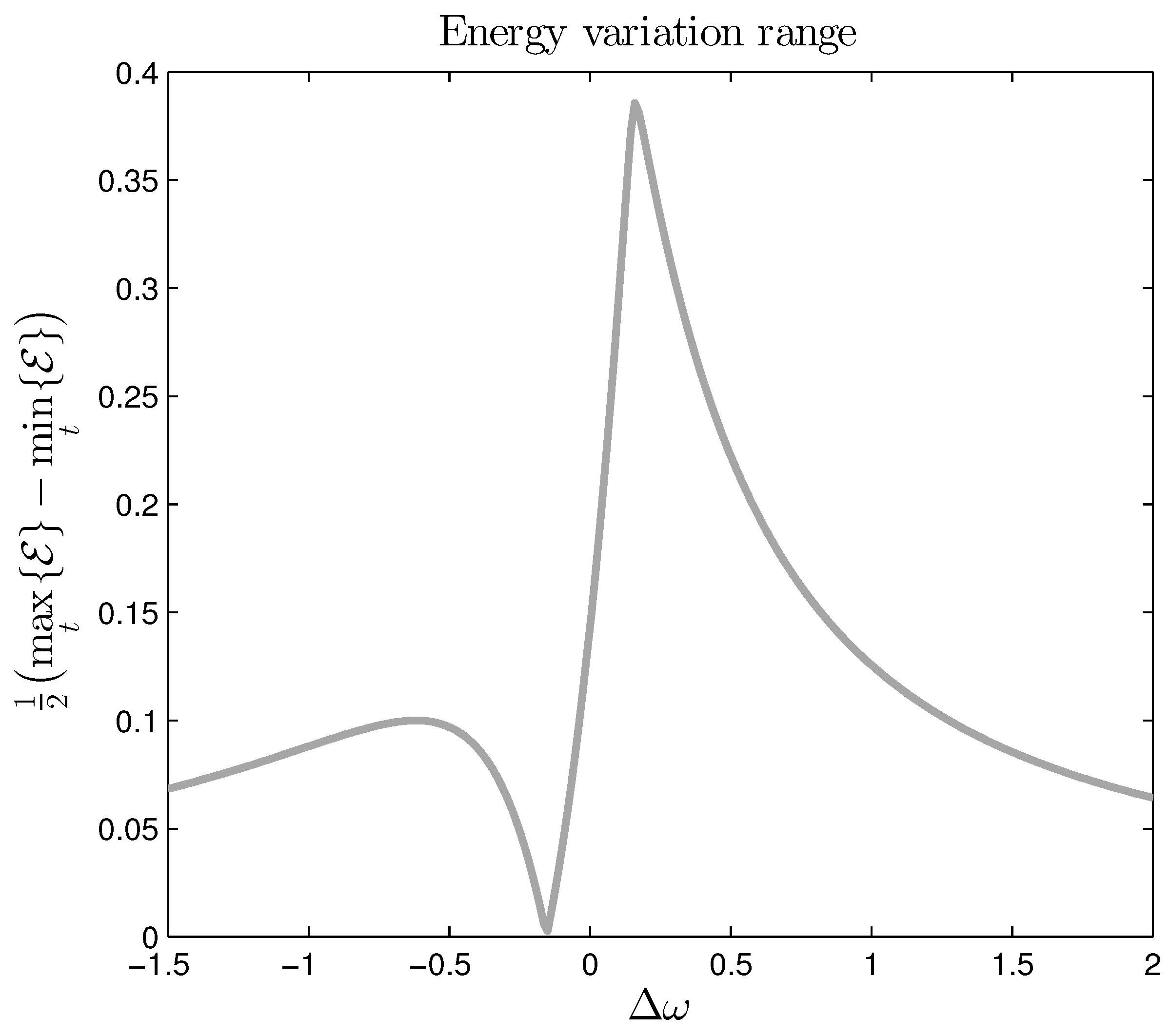
A graph showing the characteristics of the dependency of the energy variation range $\Delta \mathcal{E}(\Delta \omega )$ on the frequency detuning $\Delta \omega$ is shown in Figure 2. This particular curve was computed for parameters given in Table 1. The graph can conveniently be divided into the five regions which are separated by particular values of the frequency detuning $\Delta \omega$: $\Delta {\omega }_{max}^{(1,2)}$ correspond to local maxima, $\Delta {\omega }_{\mathrm{st}}$ is the position of the local minimum, and $\Delta \omega =0$ corresponds to exact resonance. So, the regions are:

Figure 2. Typical dependency of the energy variation range $\Delta \mathcal{E}$ on the frequency detuning $\Delta \omega$ for the case when the high frequency mode ${\omega }_3$ has the maximal energy (initial condition from Table 1). The vertical red dashed line shows the location of $\Delta {\omega }_{max}^{(1)}$, while the vertical black solid line shows the location of $\Delta {\omega }_{max}^{(2)}$. Finally, the blue dash-dotted line shows the amplitude obtained the exact resonance.

(I)

$\Delta \omega \in \left(-\infty ,\Delta {\omega }_{max}^{(1)}\right]$;

(II)

$\Delta \omega \in \left(\Delta {\omega }_{max}^{(1)},min\{0,\Delta {\omega }_{\mathrm{st}}\}\right]$;

(III)

$\Delta \omega \in \left(min\{0,\Delta {\omega }_{\mathrm{st}}\},max\{0,\Delta {\omega }_{\mathrm{st}}\}\right]$;

(IV)

$\Delta \omega \in \left(\Delta {\omega }_{\mathrm{st}},\Delta {\omega }_{max}^{(2)}\right]$;

(V)

$\Delta \omega \in \left(\Delta {\omega }_{max}^{(2)},+\infty \right)$.

The reason to regard these regions separately is that the main characteristics (i.e., energy variation $\Delta \mathcal{E}$, energy oscillation period $\tau$ and the phase variation $\Delta \psi$) behave differently in each region. Our findings are summarized in Table 2, where all the quantities $\mathcal{E}$, $\tau$ and $\psi$ are followed by ± sign denoting the their variation in the region (+: increase, −: decrease). The first column corresponds to the direction of increasing values of $\Delta \omega \in (-\infty \to +\infty )$, while the second column corresponds to the opposite direction $\Delta \omega \in (-\infty \leftarrow +\infty )$.

Table 2. Behaviour of physical parameters $\Delta \mathcal{E}$, $\tau$ and $\psi$ in different regions.

Region/Range	⟶	⟵
(I)	$\Delta \mathcal{E}+$, $\tau +$, $\Delta \psi -$	$\Delta \mathcal{E}-$, $\tau -$, $\Delta \psi +$
(II)	$\Delta \mathcal{E}-$, $\tau +$, $\Delta \psi -$	$\Delta \mathcal{E}+$, $\tau -$, $\Delta \psi +$
(III)	$\Delta \mathcal{E}-$, $\tau +$, $\Delta \psi -$	$\Delta \mathcal{E}+$, $\tau -$, $\Delta \psi +$
(IV)	$\Delta \mathcal{E}+$, $\tau -$, $\Delta \psi +$	$\Delta \mathcal{E}-$, $\tau +$, $\Delta \psi -$
(V)	$\Delta \mathcal{E}-$, $\tau -$, $\Delta \psi +$	$\Delta \mathcal{E}+$, $\tau +$, $\Delta \psi -$

The most interesting observation is, that the energy variation range during the system evolution can be significantly larger for a suitable choice of the detuning $\Delta \omega \ne 0$ compared to the exact resonance case $\Delta \omega =0$. There are two values of which provide significant amplifications to $\Delta \mathcal{E}$. On Figure 2 the global maximum is located on the left of $\Delta {\omega }_{\mathrm{st}}$, while on Figure 3 it is on the right of $\Delta {\omega }_{\mathrm{st}}$. These two cases differ only by the initial energy distribution among the triad modes (see Table 1, initial conditions (a) & (b)).

Figure 3. Typical dependence of the energy variation range $\Delta \mathcal{E}$ on the frequency detuning $\Delta \omega$ for the case when the high frequency mode ${\omega }_3$ has the lowest energy (initial condition from Table 1).

Similar computations have been performed for other resonant triads and the qualitative behavior of the energy variation has always been similar to Figure 2 and Figure 3. Namely, the global maximum is located on the left of $\Delta {\omega }_{\mathrm{st}}$ when the high frequency mode ${\omega }_3$ contains initially most of the energy, and to the right of $\Delta {\omega }_{\mathrm{st}}$ in the opposite case.

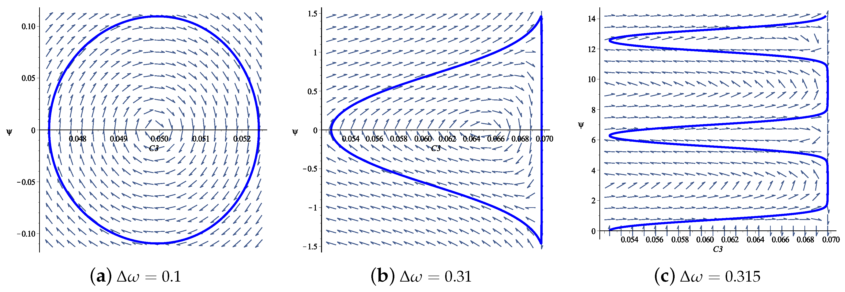
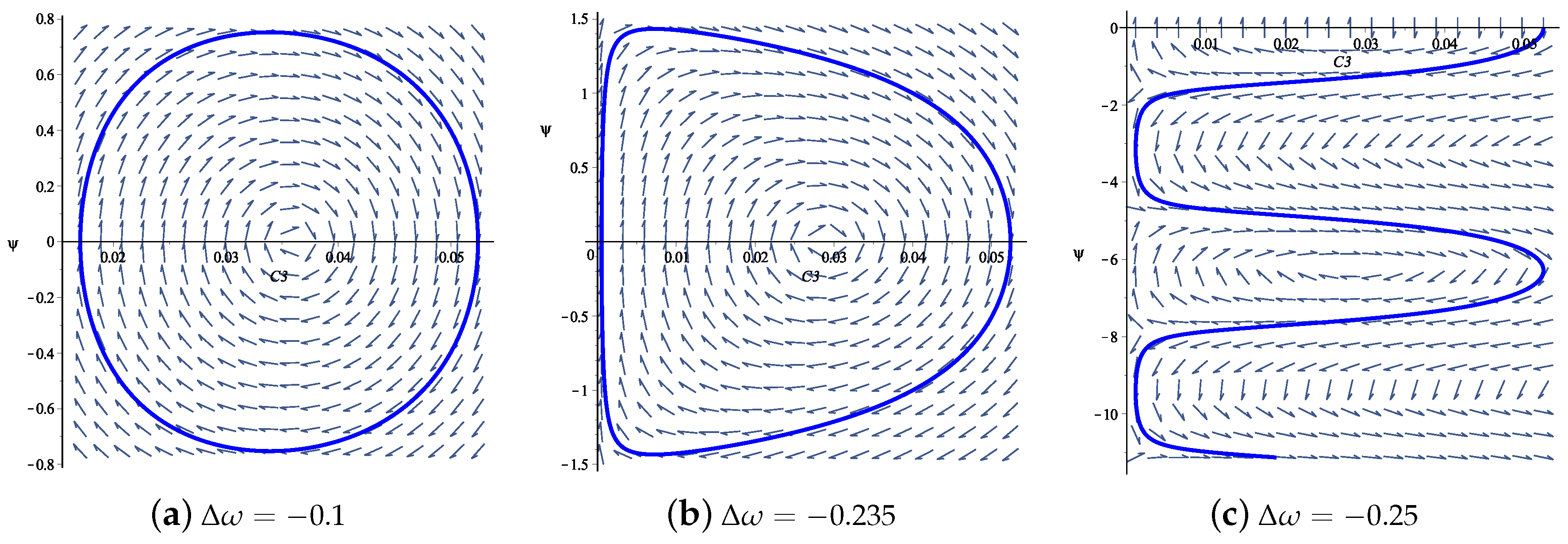
It is important to stress that the energy variation $\Delta \mathcal{E}(\Delta \omega )$ at the global maximum $\Delta {\omega }_{max}^{(\mathrm{g})}$ is always significantly higher than at the point of exact resonance, i.e., $\Delta \mathcal{E}(\Delta {\omega }_{max}^{(\mathrm{g})})>\Delta \mathcal{E}(0)$. The highest ratio $\Delta \mathcal{E}(\Delta \omega )/\Delta \mathcal{E}(0)$ is attained when the local minimum $\Delta {\omega }_{\mathrm{st}}$ coincides with the point of exact resonance. In this case we can find a $\Delta \omega$ that the amplification $\Delta \mathcal{E}(\Delta \omega )/\Delta \mathcal{E}(0)$ is of at least one order of magnitude. A simple phase space analysis allows to locate the local minimum.

5. Phase Space Analysis

The phase space analysis was performed with Maple^TM software. On Figure 4, Figure 5 and Figure 6 we depict the typical phase portraits of the dynamical system of Equations (24)–(28) in phase-amplitude variables. For illustration we choose the triad given in Table 1 with the initial energy distribution (a). In these pictures we represent the high-frequency mode $C_3$ on the horizontal axis, while the dynamical phase $\psi$ is on the vertical.

Figure 4. Phase portraits of the dynamical system of Equations (24)–(28) in $(C_3,\psi )$ variables for the triad from Table 1 (case (a)). Positive increasing detuning.

Figure 5. Phase portraits of the dynamical system of Equations (24)–(28) in $(C_3,\psi )$ variables for the triad from Table 1. Negative decreasing detuning.

Figure 6. Simultaneous plot of two phase portraits and integral curves for the detunings $\Delta \omega =\pm 0.1$ shown at Figure 4a and Figure 5a correspondingly.

The main finding is a pronounced asymmetry between the phase portraits for positive and negative values of the detuning $\Delta \omega$: the position of the stationary point right on the horizontal axis $C_3$ (there are other stationary points for $\psi \ne 0$) is very different; the shape of the periodic orbit differs (see Figure 4b and Figure 5b); the transition from closed to snake-like integral curves takes place for different values of $|\Delta \omega |$, e.g., $\approx 0.31$ on Figure 4c and $\approx -0.24$ on Figure 5c; the shape of the integral curves is different; the phase portraits look alike, but differ in size by one order of magnitude. In order to demonstrate how big this difference is for opposite values of $\Delta \omega$ we depicted on the same Figure 6 the periodic cycles from Figure 4a and Figure 5a.

A simple phase space analysis reveals the reason for the presence of a local minimum of $\Delta \mathcal{E}$ in Figure 2 and Figure 3. Indeed, it can happen that the initial conditions coincide with the system equilibrium point, which depends on $\Delta {\omega }_{\mathrm{st}}$.

6. Conclusions

In this paper we studied dynamics of three spherical planetary waves under the action of a small frequency detuning. For our numerical computations we used two different forms of corresponding dynamical system—(a) one with complex amplitudes being variables (suitable for immediate interpretation of the results in terms of energies), and (b) another—in the amplitude-phase presentation (more suitable for studying the phase space).

It was demonstrated that the introduction of frequency detuning significantly enriches the dynamics of a three-wave resonance system. Moreover, the effects of detuning are highly nonlinear and highly non-monotonic with respect to the detuning parameter. The main findings of this study are outlined hereinbelow:

• The range of values of frequency detuning $\Delta \omega$ can most conveniently be divided into five regions of different behaviour, not all of them present in any case. The behavior of the main parameters of System of Equations (24)–(28) over those five regions is summarized in Table 2.
• The amplitude of energy variation Equation (29) in a triad with suitably chosen detuning ($\Delta \omega \ne 0$) can be significantly higher than in the case of exact resonance, i.e., $\Delta \omega \equiv 0$. The maximal amplification as compared to exact resonance is attained when $\Delta {\omega }_{\mathrm{st}}$ coincides with the point of exact resonance. In this case one of the zones (III) or (IV) disappears.
• The phase portraits (see Figure 4, Figure 5 and Figure 6) along with the shape and size of the periodic cycles are substantially different for $\Delta \omega >0$ and $\Delta \omega >0$ (c.f. Figure 6). This means that any complete analysis of detuned resonance must include both positive and negative values of the detuning parameter $\Delta \omega$.

Our results can be very helpful for dynamical prediction of weather extremes in the Earth’s atmosphere. The weather extremes are getting more and more heavy all over the world, and though the physical mechanisms are not yet completely singled out, a majority of such events in the midlatitudes of the Northern Hemisphere correlates with the appearance of planetary waves with huge amplitudes and zonal wave numbers $m=6$, 7 and 8. It is supposed that the acting mechanism bringing energy into these waves is quasi-resonant interaction. This hypothesis was supported by studies of available data sets for boreal spring-to-autumn 2012 and 2013 in [15], without modeling of dynamics, thus having only descriptive value. On the other hand, our approach allows also predicting the magnitudes of waves magnitudes. Moreover, similar study can be conducted for a generic three-wave system taken in the Hamiltonian form which makes our results applicable for an arbitrary Hamiltonian three-wave system met in climate prediction theory, geophysical fluid dynamics, plasma physics, etc.