Singular Value Thresholding Algorithm for Wireless Sensor Network Localization

Abstract

Wireless Sensor Networks (WSN) are of great current interest in the proliferation of technologies. Since the location of the sensors is one of the most interesting issues in WSN, the process of node localization is crucial for any WSN-based applications. Subsequently, WSN’s node estimation deals with a low-rank matrix which gives rise to the application of the Nuclear Norm Minimization (NNM) method. This paper will focus on the localization of 2-dimensional WSN with objects (obstacles). Recent studies introduce Nuclear Norm Minimization (NNM) for node estimation instead of formulating the rank minimization problem. Common way to tackle this problem is by implementing the Semidefinite Programming (SDP). However, SDP can only handle matrices with a size of less than 100 × 100. Therefore, we introduce the method of Singular Value Thresholding (SVT) which is an iterative algorithm to solve the NNM problem that produces a sequence of matrices $\{X^k,Y^k\}$ and executes a soft-thresholding operation on the singular value of the matrix $Y^k$. This algorithm is a user-friendly algorithm which produces a low computational cost with low storage capacity required to give the lowest-rank minimum nuclear norm solution.

1. Introduction

A Wireless Sensor Network (WSN) is a network of miniature devices known as nodes, which are capable of environment sensing, data computing and information transmission to remote areas via wireless links [1]. Today, WSN has become one of the vital technologies for smart environments, where various kinds of devices are connected to each other according to the principles of the Internet of Things (IoT) [2]. Hence, node localization is crucial, or else the advancement of the technology will be in vain if the locations of the nodes or sensors are intractable.

The process of estimating missing entries from the very limited information in a matrix arises in many applications, which are mostly related to engineering and applied sciences, such as computer vision and pattern recognition [3], machine learning [4], Wireless Sensor Network (WSN) and control [5].

Several localization techniques have been introduced to estimate the location of the nodes, such as Multidimensional Scaling (MDS) [6], trilateration [7,8,9], Nuclear Norm Minimization (NNM) [10,11,12,13], Semidefinite Programming (SDP), Singular Value Thresholding (SVT) [14,15] and others.

Nguyen et al. stated that MDS is an algorithm that is based on the shortest path algorithm which localizes the nodes via truncated eigendecomposition [16]. However, the accuracy of the MDS-based algorithm is based on the distance estimation efficiency between all pairs of nodes. The distance estimation for all nodes is impossible through radio resources because of the limited communication range.

NNM is known to be one of the simplest yet most accurate localization techniques for 2-D WSN [10,13,17] which minimizes the nuclear norm instead of the rank of the matrix subject to some equality constraints [17,18].

A common way to tackle this problem is by implementing Semidefinite Programming (SDP). SDP is an algorithm that localizes nodes through the convex relaxation of the nonconvex quadratic constraints of the nodes [16]. However, Candes et al. stated that SDP produces a high computational complexity where it can only handle matrices of a size less than 100 × 100 [19]. Therefore, SVT is introduced to solve NNM iteratively and produce a better approximation of the rank of the matrix [14]. This algorithm is a standard convex optimization method for NNM, which executes a soft-thresholding operation on a sparse matrix, and the rank of the iterate $X^k$ is empirically nondecreasing, which makes this algorithm well-suited for low-rank matrix completion problems. Our aim is to propose a user-friendly algorithm for node localization which results in high accuracy with low computational complexity and requires a low storage capacity.

The rest of this paper is structured as follows: Section 2 contains the background of the research. Section 3 presents the proposed algorithm. Section 4 describes the details of the simulation. In Section 5, the simulation results are presented with further discussion of the performance comparison. Lastly, the conclusion is in Section 6.

2. Background

2.1. Range-Based Localization

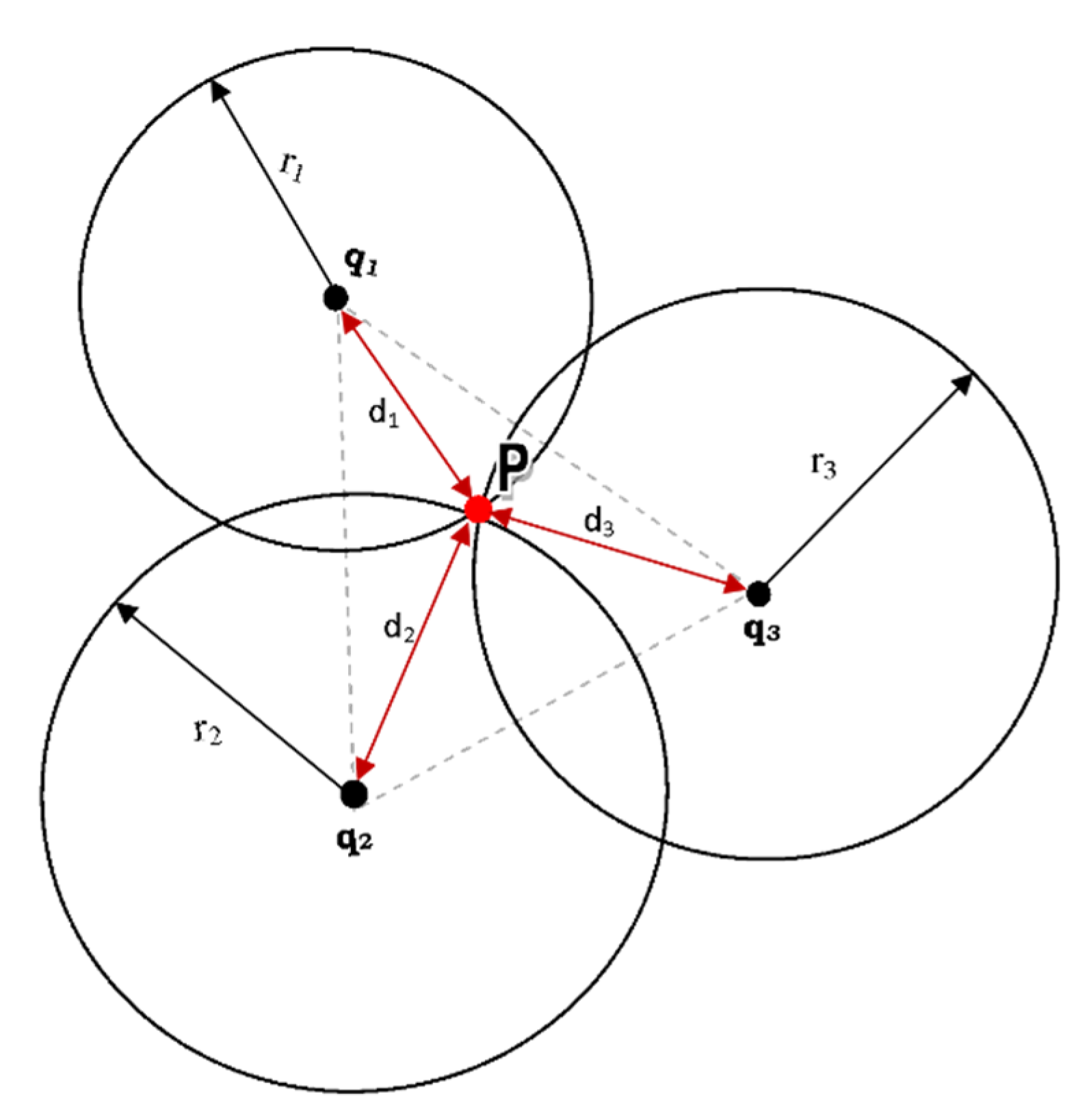
In recent years, a Wireless Sensor Network (WSN) has been widely proposed in several applications where the location information of the sensors has been the fundamental subject of WSN studies [20]. The localization of the exact location can improve the importance of the sensing information. Thus, accurate node localization remains an interesting area of research regarding WSN. Although most localization algorithms offer fairly accurate estimates of the location [21], they have a high computational and communicational complexity.

Based on the distance estimation technique, node localization can be categorized into two categories—range-free localization and range-based localization. The range-free localization method focuses on connectivity information and geometric distance, such as a hop count for node localization [22,23]. However, this method is a well-known cost-effective method that produces poor localization accuracy [22]. On the other hand, the range-based localization method produces approximated results with a higher localization accuracy. This is due to the process of estimating the physical distance between any two sensor nodes [23]. Hence, this research will focus on range-based localization for the best localization accuracy.

For range-based localization, the physical distances between the nodes are first estimated through the physical characteristics of communication signal, which is also called the ranging technique, followed by a localization computation technique to localize the nodes [6,24,25]. Ranging techniques that are used to estimate the distance between the nodes are known as Received Signal Strength Indicator (RSSI), Time of Arrival (ToA), Time Difference of Arrival (TDoA) or Angle of Arrival (AoA) [6]. However, the problem occurs when estimating the distances between two non-neighboring nodes. Hence, the Received Signal Strength Indicator (RSSI) is used to estimate the distances for neighboring nodes while trilateration is introduced to calculate the distances for non-neighboring nodes.

Zhao et al. in [26] proposed an RSSI-based algorithm, which made use of the RSSI values calculated between a sensor node and mobile anchor node for sensor node localization. Moreover, there are some studies that proposed the hybrid implementation of the RSSI-based algorithm, such as the RSSI–ToA-based localization algorithm. Zhang et al. proposed an integrated algorithm which combines the RSSI–ToA-based algorithm with the single mobile anchor node strategy in [27]. Sharma et al., in [22], proposed a RSSI–ToA-based localization algorithm which implements the RSSI technique in the near end and the ToA technique in the far end. Once the ranging values between the anchor node and the unknown node are calculated, node localization is done using the maximum-likelihood (ML) estimation.

However, Heurtefeux and Valois stated that the implementation of the RSSI-based localization algorithm in real environments has low computational accuracy. This is because the signal strength of RSSI is affected by three phenomena, which are path loss (electromagnetic wave power density reduction), fading (weakening signal due to signal deviation) and shadowing (loss of signal due to obstacles) [28]. Hence, this paper will propose the implementation of the RSSI ranging technique for the distance estimation of neighboring nodes and the trilateration technique for the non-neighboring nodes.

2.2. Trilateration

Generally, trilateration is a technique used to estimate the location of an object by measuring the distances from at least three non-collinearly located reference nodes, using the geometry of spheres or triangles [8,9,29]. In practical, trilateration is widely implemented since it is fully distributed, promotes easy implementation and offers low communicational and computational complexity [30]. Distance estimation between two nodes in WSN is possible if they are neighbors, where the distances between the sensors are less than or equal to the communication range. d is the distance between two nodes and r is their communication range; therefore, both sensors are neighbors of each other if $d\le r$.

In this paper, RSSI is used for neighboring nodes while trilateration is used for non-neighboring nodes. Trilateration can recover the positions of the individual sensors based on the Euclidean Distance Matrix (EDM), and at least three or more anchor nodes. Since we are dealing with 2-dimensional WSN, at least three anchor nodes are required for the trilateration process, as shown in Figure 1. Assume that three anchor nodes $q_1,q_2,q_3$ are known, and we want to figure out the coordinate $p$ of an unknown node from only knowing the distances $d_1,d_2,d_3$ and where $d_i=\Vert p-q_i\Vert$ and the distances between the anchor nodes themselves, $d_{i,j}=\Vert q_i-q_j\Vert$ [31]. Hence, it is possible to localize sensor nodes in a network by iterative trilateration [32].

Once the distance estimation process is completed, the information will be transformed into EDM and matrix completion via Nuclear-Norm Minimization (NNM) will take place. Next, NNM will be solved iteratively by using the proposed method, which is the Singular Value Thresholding (SVT) algorithm, which will be discussed in Section 3.

3. The Singular Value Thresholding Algorithm

The basic approach in solving matrix completion is by formulating the rank-minimization problem (RMP). The general matrix RMP is given as

$$\min rank(X)$$

(1)

Subject to

$$A\cdot vec(X)=b$$

where $vec(X)$ denotes a large vector where all the columns are stacked on top of each other. In this paper, the $vec$ notation will be omitted, and is written as $A(X)$ instead of $A\cdot vec(X)$. Hence, the general matrix RMP can now be expressed as

$$\min rank(X)$$

(2)

Subject to

$$A(X)=b$$

where $X$ is the decision variable, rank $(X)$ is the same as the rank of matrix $\mathrm{A},\mathrm{A}\in {\Re }^{mx{n}^2}$ and $b\in {\Re }^m$. This method is acceptable for data fitting, however this algorithm is a nonconvex optimization. Thus, it is NP-hard (non-deterministic polynomial time hard) and too expensive for acquiring exact solutions [10]. By definition, Z is simply the number of singular values available. The sum of the singular values is known as the nuclear norm. Since EDM is a symmetric positive semidefinite matrix, a simple yet effective heuristic is applicable where its trace is minimized instead of its rank. This heuristic is called a nuclear-norm heuristic, or the minimization of the nuclear norm, or singular values of the matrix, as stated by Fazel et al. in [32,33]. This method is known as a convex function, which can be optimized simply via semidefinite programming (SDP) [14]. Hence, nuclear-norm minimization (NNM) is introduced to minimize the nuclear norm of the matrix over the linear equality constraint,

$${\Vert X\Vert }_{\ast }={\displaystyle {\sum }_{i=1}^r{\sigma }_i(X)}$$

(3)

$${\sigma }_i(X)=\sqrt{{\lambda }_i(X^{T}X)}$$

(4)

where ${\sigma }_i(X)$ denotes the singular value of $X$, and ${\Vert X\Vert }_{\ast }$ is known as the nuclear norm, Schatten 1-norm, trace class norm or Ky-fan r-norm [31]. The optimization heuristic is given by:

$$\min {\Vert X\Vert }_{\ast }$$

(5)

Subject to

$$X_{ijk}=a_{ijk},(i,j,k)\in \mathsf{\Omega }$$

For a convex problem, ${\Vert X\Vert }_{\ast }={\Vert \sigma (X)\Vert }_1$, therefore

$$\min {\Vert \sigma (X)\Vert }_1$$

(6)

Subject to

$$X_{ijk}=a_{ijk},(i,j,k)\in \mathsf{\Omega }$$

Now, let $P_{\mathsf{\Omega }}$ be the orthogonal projector onto the span of matrices vanishing outside $\mathsf{\Omega }$ so that the $(i,j)th$ component of $P_{\mathsf{\Omega }}(X)$ is equal to $X_{ij}$ if $(i,j\in \mathsf{\Omega }$, and zero otherwise. The problem can now be expressed as

$$\min {\Vert X\Vert }_{\ast }$$

(7)

Subject to

$$P_{\mathsf{\Omega }}(X)=P_{\mathsf{\Omega }}(M).$$

Nuclear Norm Minimization (NNM) is one of the recent yet effective techniques that have been introduced for node localization. However, as it requires the implementation of SDP, it has another limitation, where the best SDP solvers only work for matrices with sizes of less than 100 × 100 [34].

Therefore, SVT is introduced to solve NNM iteratively to produce a better approximation to the rank of the matrix [14]. SVT is an extension of the method of the iterative soft-thresholding algorithm. This algorithm executes a soft-thresholding operation on a sparse matrix, and the rank of the iterate $X^k$ is empirically nondecreasing, which makes this algorithm well-suited for low-rank matrix completion problems. This algorithm not only ascertains a sparse singular vector but also the basis of the sparse representation.

First, singular value shrinkage operator, $D_{\tau }$ is introduced [20].

Definition 1.

Consider the singular value decomposition of a matrix$X\in {\Re }^{mxn}$of rank r,

$$X=U\sum V^T,\sum =diag(\{{\sigma }_i\}1\le i\le r)$$

(8)

Which defines the singular value shrinkage operator,$D_T$:

$$D_{\tau }(X)=U{D}_{\tau }(\sum )V^T,D^T(\sum )=diag({\{{\sigma }_i-\tau \}}_{+})$$

(9)

The following theorem then follows:

Theorem 1.

For each$\tau \ge 0$and$Y\in {\Re }^{mxn}$, we have

$$D_{\tau }(Y)=\arg \underset{x}{\min }\frac{1}{2}{\Vert X-y\Vert }_F^2+\tau {\Vert X\Vert }_{\ast }$$

(10)

For some fixed$\tau \ge 0$the objective function is set as$f_{\tau }(X)=\frac{1}{2}{\Vert X\Vert }_F^2+\tau {\Vert X\Vert }_{\ast }$, then our optimization problem can be written as

$$\min f_{\tau }(X)$$

(11)

Subject to

$$f_i(X)\le 0,i=1,\dots ,m.$$

where$X$is the decision variable,$f_{\tau }(X)$is the objective function,$\mathrm{A}\in {\Re }^{mx{n}^2}$and$b\in {\Re }^m$.

Let$F(X):=(f_1(X),\dots ,f_m(X))$. Then, the Lagrange function of (11) is

$$L\left(X,y\right)=f_{\tau }(X)+\langle y,F(X)\rangle ,$$

(12)

where$X\in {\Re }^{n_{1}x{n}_2}$, and$y\in {\Re }^m$is a vector with nonnegative components which denoted as$y\ge 0$. This gives

$$\{\begin{array}{c}{X}^k=\arg \min \{f_{\tau }(X)+\langle y^{k-1},F(X)\rangle \},\\ y^k={[y^{k-1}+{\delta }_{k}F(X^k)]}_{+}\end{array}$$

(13)

$x_{+}$is the vector with entries equal to$\max (x_i,0).$When F is an affine mapping of the form$b-A(X),$this can be simplified as

$$\{\begin{array}{c}{X}^k=D_{\tau }(A^{\ast }(y^{k-1})),\\ y^k={[y^{k-1}+{\delta }_k(b-A(X^k))]}_{+}\end{array}$$

(14)

At each step, the computation of SVD is needed and elementary matrix operations will be performed. Equation (10) is the linearized Bregman iteration, which is a special example of Uzawa’s algorithm.

4. Simulation

In this paper, sensor nodes are generated as 2xn matrices while random objects are modelled as circles of similar sizes, according to the given radius, which represent the obstacles between the nodes. The sensor nodes are placed on the plane randomly. If the sensor nodes fall on an object during placement, the sensor will be regenerated. The process is continued by the placement of the sensor nodes on the plane. The dimension of the field is set to be $200\times 200$, as can be seen in Figure 2. Here, we check whether the sensor nodes fall on an object during placement. If this happens, the sensor nodes will be regenerated.

Next, the distances between neighboring nodes are calculated with respect to the x-axis and y-axis. The process of distance estimation is done using the technique of trilateration which make use of Equations (10) and (16). The distances are then transformed into the Euclidean Distance Matrix (EDM), as can be seen in Figure 2. The distance between the non-neighboring nodes can be calculated using the following steps:

• Calculate the distance between coordinate p and anchor node, $d_i=\Vert p-q_i\Vert$. Then, we have

  $${\Vert p-q_i\Vert }^2={\Vert p\Vert }^2-2\langle q_i,p\rangle +{\Vert q_i\Vert }^2=d_i{}^2$$

  (15)
  Subtracting the equations, we get a system of three linear equations with three unknowns (the entries of p);

  $$A=2\left(\begin{array}{c}{(q_2-q_1)}^T\\ {(q_3-q_1)}^T\\ {(q_4-q_1)}^T\end{array}\right),b=\left(\begin{array}{c}{d}_1{}^2-d_2{}^2+{\Vert q_2\Vert }^2-{\Vert q_1\Vert }^2\\ d_1{}^2-d_3{}^2+{\Vert q_3\Vert }^2-{\Vert q_1\Vert }^2\\ d_1{}^2-d_4{}^2+{\Vert q_4\Vert }^2-{\Vert q_1\Vert }^2\end{array}\right)$$

  (16)
• Solve p by solving $A(X)=b$.
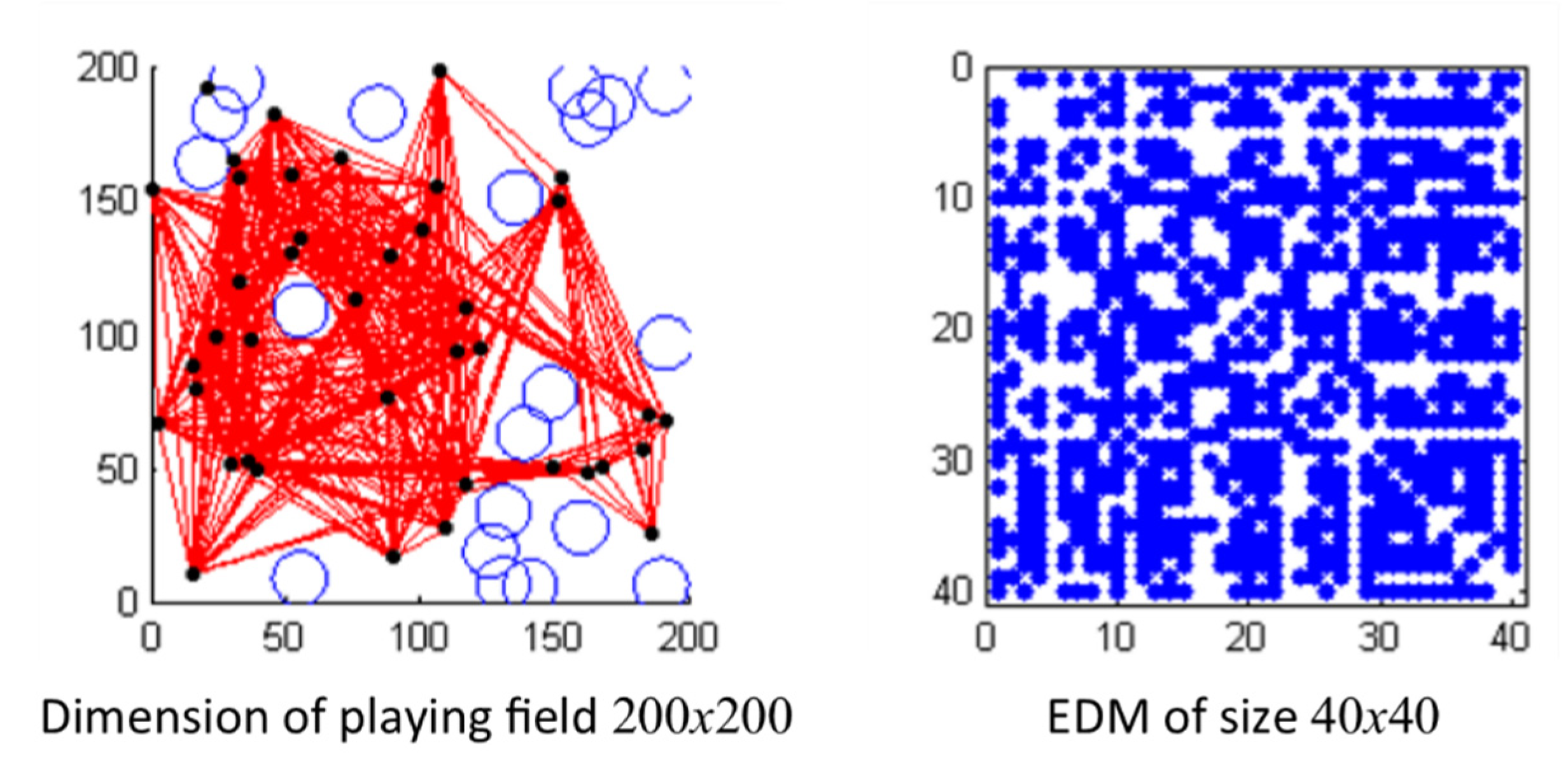
• The results of p are transformed into the Euclidean Distance Matrix (EDM).

In Figure 2, the distances between the neighboring nodes are connected by red lines; whereas, for non-neighboring nodes, their distances are calculated by solving $A(X)=b$ which is done using the method of trilateration. The distances that have been calculated will be transformed into the partial EDM and, hence, will proceed with the process of matrix completion, as explained in Section 4.1.

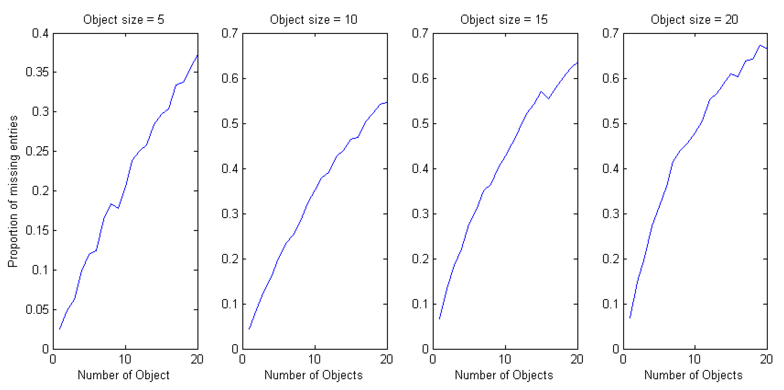
4.1. Matrix Completion

First, the partial EDM is decomposed using SVD. The decomposition produces an array of singular value matrices with respect to the x-axis and y-axis, in which

$$EDM=U\sum V^{\ast }$$

(17)

where $\sum$ is the singular value matrix.

Next, the matrix completion process is continued using Nuclear Norm Minimization (NNM) with the implementation of two techniques—Semidefinite Programming (SDP) and Singular Value Thresholding (SVT).

4.2. Nuclear Norm Minimization (NNM)

This technique optimizes array of singular value matrices subject to limited known constraints by using two algorithms, which are Semidefinite Programming (SDP) and Singular Value Thresholding (SVT).

4.2.1. Semidefinite Programming (SDP)

Let $C(X)$ be the linear function of $X$ and $b$ is the singular value matrix. Then

$$SDP:\min C•X$$

Subject to

$$\begin{array}{l}{A}_i•X=b_i,i=1,\dots ,m,\\ X_{ij}=a_{ij},\left(i,j\right)\in \mathsf{\Omega },\\ X\ge 0\end{array}$$

(18)

This is done by using the CVX toolbox in MATLAB [35].

4.2.2. Singular Value Thresholding

$$\min f_{\tau }(X)$$

(19)

Subject to

$$f_i(X)\le 0,i=1,\dots ,m.$$

where $X$ is the decision variable, $f_{\tau }(X)$ is the objective function, $\mathrm{A}\in {\Re }^{mx{n}^2}$ and $b\in {\Re }^m$.

With

$$\{\begin{array}{c}{X}^k=D_{\tau }(A^{\ast }(y^{k-1})),\\ y^k={[y^{k-1}+{\delta }_k(b-A(X^k))]}_{+}\end{array}$$

(20)

The optimization is done by using two techniques which are Convex Optimization through Semidefinite Programming (SDP) and also via Singular Value Thresholding (SVT). The optimization is done using MATLAB. Once the optimization process is completed, the location of the sensors can be located.

5. Results and Discussions

The average number of missing entries in the EDM is computed for a range of 1 to 20 sensors. The average is calculated by generating 100 random scenarios for each number of obstacles.

Figure 3 shows the relationship between the number and size of objects and its effect on the proportion of missing entries. The proportion of missing entries increased as the number and size of the objects increased. This shows that a greater number of objects (obstacles), or the larger size of the objects, will both inevitably result in a greater number of missing entries in the Euclidean Distance Matrix (EDM).

Based on this result, the number and size of objects in this paper are fixed to five objects with a size of 8 cm.

• Next, matrix completion is implemented using Singular Value Thresholding in MATLAB and the results are attached in Appendix 1.
• The complete EDM is now reconstructed via the technique of Trilateration in MATLAB and the results are stated in

  Table 1. Experimental results for 2-dimensional Wireless Sensor Network localization via Semidefinite Programming (CVX Toolbox).

  Nu. of Sensor Node	Percentage of Missing Entries (%)	Relative Error on EDM	Relative Recovery Error	Processing Time (s)
  10	20	4.89 × 10−5	4.31 × 10−1	0.04872
  20	25	6.21 × 10−4	5.23 × 10−1	0.08231
  50	40	6.89 × 10−4	5.65 × 10−1	1.14435
  100	60	5.23 × 104	3.57 × 105	2.23154
  200	80	4.23 × 104	5.38 × 107	6.5134

  .

Our computational results are displayed in Table 1 and

Table 2. Experimental results for 2-dimensional Wireless Sensor Network localization via Singular Value Thresholding.

Nu. of Sensor Node	Nu. of Iteration	Percentage of Missing Entries (%)	Relative Error on EDM	Relative Recovery Error	Processing Time (s)
10	17	26	5.64 × 10−5	6.26 × 10−1	0.036282
20	11	24	5.27 × 10−5	6.51 × 10−1	0.039764
50	9	22.4	3.82 × 10−5	6.24 × 10−1	0.081020
100	7	18.1	4.85 × 10−5	5.59 × 10−1	0.637559
200	7	19.1	5.77 × 10−5	5.27 × 10−1	2.720775

. Table 1 states the number of sensor nodes deployed, percentage of missing entries, percentage of missing entries in the incomplete EDM, the relative error of EDM, relative recovery error and the run time in seconds for 2-dimensional Wireless Sensor Network localization via Semidefinite Programming (CVX Toolbox). Table 2 states the number of sensor nodes deployed, number of iterations needed for convergence, percentage of missing entries in the incomplete EDM, the run time in seconds, the relative error of EDM and relative recovery error for 2-dimensional Wireless Sensor Network localization via Singular Value Thresholding.

Table 1 shows that, for a number of sensor nodes less than 100, WSN localization via SDP by using CVX toolbox works quite well, with 4.529 × 10⁻⁴ and 5.06 × 10¹ as the average relative error of EDM and the average relative recovery error, respectively. However, as stated in [35], where the best SDP solvers only work for matrices with sizes of less than 100 × 100, it can be seen that the relative error of EDM and relative recovery error of the reconstructed node location are high for sensor nodes with 100 or more nodes. Therefore, although the SDP method is simple and user-friendly with the application of CVX toolbox in MATLAB, the method is proven to have limitations in the number of sensor nodes, which affects the size of the EDM.

On the contrary, we can see in Table 2 that the proposed technique produces a stable relative error of EDM and relative recovery error of the reconstructed node location for all sensor nodes. The number of missing nodes depends on the percentage of missing entries that are produced during the simulation. Since the number and size of objects in this simulation are fixed to five objects with sizes of 8 cm, as the number of sensor nodes increases, the number of missing entries will be decreasing. The average relative recovery error of the reconstructed node location via SVT is 5.974 × 10⁻¹, while the average relative error for matrix completion via SVT is 5.074 × 10⁻⁵.

6. Conclusions

This research proposes the implementation of Singular Value Thresholding along with the application of Nuclear Norm Minimization (NNM) for 2-dimensional (2-D) Wireless Sensor Network localization (with obstacles). The process of matrix completion via SVT produces a low average relative error, which is 5.074 × 10⁻⁵. However, the average relative recovery error of the reconstructed node location is 5.974 × 10⁻¹ which can be improvised, referring to the lower matrix completion’s relative error. Further work is needed to improvise the process of node reconstruction.

References

1. Verdone, R.; Dardari, D.; Mazzini, G.; Conti, A. Wireless Sensor and Actuator Networks: Technologies, Analysis and Design; Academic Press: London, UK, 2010. [Google Scholar]
2. Jiang, J.-A.; Zheng, X.-Y.; Chen, Y.-F.; Wang, C.-H.; Chen, P.-T.; Chuang, C.-L.; Chen, C.-P. A Distributed RSS-Based Localization Using a Dynamic Circle Expanding Mechanism. IEEE Sens. J. 2013, 13, 3754–3766. [Google Scholar] [CrossRef]
3. Tomasi, C.; Kanade, T. Shape and motion from image streams: A factorization method. Proc. Natl. Acad. Sci. USA 2013, 90, 9795–9802. [Google Scholar] [CrossRef] [Green Version]
4. Abernethy, J.; Bach, F.; Evgeniou, T.; Vert, J.-P. Low-rank matrix factorization with attributes. arXiv 2006, arXiv:cs/0611124, 1–12. [Google Scholar]
5. Mesbahi, M.; Papavassilopoulos, G.P. On the Rank Minimization Problem over a Positive Semidefinite Linear Matrix Inequality. IEEE Trans. Autom. Control 1997, 42, 239–243. [Google Scholar] [CrossRef]
6. Chaurasiya, V.K.; Jain, N.; Nandi, G. A novel distance estimation approach for 3D localization in wireless sensor network using multi dimensional scaling. Inf. Fusion 2014, 15, 5–18. [Google Scholar] [CrossRef]
7. Brida, P.; Machaj, J. A Novel Enhanced Positioning Trilateration Algorithm Implemented for Medical Implant In-Body Localization. Int. J. Antennas Propag. 2013, 2013, 1–10. [Google Scholar] [CrossRef]
8. Thomas, F.; Ros, L. Revisiting trilateration for robot localization. IEEE Trans. Robot. 2005, 21, 93–101. [Google Scholar] [CrossRef] [Green Version]
9. Patil, S.; Zaveri, M. MDS and Trilateration Based Localization in Wireless Sensor Network. Wirel. Sens. Netw. 2011, 3, 198–208. [Google Scholar] [CrossRef] [Green Version]
10. Smith, R.S. Frequency Domain Subspace Identification Using Nuclear Norm Minimization and Hankel Matrix Realizations. IEEE Trans. Autom. Control 2014, 59, 2886–2896. [Google Scholar] [CrossRef] [Green Version]
11. Zhang, L.; Yang, T.; Jin, R. Analysis of Nuclear Norm Regularization for Full-rank Matrix Completion. arXiv 2009, arXiv:1504.06817 [cs.LG]. Available online: https://arxiv.org/abs/1504.06817v1 (accessed on 20 November 2019).
12. Blomberg, N.; Rojas, C.R.; Wahlberg, B. Approximate Regularization Paths for Nuclear Norm Minimization Using Singular Value Bounds—With Implementation and Extended Appendix. arXiv 2015, arXiv:1504.05208 [cs.SY]. Available online: https://arxiv.org/abs/1504.05208v1 (accessed on 25 November 2019).
13. Mardani, M.; Mateos, G.; Giannakis, G.B. Distributed nuclear norm minimization for matrix completion. In Proceedings of the 2012 IEEE 13th International Workshop on Signal Processing Advances in Wireless Communications (SPAWC), Cesme, Turkey, 17–20 June 2012; pp. 354–358. [Google Scholar] [CrossRef]
14. Cai, J.-F.; Candés, E.J.; Shen, Z. A Singular Value Thresholding Algorithm for Matrix Completion. SIAM J. Optim. 2010, 20, 1956–1982. [Google Scholar] [CrossRef]
15. Oh, T.H.; Matsushita, Y.; Tai, Y.W.; Kweon, I.S. Fast randomized singular value thresholding for low-rank optimization. IEEE Trans. Pattern Anal. Mach. Intell. 2017, 40, 376–391. [Google Scholar] [CrossRef] [PubMed] [Green Version]
16. Nguyen, L.T.; Kim, J.; Kim, S.; Shim, B. Localization of iot networks via low-rank matrix completion. IEEE Trans. Commun. 2019, 67, 5833–5847. [Google Scholar] [CrossRef]
17. Feng, C.; Valaee, S.; Sy, W.; Au, A.; Tan, Z. Localization of Wireless Sensors via Nuclear Norm for Rank Minimization. In Proceedings of the 2010 IEEE Global Telecommunications Conference GLOBECOM 2010, Miami, FL, USA, 6–10 December 2010; pp. 1–5. [Google Scholar] [CrossRef]
18. Candes, E.J.; Recht, B. Exact Matrix Completion via Convex Optimization. Found. Comp. Math 2009, 9, 1–49. [Google Scholar] [CrossRef] [Green Version]
19. Varga, A.K. Localization Techniques in Wireless Sensor Networks. Prod. Syst. Inf. Eng. 2013, 6, 81–90. [Google Scholar]
20. Liu, B.-C.; Lin, K.-H. Accuracy Improvement of SSSD Circular Positioning in Cellular Networks. IEEE Trans. Veh. Technol. 2011, 60, 1766–1774. [Google Scholar] [CrossRef]
21. Eren, T.; Goldenberg, O.K.; Whiteley, W.; Yang, Y.R.; Morse, A.S.; Anderson, B.D.O.; Belhumeur, P.N. Rigidity, computation, and randomization in network localization. In Proceedings of the IEEE INFOCOM, Hong Kong, China, 7–11 March 2014; Volume 4, pp. 2673–2684. [Google Scholar] [CrossRef]
22. Sharma, G.; Kumar, A. Improved range-free localization for three-dimensional wireless sensor networks using genetic algorithm. Comput. Electr. Eng. 2018, 72, 808–827. [Google Scholar] [CrossRef]
23. Zhou, C.; Yang, Y.; Wang, Y. DV-Hop localization algorithm based on bacterial foraging optimization for wireless multimedia sensor networks. Multimed. Tools Appl. 2019, 78, 4299–4309. [Google Scholar] [CrossRef]
24. Yan, X.; Luo, Q.; Yang, Y.; Liu, S.; Li, H.; Hu, C. ITL-MEPOSA: Improved Trilateration Localization with Minimum Uncertainty Propagation and Optimized Selection of Anchor Nodes for Wireless Sensor Networks. IEEE Access 2019, 7, 53136–53146. [Google Scholar] [CrossRef]
25. Manickam, M.; Selvaraj, S. Range-based localisation of a wireless sensor network using Jaya algorithm. IET Sci. Meas. Technol. 2019, 13, 937–943. [Google Scholar] [CrossRef]
26. Zhao, Y.; Xu, J.; Jiang, J. RSSI based localization with mobile anchor for wireless sensor networks. In Proceedings of the 2017 International Conference on Geo-Spatial Knowledge and Intelligence, Chiang Mai, Thailand, 8–10 December 2018; pp. 176–187. [Google Scholar] [CrossRef] [Green Version]
27. Zhang, L.; Yang, Z.; Zhang, S.; Yang, H. Three-Dimensional Localization Algorithm of WSN Nodes Based on RSSI-TOA and Single Mobile Anchor Node. J. Electr. Comput. Eng. 2019. [Google Scholar] [CrossRef] [Green Version]
28. Heurtefeux, K.; Valois, F. Is RSSI a Good Choice for Localization in Wireless Sensor Network? In Proceedings of the 2012 IEEE 26th International Conference on Advanced Information Networking and Applications, Fukuoka, Japan, 26–29 March 2012; pp. 732–739. [Google Scholar] [CrossRef]
29. Yang, Z.; Liu, Y.; Li, X.-Y. Beyond Trilateration: On the Localizability of Wireless Ad Hoc Networks. IEEE/ACM Trans. Netw. 2010, 18, 1806–1814. [Google Scholar] [CrossRef]
30. Fazel, M. Matrix Rank Minimization with Applications. Ph.D. Thesis, Stanford University, Stanford, CA, USA, 2002. [Google Scholar]
31. Mao, G.; Fidan, B.; Anderson, B.D. Wireless sensor network localization techniques. Comput. Netw. 2007, 51, 2529–2553. [Google Scholar] [CrossRef]
32. Fazel, M.; Hindi, H.; Boyd, S. A rank minimization heuristic with application to minimum order system approximation. In Proceedings of the 2001 American Control Conference. (Cat. No.01CH37148), Arlington, VA, USA, 25–27 June 2001; Volume 6, pp. 4734–4739. [Google Scholar] [CrossRef] [Green Version]
33. Recht, B.; Xu, W.; Hassibi, B. Necessary and sufficient conditions for success of the nuclear norm heuristic for rank minimization. In Proceedings of the 2008 47th IEEE Conference on Decision and Control, Cancun, Mexico, 9–11 December 2008; pp. 3065–3070. [Google Scholar] [CrossRef]
34. Najib, Y.N.A. Matrix Completion. Master’s Thesis, University of Manchester, Manchester, UK, 2013. [Google Scholar]
35. Michael, G.; Stephen, B. CVX: Matlab Software for Disciplined Convex Programming; Version 2.0 Beta. Available online: http://cvxr.com/cvx (accessed on 20 November 2019).
Figure 1. Intersection of three anchor nodes and new coordinate p .
Mathematics 08 00437 g001
Figure 2. Sensors and the partial Euclidean Distance Matrix (EDM). Left: black dots represent the sensors, blue circles represent the objects, while red lines connect the neighboring sensors (nodes). Right: blue dots represent the entries in the Euclidean Distance Matrix, corresponding to the neighboring sensors (nodes).
Mathematics 08 00437 g002
Figure 3. Graphs of the effects of object size to the proportion of missing entries for object size equal to 5, 10, 15, and 20 cm.
Mathematics 08 00437 g003