Abstract
In this paper, we consider evolutionary games and construct a model of replicator dynamics with bounded continuously distributed time delay. In many circumstances, players interact simultaneously while impacts of their choices take place after some time, which implies a time delay exists. We consider the time delay as bounded continuously distributed other than some given constant. Then, we investigate the stability of the evolutionarily stable strategy in the replicator dynamics with bounded continuously distributed time delay in two-player game contexts. Some stability conditions of the unique interior Nash equilibrium are obtained. Finally, the simple but important Hawk–Dove game is used to verify our results.
1. Introduction
Traditional game theory considers agents are always completely rational or sometimes even super-rational (see Aumann [1]). Evolutionary game theory provides a fundamental theoretical framework for analyzing interactions in a large population of agents who are myopic and adjust their choices in the context of continuous interactions. Maynard Smith [2] proposed the fundamental notion of an evolutionarily stable strategy (ESS), which captures the robustness of Nash equilibria to the invasion by a small fraction of agents with different behavior. Subsequently, much research around ESS has emerged (see Haigh [3], Vickers [4], Hines [5], Iqbal [6], and Tomkins [7], among others).
Nevertheless, the ESS, being a refinement of Nash equilibria, does not involve the long-run state of the population given an initial configuration. In 1978, Taylor et al. [8] studied the population evolution by a dynamic approach. Their so-called replicator dynamics describes the evolution of frequencies of strategies in as agents compare their payoffs to the total average payoff of the population. Since then, a rich literature of evolutionary game dynamics has been appeared (e.g., Friedman [9], Hofbauer and Sigmund [10], and Hofbauer and Weibull [11]). Hwang and Newton [12] considered populations of agents whose behavior is governed by perturbed best or better response dynamics with perturbation probabilities that depend log-linearly on payoffs. Mertikopoulos and Sandholm [13] studied a class of evolutionary game dynamics defined by balancing a gain determined by the game’s payoffs against a cost of motion that captures the difficulty with which the population moves between states. Thorough, systematic, and high-quality monographs were published by Weibull [14], Sandholm [15], and Tanimoto [16]. It is worth mentioning that Newton [17] provided an excellent review of evolutionary game theory. He surveyed recent progress on evolutionary games for current and potential researchers in this field and discussed open problems and challenges of significance.
On the other hand, based on one population with symmetric, two-player structure, Tanimoto and Sagara [18] defined dilemma games using static and dynamic factors and discussed the impacts of these two factors on the dilemma. Based on the work of Tanimoto [18] and Taylor and Nowak [19], Wang et al. [20] reviewed the universal scaling for the dilemma strength in evolutionary games and proposed new universal scaling parameters for the dilemma strength. Utilizing their new parameters, they perfectly resolved the paradox of cooperation benefits by Németh and Takács [21]. Recently, Hammoud et al. [22] published a marvellous application of evolutionary games. They presented two new models to form cloud federations using genetic algorithm and evolutionary game theory and studied the problem of forming highly profitable federated clouds. Bogomolnaia and Jackson [23] and Diamantoudi and Xue [24] investigated how rational individuals partition themselves into different coalitions in so-called hedonic games where individuals’ preferences depend solely on the composition of the coalition they belong to. They studied conditions of the stability of coalition partition and solutions. A fantastic application considering trust-based hedonic coalitional game can be found in [25]. Wahab et al. [25] proposed a comprehensive trust framework that allows services to establish credible trust relationships in the presence of collusion attacks in which attackers collude to mislead the trust results.
Classic evolutionary dynamics requires individuals to instantaneously react to the system as soon as they observe the outcomes, which means without taking into account the delay effect. This is clearly impossible and unreasonable. Many examples in biology, social sciences, and especially economics reveal that the influence of actions is not immediate and the effects take some time to emerge. For instance, resource regeneration, maturation, growth periods, feeding times, etc. should be taken into account in biological models. Accordingly, it is more realistic to consider impacts of the time delay on evolutionary game models. Tao and Wang [26] investigated effects of a fixed symmetric time delay on the stability of replicator dynamics where the payoffs of strategies at time t rely on the frequency of strategies at time and showed that the stability of evolutionary stable strategy will be lost when the time delay is sufficiently large. Alboszta [27] studied two delay models of discrete replicator dynamics. In their social-type model, large delays result in the instability and stability sustains for any delay in the biological-type. In [28], the authors introduced a population consists of communities. They defined three kind of evolutionary stable strategies and discussed the stability of these ESSs under replicator dynamics with two types of delays. Burridge et al. [29] considered a population of agents playing the Hawk–Dove game with a finite memory of past interactions. They showed an instability occurs at a critical memory length. Long memory is considered to be beneficial but is proved to be unstable.
Related studies show clearly that the time delay can change the dynamic properties of the evolutionary game models. The effects of the time delay may also be an important factor for us to understand the evolution of behavior. However, the literature mentioned above usually assumes that the time delay is fixed, but this assumption is more or less restrictive in reality. For example, returns of economic investments are realized in the future and the time lag is usually uncertain. In addition, in the world of living creatures, it is unrealistic to assume the offspring become mature at the same time. For instance, corn seeds are usually sowed in April and become mature during August to October. Therefore, time delay should not be ignored. Furthermore, concerning different soils, humidity, sunshine, etc., it is impossible to suppose all corn matures simultaneously, which means the time delay should vary. More precisely, the time delay should be continuously distributed other than one or some fixed time delays. Ben-Khalifa et al. [30] considered discrete and continuously distributed delays in replicator dynamics. They investigated the stability of replicator dynamics with different distributed time delay, such as exponential delay distribution, Erlang distribution, and uniform distribution. However, for mathematical convenience, all models studied by Ben [30] use the infinite integral, which means every moment in the past is considered, even the ’infinite history’. In our opinion, this consideration is a bit unrealistic for human and animals since most of them pay no attention to infinite past. Concerning the maturing time of corn, immature corn may have already rotted after a usual maximum ripening time and it makes no sense to assume an infinite growth cycle. Therefore, the assumption of bounded continuously distributed time delay is more reasonable in reality.
The remainder of the paper is organized as follows. In Section 2, we construct our models of replicator dynamics with bounded continuously distributed time delay in the context of game and discuss the stability and instability of the ESS under our models. A simple numerical example of Hawk–Dove game is shown in Section 3 to verify our results and we conclude the paper in Section 4.
2. Replicator Dynamics with Bounded Continuously Distributed Delays
2.1. The Mathematical Model
We consider a large population of individuals who interact repeatedly through random match and assume that our population is haploid as usual. In every competition, there are two options for each player, denoted by and . The outcome is given by the following matrix
and we assume that and .
At time t, denote as the share of strategy and as the fitness or payoff of , . Thus, we have
Let , and . It is well-known from Weibul [14] that there exists a unique mixed ESS, .
In the Introduction, we explain our intuition to consider a bounded continuously distributed time delay. Now, we give the formal definition of such time delay.
Definition 1.
Let τ be a time delay parameter and . τ is a bounded continuously distributed time delay if it randomly distributes on some bounded interval.
Let , , be the number of individuals choosing strategy at time t. Thus, denotes the total number of agents. During a small time interval , we assume fraction of the population takes part in the competition. Simultaneously, we assume is relevant to the corresponding fitness or payoff at every previous time bounded by some maximum delay , which means we deal with bounded continuously distributed time delay. Hence, we derive the following bounded continuously distributed time delay equations
where .
Remark 1.
If the interval to which a bounded continuously distributed time delay belongs reduces to a number, Equation (1) becomes the traditional time delay equation with fixed delay. Thus, our model includes the classic model studied before.
The item in Equation (1) is used to describe the significance of the delay information. Since is nondecreasing about s, we see that the older the information is, the less useful it is. Actually, it can be regarded as a weighting factor.
Then, the total number of agents at time can be written as
where .
From Equation (3), we have:
Furthermore, the corresponding replicator dynamics reads
2.2. Stability Analysis-Special Case
From the theory of delay differential equations, we conclude that the mixed ESS is asymptotically stable if and only if the zeros of characteristic equation of Equation (6) have negative real parts. The next lemma is from Hale [31].
Lemma 1.
For simplicity, we first consider a special simple case of Equation (6) and we omit the kernel function . Then, the linear dynamics in Equation (6) becomes
When , . Thus, Equation (8) is equivalent to
Theorem 1.
The mixed ESS is asymptotically stable if and only if .
Proof.
Suppose that ; we prove all roots of the characteristic in Equation (8) have negative real parts.
If there exists a root of Equation (8) with , , , and . Moreover, we assume that since from complex analysis if is a solution of Equation (8), so is . Substituting into Equation (8) and separating the real and imaginary parts, we have
Furthermore, by a simple variable change, we get
Let , where and ; we have
The first inequality holds since increases on and the following equality due to the periodicity of sine function. Therefore, we have .
Since , we get which implies and .
We next discuss the sign of . If , then since , and , which contradicts with our hypothesis . On the other hand, assume that ; then, we have
Accordingly, we obtain which is a contradiction. This completes the proof of the sufficient condition.
To verify the necessary condition, we only need prove if , then the zero of Equation (9) is unstable. Let and with . We can easily verify that is a root of characteristic of Equation (9), which means the stability is lost. We next show the stability can never be regained.
By differentiating the characteristic in Equation (9) with respect to , we have
2.3. Stability Analysis-General Case
In this subsection, we consider a more realistic situation. We assume that the importance of the different delay information is not uniform and consider weighting factor . Unlike Ben [28], it is more reasonable to consider a given time window, which means bounded continuously distributed delays other than infinite distributed delays. We now testify the stability of the zero solution of the model in Equation (6)
The characteristic equation of the linear system in Equation (10) takes the form of
If we make the assumption of small time delay, Equation (11) can be simplified to a second-order equation by substituting the exponential term with its Taylor expansion and keeping only the linear term. Therefore, we have the following second-order equation
Theorem 2.
The mixed ESS is asymptotically stable for sufficiently small time delay τ.
Proof.
From Lemma 1, the interior Nash equilibrium is asymptotically stable if all the roots of the characteristic equation have negative real parts. Since the equation now is a second-order equation (Equation (12)), the roots have negative real parts if their sum is negative and their product is positive. We notice that and since our assumption that and holds. □
For general case of the time delay, we have
Theorem 3.
The mixed ESS is asymptotically stable if .
Proof.
By separating the real and imaginary parts, we obtain
If , then
Furthermore, we have
where and the last equality holds due to the mean value theorem for integrals.
and this is a contradiction. Then, any characteristic root has negative real part and the mixed ESS is therefore asymptotically stable if . □
Remark 2.
In Theorem 1, we obtain a sufficient and necessary condition for the ESS to be asymptotically stable, while in Theorems 2 and 3 only sufficient conditions are given.
3. Numerical Example
The Hawk–Dove model has been successfully applied to explore animal behavior and its evolution. Many applications exist outside of biology. As we know, the Hawk–Dove game can be regarded as a typical anti-coordination game, all of which have three Nash equilibria, two of which consist of pure strategies and a third of mixed strategies. In the Hawk–Dove game, two individuals compete for a resource. They share a common strategy set with two strategies, Hawk (H) and Dove (D). The strategy H stands for a radical option for the resource while the strategy D represents a gentle behavior of never fighting. The payoff matrix is given as follows
where and . V stands for the value of the resource and C for the cost of fighting against the hawk strategy. The cost is usually high if a fight happens, thus we assume that .
Remark 3.
Excellent applications of game theory using a Stackelberg game approach were presented by Wahab et al. [32,33]. They investigated [32] the problem of community-based cooperation among intelligent Web service agents by modeling the community formation problem as a Stackelberg game model. In 2019, Wahab et al. proposed a comprehensive framework for MTD deployment in the cloud. Their framework comprises several techniques and methods, including a risk assessment methodology and a machine learning approach to collect information from malicious activities. As time delay exists in the process of detection and defense, it is an interesting work in the future to consider the effects of the time delay based on models constructed by Wahab et al.
3.1. Special Case
Our special case is a model without an exponential term, which precisely satisfies
The ESS is asymptotically stable if and only if the time delay is smaller than , as stated in Theorem 1. In the context of hawk and dove games, the delay bound is given as . We depict in Figure 1 the trajectory of numerical solution of the above equation with and . We observe the convergence to the ESS and as the time delay approaches the critical value, the solution oscillatorily converges to the ESS. In Figure 2, as the delay is increased to 3, the system oscillates periodically.
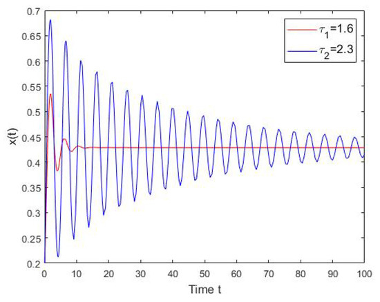
Figure 1.
The numerical solution the system in Equation (14), where and .
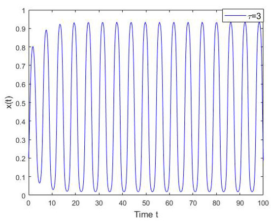
Figure 2.
The oscillation of the solution of system in Equation (14), where = 3.
3.2. General Case
When the exponential term is considered as the kernel function, our model becomes
We prove that the ESS is asymptotically stable for sufficiently small in Theorem 2. In fact, we show in Theorem 3 that the ESS stays stable if . These sufficient conditions are justified in the following figures. Now, the parameters V and C are the same as in the last section. We obtain from the results in Figure 3 that the ESS is asymptotically stable for a small . Setting , from Theorem 3, we know that the ESS is asymptotically stable. This is verified in Figure 4. As remarked in Section 2.2, Theorem 3 is a sufficient condition for stability and it may be too conservative.
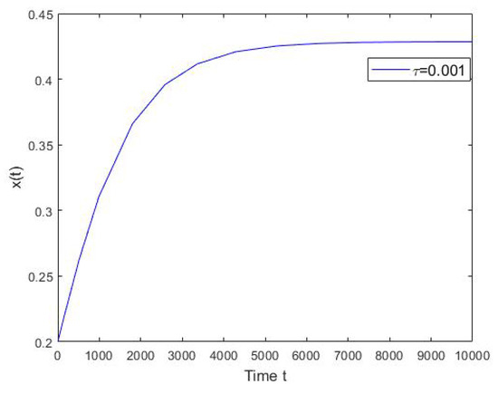
Figure 3.
The numerical solution the system in Equation (15), where and .
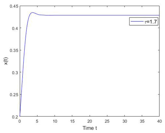
Figure 4.
The numerical solution the system in Equation (15), where and .
4. Conclusions
In this paper, for a class of symmetric games with two strategies, we derive stability conditions of the unique ESS under replicator dynamics with bounded continuously distributed time delay, i.e., a time window for the delay. As remaining topics, it is interesting and meaningful to extend the model to more general settings such as games with more than two strategies or the non-linear payoffs.
Author Contributions
Writing Original Draft Preparation and Project management, C.Z.; Methodology and Formal Analysis, C.Z. and J.W.; Supervision and Writing Review, H.Y. and Z.L. All authors have read and agreed to the published version of the manuscript.
Funding
This research was funded by NSFC (Grant No. 11271098, 61472093), Guizhou Province University Science and Technology Top Talents Project (Grant No. KY[2018]047), Guizhou University of Finance and Economics (Grant No. 2018XZD01).
Conflicts of Interest
The authors declare no conflict of interest.
References
- Aumann, R.J. Rationality and bounded rationality. Games Econ. Behav. 1997, 21, 2–14. [Google Scholar] [CrossRef]
- Maynard Smith, J. The theory of games and the evolution of animal conflicts. J. Theor. Biol. 1974, 47, 209–221. [Google Scholar] [CrossRef]
- Haigh, J. Game theory and evolution. Adv. Appl. Probab. 1975, 7, 8–11. [Google Scholar] [CrossRef]
- Vickers, G.T.; Cannings, C. On the definition of an evolutionarily stable strategy. J. Theor. Biol. 1987, 129, 349–353. [Google Scholar] [CrossRef]
- Hines, W.G.S. Evolutionary stable strategies: A review of basic theory. Theor. Popul. Biol. 1987, 31, 195–272. [Google Scholar] [CrossRef]
- Iqbal, A.; Toor, A.H. Evolutionarily stable strategies in quantum games. Phys. Lett. A. 2001, 280, 249–256. [Google Scholar] [CrossRef]
- Tomkins, J.L.; Hazel, W. The status of the conditional evolutionarily stable strategy. Trends. Ecol. Evol. 2007, 22, 522–528. [Google Scholar] [CrossRef]
- Taylor, P.D.; Jonker, L.B. Evolutionary stable strategies and game dynamics. Math. Biosci. 1978, 40, 145–156. [Google Scholar] [CrossRef]
- Friedman, D. Evolutionary games in economics. Econometrica 1991, 59, 637–666. [Google Scholar] [CrossRef]
- Hofbauer, J.; Weibull, J.W. Evolutionary selection against dominated strategies. J. Econ. Theory 1996, 71, 558–5739. [Google Scholar] [CrossRef]
- Hofbauer, J.; Sigmund, K. Evolutionary game dynamics. Bull. Am. Math. Soc. 2003, 40, 479–519. [Google Scholar] [CrossRef]
- Hwang, S.; Newton, J. Payoff-dependent dynamics and coordination games. Econ Theory 2017, 64, 589–604. [Google Scholar] [CrossRef]
- Mertikopoulos, P.; Sandholm, W.H. Riemannian game dynamics. J. Econ. Theory 2018, 177, 315–364. [Google Scholar] [CrossRef]
- Weibull, J. Evolutionary Game Theory; MIT Press: Cambridge, MA, USA, 1995. [Google Scholar]
- Sandholm, W.H. Population Games and Evolutionary Dynamics; Economic Learning and Social Evolution; MIT Press: Cambridge, MA, USA, 2010. [Google Scholar]
- Tanimoto, J. Fundamentals of Evolutionary Game Theory and its Applications; Springer: Tokyo, Japan, 2015. [Google Scholar]
- Newton, J. Evolutionary Game Theory: A Renaissance. Games 2018, 9, 31. [Google Scholar] [CrossRef]
- Tanimoto, J.; Sagara, H. Relationship between dilemma occurrence and the existence of a weakly dominant strategy in a two-player symmetric game. Biosystems 2007, 90, 105–114. [Google Scholar] [CrossRef] [PubMed]
- Taylor, C.; Nowak, M. Transforming the Dilemma. Evolution 2007, 61, 2281–2292. [Google Scholar] [CrossRef]
- Wang, Z.; Kokubo, S.; Jusup, M.; Tanimoto, J. Universal scaling for the dilemma strength in evolutionary games. Phys. Life. Rev. 2015, 14, 1–30. [Google Scholar] [CrossRef]
- Németh, A.; Takács, K. The paradox of cooperation benefits. J. Theor. Biol. 2010, 264, 301–311. [Google Scholar] [CrossRef]
- Hammoud, A.; Mourad, A.; Otrok, H.; Wahab, O.A.; Harmanani, H. Cloud federation formation using genetic and evolutionary game theoretical models. Future Gener. Comp. Syst. 2020, 104, 92–104. [Google Scholar] [CrossRef]
- Bogomolnaia, A.; Jackson, M.O. The stability of hedonic coalition structures. Games Econ. Behav. 2002, 38, 201–230. [Google Scholar] [CrossRef]
- Diamantoudi, E.; Xue, L. Farsighted stability in hedonic games. Soc Choice Welf. 2003, 21, 39–61. [Google Scholar] [CrossRef]
- Wahab, O.A.; Bentahar, J.; Otrok, H.; Mourad, A. Towards trustworthy multi-cloud services communities: A trust-based hedonic coalitional game. IEEE Trans. Serv. Comput. 2018, 11, 184–210. [Google Scholar] [CrossRef]
- Tao, Y.; Wang, Z. Effect of time delay and evolutionarily stable strategy. J. Theor. Biol. 1997, 187, 111–116. [Google Scholar] [CrossRef]
- Alboszta, J.; Miȩkisz, Z. Stability of evolutionarily stable strategies in discrete replicator dynamics with time delay. J. Theor. Biol. 2004, 187, 175–179. [Google Scholar]
- Ben Khalifa, N.; El-Azouzi, R.; Hayel, Y.; Mabrouki, I. Evolutionary games in interacting communities. Dyn. Games Appl. 2017, 7, 131–156. [Google Scholar] [CrossRef]
- Burridge, J.; Gao, Y.; Mao, Y. Delayed response in the Hawk Dove game. Eur. Phys. J. B 2017, 90, 13. [Google Scholar] [CrossRef]
- Ben Khalifa, N.; El-Azouzi, R.; Hayel, Y. Discrete and continuous distributed delays in replicator dynamics. Dyn. Games Appl. 2018, 8, 713–732. [Google Scholar] [CrossRef]
- Hale, J.K.; Verduyn Lunel, S.M. Introduction to Functional Differential Equations; Applied Mathematical Sciences; Springer: New York, NY, USA, 1993. [Google Scholar]
- Wahab, O.A.; Bentahar, J.; Otrok, H.; Mourad, A. A Stackelberg game for distributed formation of business-driven services communities. Expert Syst. Appl. 2016, 45, 359–372. [Google Scholar] [CrossRef]
- Wahab, O.A.; Bentahar, J.; Otrok, H.; Mourad, A. Resource-Aware detection and defense system against multi-type attacks in the cloud: Repeated Bayesian Stackelberg game. IEEE Trans. Depend. Secure Comput. 2019. [Google Scholar] [CrossRef]
© 2020 by the authors. Licensee MDPI, Basel, Switzerland. This article is an open access article distributed under the terms and conditions of the Creative Commons Attribution (CC BY) license (http://creativecommons.org/licenses/by/4.0/).