1. Introduction
A Wireless Sensor Network (WSN) is a group of intelligent sensors with a wireless communications infrastructure designed to monitor environmental conditions. Sensors send collected data to the primary server. This technology is the cornerstone of the Internet of Things (IoT) and the Industry 4.0 [
1].
The WSN is deployed in a region of interest. Usually, WSN provide large-scale, low-cost tracking and monitors solutions due to their low power consumption (see Reference [
2]). However, the nodes have a short range radius and a small coverage area. This technological infrastructure has applications in different areas such as military, industry, environment, daily life, healthcare or multimedia [
3].
Recently, an IBM report [
4] has published a shell injection vulnerability that can be exploited in the gateway. Commonly, these gateways are used in WSN to communicate sensors with cloud services. The company that has created these devices has been developed the fix updates before the IBM report was published.
These networks can manage sensitive information and operate in hostile and unattended environments; because of this, robust security measures need to be considered in the network design. However, computational constraints of nodes, limited space for data storage, battery power supply, the unreliable communication channel and unattended operations are significant obstacles to the application of cybersecurity techniques in a WSN [
5]. These limitations are the reason why studying the malware spreading over a WSN has been a growing interest in recent years. In addition, as smart devices as smartphones play an important role in the management of WSNs, also novel techniques for malware detection has appeared (see, for example, Reference [
6])
In this sense, several mathematical models have been developed based on the epidemiological mathematical model of Kermack and McKendrick [
7]. These are global models where the connection topology is modelled using a complete graph (that is, it is supposed that all nodes are in contact with all nodes at every time). Recent examples of topology-based model are a classic SI model [
8] that only considers susceptible (
S) and infected (
I) states, and a modified SIRD epidemic propagation model [
9] which takes into account susceptible and infected states, also recovered (
R) and damage (
D). These models only consider the connection topology, but do not consider the particular characteristics of the other components of the WSN. These drawbacks can be overcome using individual-based models since this paradigm takes into account the individual connections and characteristics of the nodes, for example, the modified SEIR-V [
10] and SIRD [
11] epidemic propagation models, where other considered states are exposed (
E), vaccinated (
V) and dead (
D).
Agent-Based Models (ABM) are models where individuals (also known as agents or actors) are defined as unique and autonomous entities, interacting with each other and with their local environment. An ABM is composed of agents, environments and rules [
12]; where different types of agents represent individuals within the simulated system. This paradigm is commonly used for systems with heterogeneous, autonomous and proactive agents where individual characteristics cannot be ignored. For example, these models are often used in scientific disciplines such as health [
12], social environment [
13], archaeology [
14], economics [
15] or ecological systems [
16].
The design of an ABM has significant advantages such as the consideration of the node-node and node-environment interaction. The transition rules can be adjusted with real parameters of interest. Another advantage is that we can analyse and monitor the behaviour of a specific node or the network.
However, a disadvantage of ABM simulation is that large-scale network simulations require more computational resources than simulating a small network. In this way, the simulation software can limit the number of nodes in the network. Also, the verification and validation phases of the model must be taken into account and it may make the process longer.
The nature of mathematical epidemiology has been considered as the basis for studies of malware propagation over different types of computer networks, including WSN. Moreover, in the last years, epidemiological problems are being modelled using the ABM paradigm due to the significant advantages of this model, compared with traditional mathematical modelling [
17,
18].
Consequently, in this research, the malware propagation in WSN will be analysed, identifying the individual characteristics of the agents involved, as well as the agent-agent and agent-environment interactions. The ABM proposed in this research will use mathematical epidemiology to determine the states of agents in each period of time.
In previously proposed models, system characteristics such as the different types of sensor nodes, the malware and, in some recent, cases the topology have been considered as actors [
19]. The SEIRS-D agent-based model proposed in this study takes into account other essential characteristics of these actors and new actors that have still not considered.
The rest of the paper is organised as follows—
Section 2 gives an overview of recent research in the field of mathematical models that have been proposed to model the malware propagation in WSN. In
Section 3 the SEIRS-D agent-based model to simulate malware spreading over WSN is presented. The proposed model parameters for simulations are given in
Section 4, the simulation results are discussed in
Section 5, and finally, in
Section 6 the conclusions are showed.
2. Related work
The proposed mathematical models to study the propagation of malware in WSN can be global or individual models. In this section, a brief description has been made of both proposed models. Moreover, these models have been classified based on the compartmental, the type of model (e.g., continuous or discrete, deterministic or stochastic) and the mathematical tool used (for example: systems of partial differential equations (PDE), ordinary differential equation (ODE), cellular automata (CA) and Markov chain).
Recently, several global models have been proposed to model malware spreading in WSN (see Reference [
20] and references therein). For example, the authors in Reference [
21] have described a SIR model including a discrete delay to effectively predict both the temporal dynamic behaviour and the spatial distribution of malware propagation in mobile WSN. That proposal is a global, continuous and deterministic model that has used PDE.
An improved SIRS model was proposed in Reference [
22], to characterise the process of worm propagation with the energy consumption and different distributed density of nodes. This model is based on a ODE. Also, it is a global, continuous and deterministic model.
In Reference [
23] the authors proposed a heterogeneous discrete-time SIS model. They predict the infection behaviour of malware by developing a non-cooperative non-zero-sum game to describe interactions between a heterogeneous WSN system and malware. This model is based on a Markov chain. Thus, it is a global, discrete and stochastic model.
The authors of Reference [
8] have studied the spread of malware on WANETs. The objective of this work has been to identify the propagation rate through two malware propagation schemes (unicast and broadcast) and two different network modes (spread and communication), based on the classic SI epidemic propagation model. It is a global, discrete and deterministic model, which has used ODE.
The SIRD model proposed in Reference [
9] has evaluated malware propagation on the narrowband Internet of Things based heterogeneous wireless sensor networks (NBIOT-HWSNs). The availability of nodes based on the distribution of heterogeneous nodes and vulnerabilities has been analyzed. This model has used the Markov chains, and it is a global, discrete and stochastic model.
The authors of Reference [
24] have proposed a novel IoT-SIS botnet propagation model based on IoT sensor networks. The impact of device power consumption and network density versus different botnet scanning methods has been analyzed. This model used ODE. Also, it is a global, discrete and deterministic model.
A heterogeneous susceptible-insidious-infectious-recovered-dysfunctional (SNIRD) model on WSN has been proposed in Reference [
25]. This model has included the
N state for those infected sensors that have not been detected by the intrusion detection system (IDS), and the
D state refers to nodes that have stopped functioning due to malware destruction, power exhaustion, or physical damage. This model has used the PDE, and it is a global, discrete and stochastic model.
Subsequently, the specific characteristics of these networks have been taken into account in individual models like the following—in Reference [
26] authors proposed a model that follows the state transition scheme of a typical SI infection model, but can microscopically compute the prior probability of each sensor being infected by the worm using several iterative equations of individual security states. This research is an individual, discrete and stochastic model that is based on a Markov chain.
The authors of Reference [
19] proposed an improved individual-based model that use particular features of three types of nodes and complex topology. The compartments of the model are susceptible, infected, recovered, damaged, and out-of-order. In this model, cellular automata are used. Furthermore, it is an individual, discrete and deterministic model.
A SEIR model to simulate the propagation of computer virus through a computer network was introduced in Reference [
27]. The mathematical tool used was cellular automata on graphs. In this model, the parameters that are considered are related to the life cycle of a computer virus, countermeasures implemented in the hosts, and the behaviour of the users. It is also an individual, discrete and deterministic model.
A SIRD model based on two-dimensional 2D cellular automata CA has been proposed in Reference [
11]. This model has considered three aspects (infection, immunity and mortality rates) in two different types of nodes (cluster-head and terminal nodes) to analyze the propagation of malware in WSN. Besides, a multi-player evolutionary game model has been built to find the optimal evolutionary and stable strategy. It is also an individual, discrete and deterministic model.
This novel model has been developed based on the ABM paradigm that allows assigning characteristics and actions to each autonomous individual and establishing the interaction between individuals within an environment.
The characteristics that have frequently been considered in related studies are the type of sensor and malware. Some more recent studies have included the topology and the environment. In addition to these particularities, the proposed model includes other individual characteristics of the sensors, for example, computational capacity, information transmission and reception capacity, duty cycle and data collection methods. On the other hand, human action and external and computational devices have been introduced as agents influencing the spread of malware.
The ABM paradigm has been also considered for designing models to simulate not only biological agents spread (see References [
28,
29,
30]) but also malware propagation (see Reference [
31,
32]). In Reference [
31] the authors introduce a novel agent-based emulation framework for studying complex malware. It considers different applications, network structures, network coordination and devices mobility. Specifically, the attention is focus in (1) malware spreading among the users of a cellular network considering as transmission vector the Bluetooth connections, and (2) hybrid computer worm whose transmission vector is e-mail connection and file sharing. On the other hand, in Reference [
32] an ABM model for malware propagation based on the rumor diffusion process is proposed. This considers a set of heterogenous agents (devices) and interactions between them. It is based on a networked model whose dynamics is governed by means of a system of ordinary differential equations. Any of them are devoted to analyze the propagation on a wireless sensor network.
Consequently, this model has an adequate number of features to efficiently evaluate the behaviour of the WSN and its components when the network has been infected by malware.
Main advantages of this proposed model are based on the predictive capacity—it has been improved with respect not only to the traditional approaches to malware spreading based on differential equations, but also to these proposals related with ABM paradigm. Specifically, our work considers a more detailed description and classification of agents and not only devices are considered but also another such as the own malicious code, the network topology, the phenomenon of interest, the human action, and so forth. Furthermore, in this case, the individual characteristics of essential components of the network have been included. Consequently, the most vulnerable topologies and environments have been identified where the spread of malware can most easily take place. Finally, the real-time display of the compartment states of node at each step of time t. However, the most significant disadvantage has been that no real data have been obtained from a network to analyze other features that may influence the results.
3. SEIRS-D Agent-Based Model
The SEIRS-D agent-based model proposed in this work is an individual, discrete and stochastic model. This novel model has allowed analysing the malware behaviour from a new perspective, through the integration of new elements that allow the adjustment of the characteristics of the model to more realistic values according to the environment. Therefore, the environment, human action and the devices that interact with the network have been defined as new agents. Coefficients have been group the characteristics of the different agents and the behaviour of the WSN in the environment. Also, transition rules have been adjusted with the coefficients.
Additionally, the behaviour and characteristics of an agent can be evaluated individually in a step of time t. Finally, this model adds the advantages of agent-based models as a new paradigm for the propagation of malware in wireless sensor networks.
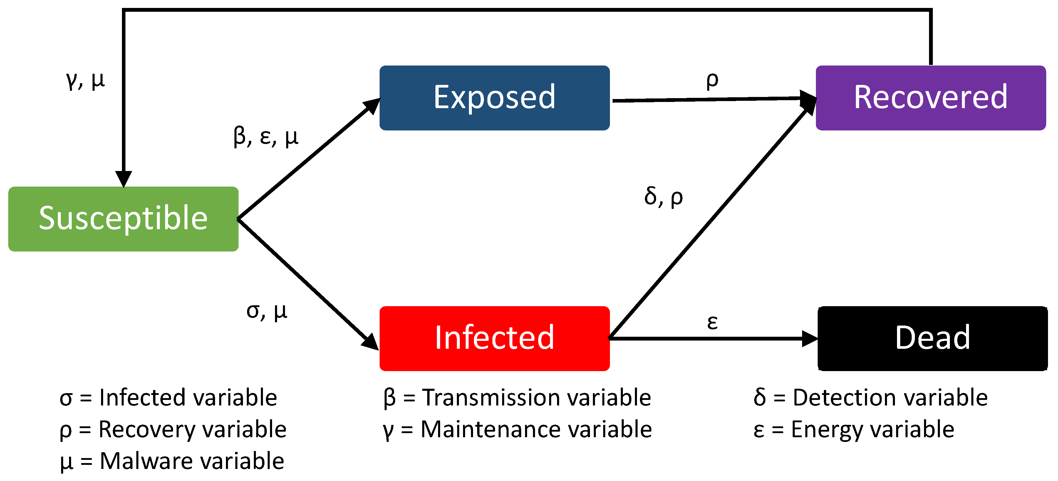
In the proposed SEIRS-D model, the sensor nodes can adopt, in each instant of time
t, one of the following states (see
Figure 1):
Susceptible: the sensor has not been infected by malware, but they have the computational characteristics to be infected.
Exposed: the sensor reached by malware but, they are not able to transmit malware to neighbour sensor due to the characteristics of those sensors and malware.
Infected: the sensor that has been infected by malware. This infected sensor may have the ability to make infection attempts to its neighbours.
Recovered: the sensor that acquires temporal immunity when malware has been successfully removed or security fixes have been installed.
Dead: the sensor that dies because their power has quickly depleted when they have been infected by malware, physical damage or battery life out
It is supposed that the population of nodes remains constant, consequently: at each step of time t. For a given time t, N is the total number of agents, stands for the number of susceptible agents, represents the number of agents in exposed state, are the infectious agents, denotes the agents in the recovered state and, finally, is the total number of agents in dead state.
Agents are autonomous and heterogeneous entities that can interact with both each other and the environment, according to the transition rules. In the model proposed in this study, these agents are the actors that will be defined in
Section 3.1. The environment of agents represents the simulated virtual world in which agents exist. Moreover, the coefficients determine the characteristics associated with each agent; these coefficients will be described in
Section 3.2. Finally, the behaviour of agents is established by rules that define the response of the agents to environment changes and relations with other agents. In
Section 3.3 these transition rules will be detailed.
3.1. Agents
Six main agents compose the SEIRS-D agent-based model—sensor nodes, malware, network topology, the phenomenon of interest, human action and devices. These agents have been selected after analysing the different environments and characteristics that may be present while a wireless sensor network is working. The main features considered for each agent are the following: (1) importance of participation level in the network, and (2) contribution to the malware infection process.
In
Table 1, the
j-th type agents have labelled by
, the characteristics associated to these agents have indexed by
, the values that these characteristic can assume are denoted by
q, and finally, the probabilities associated to these values have been expressed by
such that
for each
k. For example, the probability that a certain sensor has low (
) computational capacity (
) is
such that
.
Therefore, the agents with their specific characteristics, their corresponding values and probabilities are describes as follows:
Sensor nodes: are responsible for collecting data directly from the environment, being the principal element within the WSN. As a consequence, we will consider the following seven characteristics of sensors nodes:
Type of sensor: sensor, sink and cluster-head nodes are the types of sensors that can be part of the network, as well as the technical specifications that allow each node to perform different functions.
Computational capacity: it has been classified as high and low. A node with high capacity can have a general-purpose processor, static memory, batteries as a power source, a sensor and an internal wireless antenna. A node with low capacity can have a processor with special functions, dynamic memory, solar cells as a power source, multiple sensors and an external wireless antenna.
Energy consumption: may vary between very high and very low.
Capacity of transmission and reception of information: is established in high range when the node has external antennas and low range when the node has internal antennas.
Security level: has been classified as high level when it has advanced security methods; medium-level if it uses cryptographic keys, and low level if it does not have security measures.
Data collection method: has been classified in periodicals, external stimulus or requests.
Duty cycle: maybe in the active state when the node takes environmental measurements or transmits data, and in the inactive state while the node wakes up or sleeps.
Malware: is the malicious code designed with functions to penetrate systems, break security policies or transport harmful files. The next three characteristics of malware are considered in our model:
- 8
Type of malware: such as viruses, worms, trojans, and others.
- 9
Spreading mechanism: can use self-replication, exploit or through user interaction.
- 10
Target: can be malicious code distribution, information exfiltration or Denial of Service (DoS).
Network topology: it refers to node interconnections within the network. We will consider two characteristics of this agent:
- 11
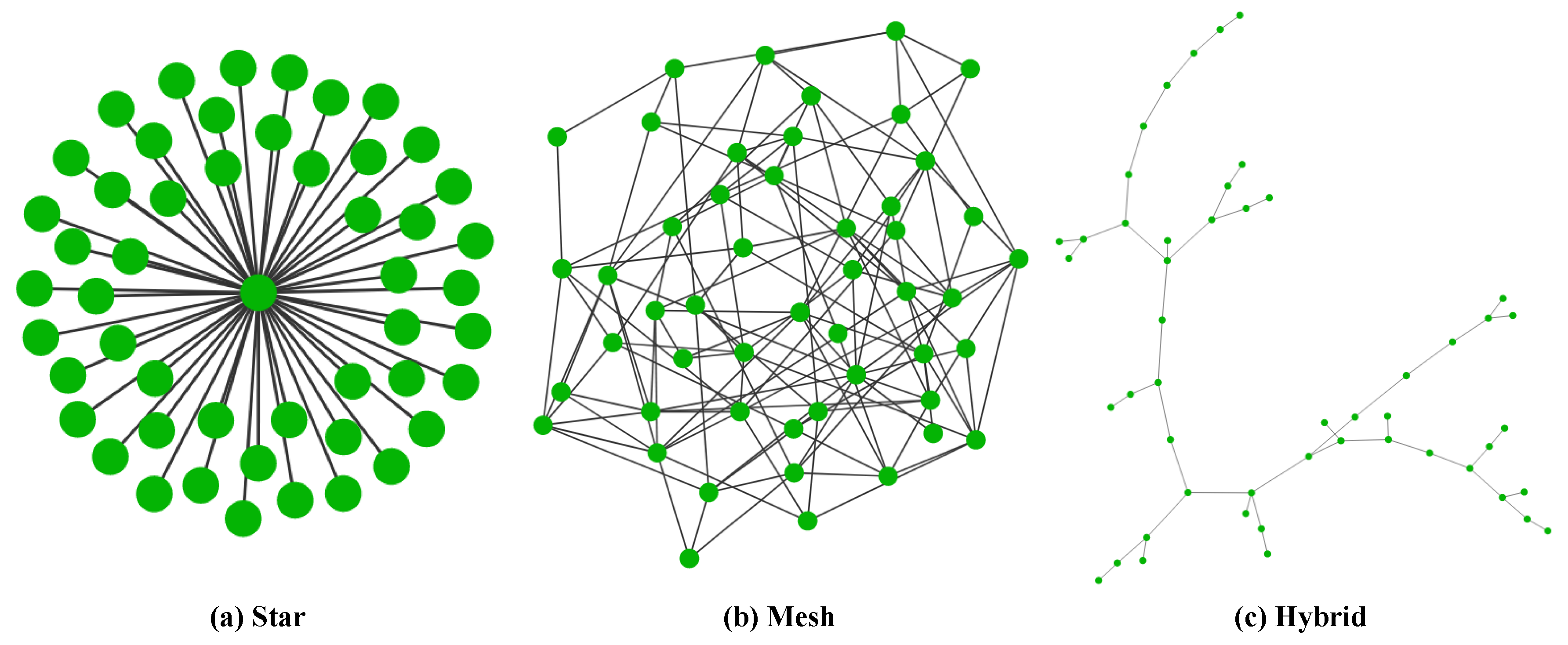
Type of topologies: star topology, mesh topology, and hybrid topology (combination of star topology and mesh topology).
- 12
Routing protocols: most commonly used in WSN are Self-Organizing Protocol (SOP) and Energy Efficient Clustering and Routing (EECR).
Phenomenon of interest: it is directly related to the network environment, so it differs regarding the type and application of the WSN. In this work, we divided the phenomenon by the risk of malware attack occurs, like the following:
- 13
Risk of malware attack: high risk, when the phenomenon is military and industrial phenomena. Medium risk, when the phenomenon is health and environmental phenomena. Moreover, low risk, when the phenomenon is daily activities and multimedia phenomena.
Human action: this is related to the activity level that technicians, administrators, users or attackers may have within the WSN. The only characteristic considered here is:
- 14
Human action level on the network: we have classified in high-level when is related to daily activities or multimedia phenomena; medium level to medicine or environment phenomena, and low-level to the military or industrial phenomena.
Devices: it can be divided into external devices and computing devices. For example, an external device can be a USB flash drive, a memory stick, a CD/DVD and a hard drive. Also, computing devices can be computers, mobile devices, servers and the base station, that is connected to the same network or other networks that have direct communication with WSN. The only characteristic considered is the following:
- 15
Risk of devices infected with malware: we have classified in high risk when the device is infected by malware designed to attack the WSN, medium risk when the devices are infected with malware that cannot attack the WSN, and low risk when the device is not infected with malware.
3.2. Coefficients
In this section, we will describe the coefficients associated with the agents that are involved in the malware propagation process. There are seven coefficients associated with agents, and all of them are probabilities parameters.
3.2.1. Infection Coefficient
This coefficient defines the probability that malware may compromise a susceptible sensor. In this case, the computational characteristics of a sensor will define the probability that it will be infected by the malware designed to attack the WSN. This coefficient depends on the characteristics of the agents defined in the model; however, it can only affect the sensor agents. Consequently, it will be used in the transition rules to define the compartment state of each sensor.
The infection coefficient of the
i-th sensor agent at step of time
t is represented mathematically by
where
and
n is the total number of sensors. As a consequence, the probability that the susceptible
i-th sensor agent will be infected at time
is given by the following coefficient:
where
is a vector defining the characteristics on which depends the variable
. As a consequence the probability of infection depends on the 5 factors:
and
.
represents the characteristics of the sensors,
considers the characteristics of the malware,
are the characteristics of the network topology,
reflects the characteristics of the phenomenon of interest,
represents the characteristics of human action, and
considers the characteristics of the devices. The variable
has not been considered because the network topology can be directly affected the transmission of malware from a sensor to its neighbours due to the interconnections between neighbour nodes.
The risk of infection can be calculated using the probabilities
associated to each possible value of the characteristics of agents (see
Table 1). As a consequence if
with
, we can state the following:
where
q is the value associated to the characteristic
in each case.
In this sense, for each variable the characteristics with the most considerable influence on the infection process have been selected. For this, different scenarios have been studied in order to determine the possible values that allow the risk of infection to be high, medium or low. For example, a military or industrial environment (where human intervention on the network is low and is more likely to be targeted by attackers) may have a high risk of infection if the following conditions are satisfied:
The variable
depends on
such that
since values
and 1 are considered for
respectively.
The variable
depends on
such that
since values
and 3 are considered for
respectively.
The variable
depends on
such that
since the value
is considered for
.
The variable
depends on
such that
since the value
is considered for
.
The variable
depends on
such that
since the value
is considered for
.
3.2.2. Transmission Coefficient
This coefficient refers to the probability that an infected sensor will transmit malware to its susceptible neighbouring sensors. The propagation of malware on a network depends fundamentally on the ability to transfer malware from one node to another. The computational characteristics of each sensor determine this capacity. This coefficient is useful for studying the conditions that must be met for malware to spread.
The transmission coefficient of
i-th sensor agent at the step of time
t is represented mathematically by
where
and
n is the total number of sensors. As a consequence, the probability that an infected
i-th sensor agent will transmit malware at time
is given by the following coefficient:
where
is a vector representing the features on which depends the variable
. The factors
and
determine the probability of transmission. In this case,
,
y
have not been considered because the phenomenon of interest, human action and devices do not directly influence the transmission of malware from one sensor to another, as these factors are neither physical nor logical part of the network.
The risk of transmission can be determined using the Equation (
2); For example, a network with high computational capacity nodes, a low-security level, mesh topology that allows all nodes to communicate with each other and also uses the EECR protocol, may have a higher risk that the sensors will be able to transmit malware to other sensors if the following conditions are fulfilled:
The variable
depends on
such that
since values
and 1 are considered for
respectively.
The variable
depends on
such that
since values
and 3 are considered for
respectively.
The variable
depends on
such that
since the value
is considered for
.
3.2.3. Detection Coefficient
This coefficient refers to the probability that malware in the infected sensor will be detected. The detection time of the malware may be higher or less according to the effects of the phenomenon of interest on the duty cycle and useful battery life. Besides, an infected sensor may receive maintenance that could increase the probability of malware will be detected.
The detection coefficient of the
i-th sensor agent at the step of time
t is represented mathematically by
where
and
n is the total number of sensors. As a result, the probability that the malware will be detected in an infected
at time
is given by the following coefficient:
where
is a vector describing the characteristics on which depends the variable
. The factors
,
and
have not been considered in this coefficient due to malware, topology and devices do not directly influence the detection of malware in an infected sensor, because discovery is performed through alerts generated by security mechanisms or by network administrators at the time of maintenance on the sensors. The risk of detection can be evaluated using the Equation (
2).
For instance, a network with sensors of high computational capacity, a high level of security and where the phenomenon of interest allows the system to be frequently monitored by network administrators, are more likely to detect a malware that has infected a sensor if following conditions are successful:
The variable
depends on
such that
since values
and 3 are considered for
respectively.
The variable
depends on
such that
since the value
is considered for
.
The variable
depends on
such that
since the value
is considered for
.
3.2.4. Recovery Coefficient
This coefficient indicates the probability that a sensor will acquire temporary immunity after the malware has been appropriately removed or the sensor has been serviced. When a sensor has been recovered, it is likely to return to its normal operating state. Finally, when the malware has been removed from the whole network, the recovered sensor becomes susceptible.
The recovery coefficient of
i-th sensor agent is represented mathematically by
where
and
n is the total number of sensors, in the step of time
t. As a consequence, the following coefficient gives the probability that an infected
i-th sensor agent will recover at time
is given by the following coefficient:
where
is a vector specifying the features on which depends the variable
. The following factors have not been considered,
because the malware must have been removed for the sensor to have recovered status,
and
because the phenomenon of interest and devices do not influence the recovery process. The risk of recovery can be determined using the Equation (
2). Such as a network with sensors of high computational capacity, hybrid topology, and higher human action, the sensors are more likely to be able to recover from infection if the following conditions are met:
The variable
depends on
such that
since the value
is considered for
.
The variable
depends on
such that
since values
and 2 are considered for
respectively.
The variable
depends on
such that
since the value
is considered for
.
3.2.5. Maintenance Coefficient
This coefficient indicates the probability that the network administrators will perform the maintenance of a sensor. Support can be both software (e.g., updates of operating systems, antivirus or other security measures), and hardware changes (for example, a replacement for the power source).
The maintenance coefficient of
i-th sensor agent at the step of time
t is represented mathematically by
where
and
n is the total number of sensors. Consequently, the probability that an infected
i-th sensor agent will receive the maintenance at time
is given by the following coefficient:
where
is a vector determining the characteristics on which depends the variable
. The factors that have not been considered in this coefficient are
because there is no relationship between malware and maintenance, whose objective of maintenance is to prevent the network from being infected;
because the phenomenon of interest is independent of maintenance, since it can receive to a greater or lesser degree of support according to human action; and
because external devices do not belong directly to the network.
The risk of maintenance can be computed using the Equation (
2); In particular, a network where the sensors have a high energy consumption, and human intervention in the system is high, is more likely to perform maintenance to the sensors if the following conditions are complied with:
The variable
depends on
such that
since the value
is considered for
.
The variable
depends on
such that
since the value
is considered for
.
The variable
depends on
such that
since the value
is considered for
.
3.2.6. Energy Coefficient
It indicates whether a sensor has the minimum power to continue its normal operational functions. Typically, the energy level of a sensor decreases as time goes on its duty cycle, and it may increase when network administrators or technicians perform maintenance procedures. However, the energy level of a node can drop dramatically when the node has been infected by malware.
The energy coefficient of
i-th sensor agent is represented mathematically by
where
and
n is the total number of sensors, in the step of time
t. Subsequently, the probability that a
i-th sensor agent has the energy to continue its regular operation at time
is given by the following coefficient:
where
is a vector denoting the features on which depends the variable
. The factor
has been selected because the energy level of sensors is related to the functions performed by each node in the network.
For example, a sensor with low energy consumption at every time
t is more likely to conserve an optimal energy level over a long period. The risk of energy can be representing using the equation (
2); The following conditions must be fulfilled:
The variable
depends on
such that
since the value
is considered for
.
3.2.7. Malware Coefficient
This coefficient indicates whether malware has been designed to attack a WSN. This malware can have different targets and types of attack; however, it must be able to infect a sensor considering the operating system and the computational capacity of the sensors that are usually lower than the capabilities of a computer.
The malware coefficient of
i-th sensor agent at the step of time
t is represented mathematically by
where
and
n is the total number of malware. As a result, the probability that
i-th sensor agent will be designed for WSN attack at time
is given by the following coefficient:
where
is a vector defining the characteristics on which depends the variable
. The factor
has been selected in this coefficient because it identifies the essential characteristics that a malware designed for WSN may have. The risk of malware can be computed using the Equation (
2); for example, the probability of WSN infection increases when malware has been designed specifically for attacks on WSN-type networks, for which the following conditions must be present:
The variable
depends on
such that
since the value
is considered for
.
3.3. Transitions Rules
The transition rules of the SEIRS-D model define the conditions that a sensor must be satisfied to change from one state to another in a step of time t, where the state of . The conditions of these rules are based on previously defined coefficients.
The coefficients that can be applied to the sensor agents are infection, transmission, detection, recovery, maintenance and energy; the malware coefficient can be used to the malware agents. Before using these coefficients in the transition rules, it is necessary to define their boolean values from the probabilities given above, as seen below:
Transition rules define how the sensors interact with each other and their environment. These rules are described next:
3.3.1. Susceptible to Infected
A sensor can move from susceptible to infected state when it is successfully compromised by malware during an attack. The variables related are the infection and malware. The explicit expression is the following:
3.3.2. Susceptible to Exposed
A sensor can get from susceptible to exposed state when it has been infected by malware but does not have the computational capacity to transmit the malware to neighbouring nodes. The variables related are the transmission, energy and malware. That is:
3.3.3. Infection to Dead
During the malware infection, a node can become a dead state when its energy level is low or empty. The variable related is energy. It is supposed that:
3.3.4. Infected to Recovered
A sensor can pass from infected to recovered state when security measures have detected that the node is compromised by malware and it is removed. The typical operational function of the sensor can be recovered. The variables related are the detection and recovery. It is defined as follows:
3.3.5. Exposed to Recovered
A sensor can get from exposed to recovered state when the malware has been detected and removed, and it does not have infected neighbours. The regular operation of the system is recovered. The variable related is the recovery. As a consequence:
3.3.6. Recovered to Susceptible
A sensor can shift from recovered to susceptible state when the malware has been removed from the whole network. However, perfect security does not exist; the system can be attacked by new malware. The variables related are maintenance and malware. Then:
4. Simulation
The simulation of an ABM can be developed in different specialised software, both free as paid software. Each solution provides useful features for different areas in which a study can be conducted. The authors of Reference [
33] presents a comprehensive summary of the tools used to modelling and simulated these models, their area of application, and the analyse between model development ease and the computational modelling capability; another critical feature is the scalability level of the models.
The simulation of the SEIRS-D model has been developed in Mesa Framework [
34]. This framework has been selected based on the number of nodes supported, the implementation area, the programming environment and the visualisation of the results. In this case, a network of 500 nodes, science computer as implementation area, Python as the programming language, the generation of graphics and visualization of results in real-time have been established as minimum requirements for the selection of the simulation tool.
Mesa Framework uses the Apache2 web server and the Python programming language for data analysis. Mesa is an alternative to NetLogo. The models simulated in NetLogo have been replicated in Mesa. This framework has been installed on a Virtual Machine (VM) with Ubuntu Linux 16.4 distribution. The computational resources have been used in the VM are an Intel i5 Processor, 2GB Random Access Memory (RAM), 10GB Hard Disk Drive (HDD) and Internet connection. The installation of the framework has been done through a Linux console, following the user manual.
The simulation of the model was implemented with 500 nodes, each node corresponds to a different type of sensor agents, also, in each phenomenon of interest have been defined three topologies: hybrid, mesh and star (see
Figure 2). The maximum simulation time has been 168 hours, and this is equivalent to one week. Next, the description of each scenario and the results obtained will be presented.
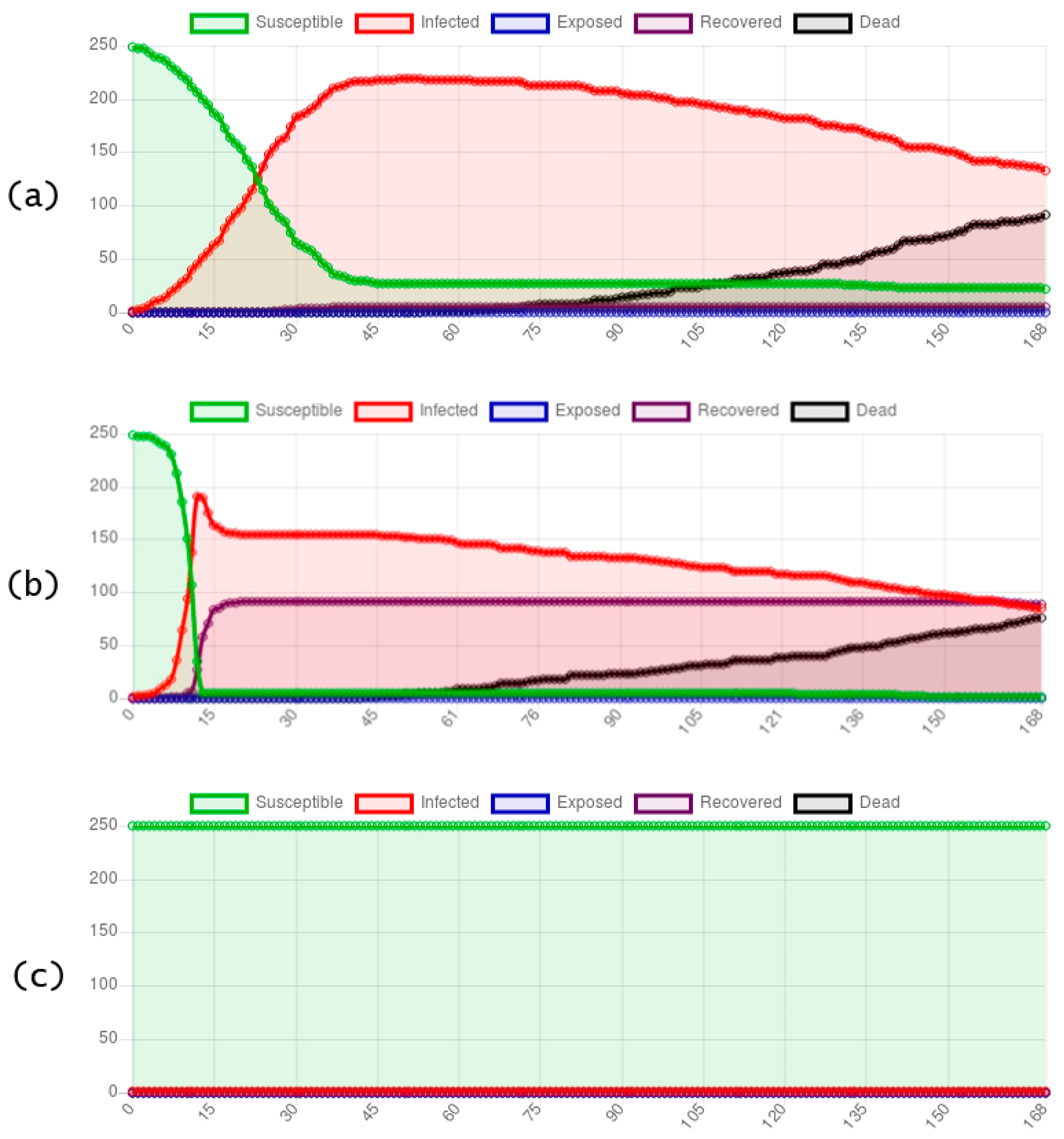
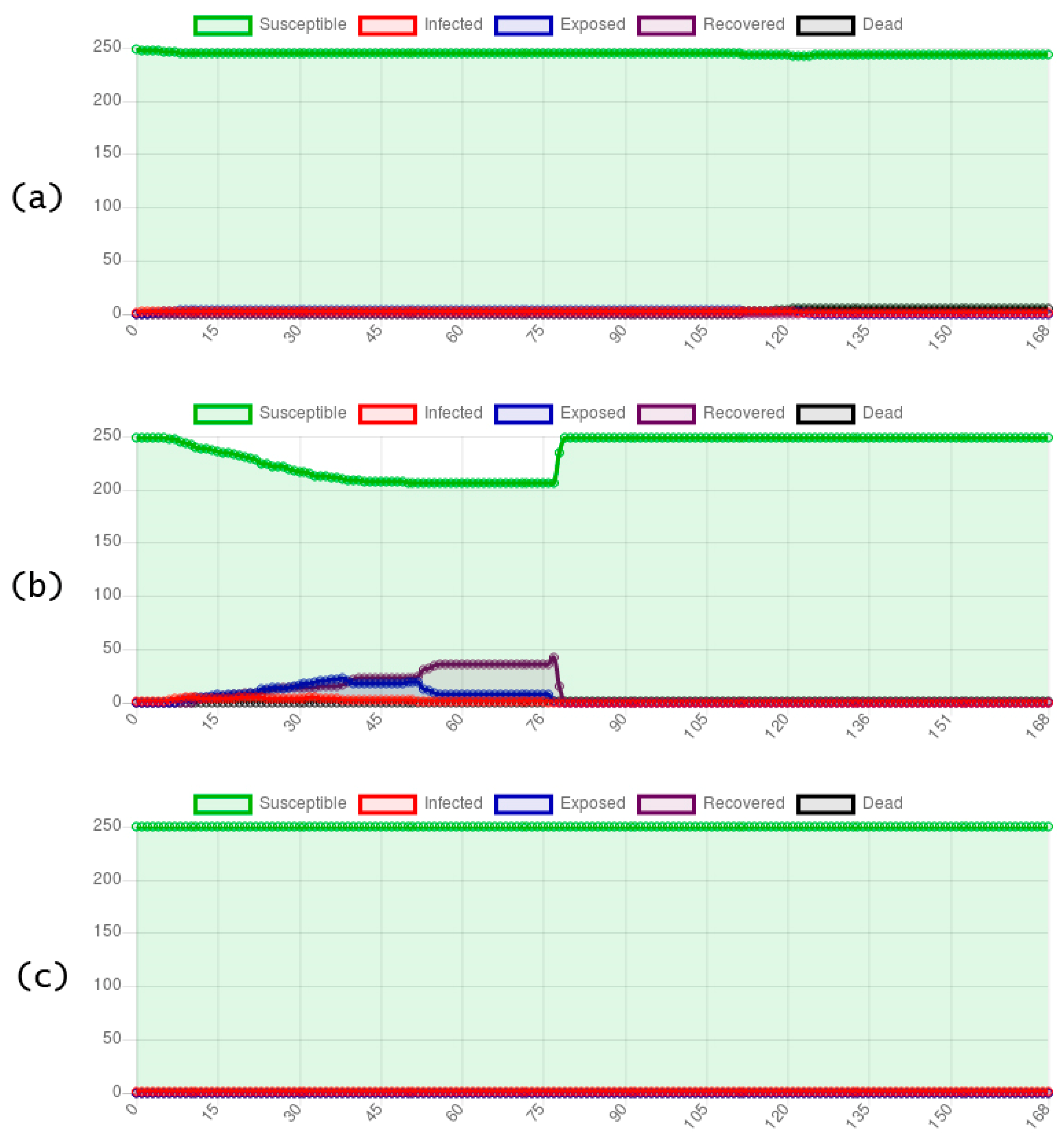
4.1. Scenario 1
In this scenario, the environment is the military and industrial phenomena of interest, malware has been defined with self-replication as a propagation mechanism, and its target is the information infiltration on the network. Besides, the risk of malware attacks is high, the human activity is low, and the risk of infection through devices is medium. Furthermore, the system uses the SOP protocol for node communication, the computational capacity of every node is high, the antenna range of the nodes is high, and the security level of the nodes is from medium to high.
Configurations per topology are the following: (a) Hybrid topology with 98 sensor nodes, 151 router nodes and one sink node. (b) Mesh topology with 249 router nodes and one sink node. (c) Star topology with 249 sensor nodes and one sink node. These simulation parameters have resulted in the following graphs for hybrid (see
Figure 3a), mesh (see
Figure 3b) and star (see
Figure 3c) topologies. The evolution of the compartments of the sensor in each topology is observed.
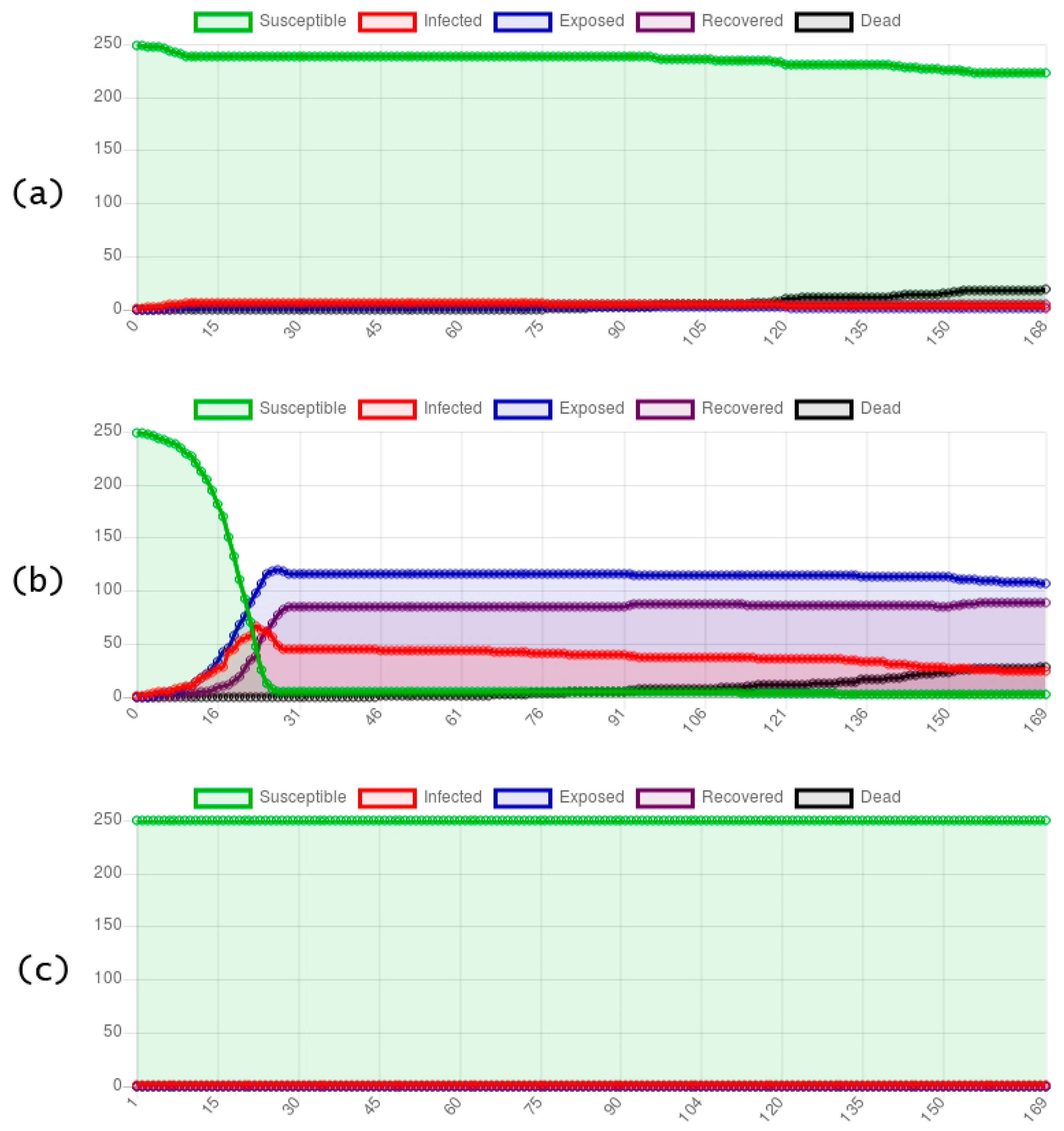
4.2. Scenario 2
The setting for this scenario is the health and environmental phenomena. The graphs of the evolution of the compartments of the sensors in hybrid (see
Figure 4a), mesh (see
Figure 4b) and star (see
Figure 4c) topologies are observed. Parameters are the following: a malware with the exploitation as a propagation mechanism, and its target is Denial of Services. Also, the risk of malware attacks is medium, the human action level is medium, and the risk of infection through devices is low. Also, the network uses the SOP protocol for node communication, the computational capacity of each node is low, the antenna range of the nodes is high, and the security of the nodes is low to medium level.
The following topologies and node types have been defined: (a) Hybrid topology with 89 sensor nodes, 160 router nodes and one sink node. (b) Mesh topology with 249 router nodes and one sink node. (c) Star topology with 249 sensor nodes and one sink node.
4.3. Scenario 3
Finally, an environment has been defined with daily activities and multimedia phenomena. In this case, malware has been defined with user interaction as a propagation mechanism, and its target is network fraud. At the same time, the risk of malware attacks is low, the level of human action is high, and the risk of infection through devices is high. Furthermore, the computational capacity of each node is from low to high, the antenna range of the nodes is between low and high, the safety of the nodes is low or high, and the network uses the EECR protocol for node communication.
The following features have been defined: (a) Hybrid topology with 96 sensor nodes, 153 router nodes and one sink node. (b) Mesh topology with 249 router nodes and one sink node. (c) Star topology with 249 sensor nodes and one sink node. Next, the graphs with the results obtained in this scenario can be seen in (
Figure 5a–c).
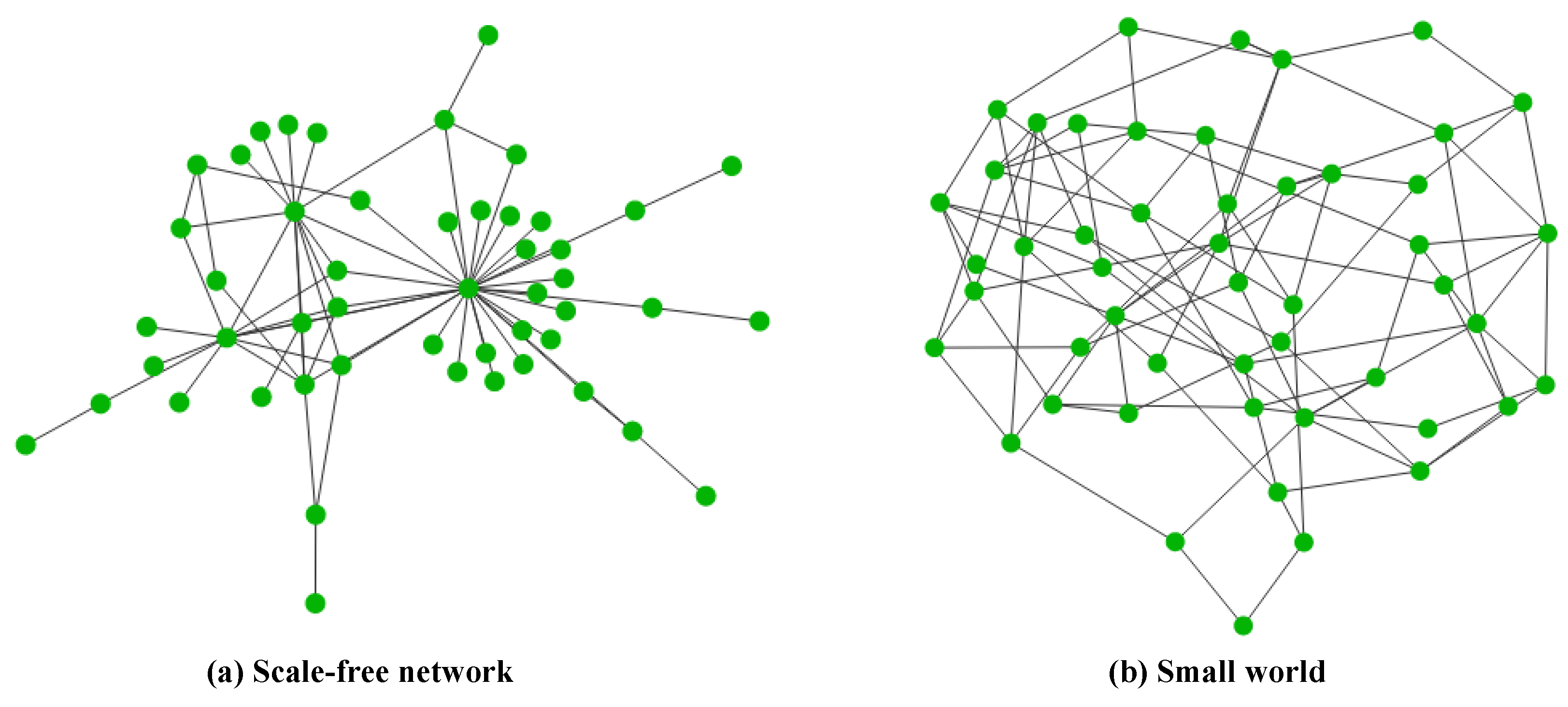
4.4. Complex Networks
The simulation of complex networks has been implemented in the environment of military and industrial phenomena of interest, where malware intends at filtering information and its mechanism of propagation is self-replication. The risk of attack is high, the level of human action is low, and the risk of infection by infected devices is medium. The nodes have antennas with high transmission range, the security level is medium to high, and the computational capacity is high.
A free-scale network and a small world have been configured with a total of 800 nodes (see
Figure 6). These nodes have been distributed as follows: (a) the free-scale network with 461 sensor nodes, 338 router nodes and 1 sink node. (b) The small world with 799 router nodes and 1 sink node.
In the free scale network, three probabilities have been defined, alpha, beta and gamma. The sum of these three probabilities should be equal to 1. Alpha is the probability of adding a new node connected to an existing node that has been randomly selected according to the in-grade distribution; this probability has been assigned a value of 0.41. Beta is defined as the probability of adding an edge between two existing nodes, where one existing node has been randomly selected according to the in-grade distribution, and the other node has been randomly selected according to the out-grade distribution. The Beta probability has a value of 0.54. Gamma is the probability of connecting a new node to an existing node; this existing node is randomly chosen according to the out-grade distribution. The Gamma probability has a value of 0.05.
In this case, the bias for choosing nodes in the in-grade distribution is 0.2 and in the out-grade distribution is 0.
The parameters that have been set in the small world are k=4, wherein a ring topology a node is linked with its k-NN, the probability of re-linking each edge is 0.5 and 20 attempts to generate a connected graph.
4.5. Some Ideas about the Complexity of This Model
The performance of this model is not very expensive from the point of view of Computational Complexity. Obviously it depends on the number of agents considered, n, and the total simulation time period T.
Specifically, the computation of the different epidemiological coefficients (infection coefficient, transmission coefficient, detection coefficient, recovery coefficient, maintenance coefficient, energy coefficient and malware coefficient) takes products. On the other hand, a simple calculus shows that the evaluation of the transition rules takes comparisons.
5. Discussion
In this work, an SEIRS-D agent-based model to simulate the spreading of malware on wireless sensor networks is introduced. Agents, coefficients and transition rule have structured this model. Each agent has been classified in one of the following compartments: susceptible, infected, exposed, recovered and dead.
Moreover, the model proposed in this work was based on seven significant coefficients: infection, transmission, detection, recovery, maintenance, energy and malware. Satisfactory results will be obtained if correctly identify such coefficients and then set up the proper transition rules.
The simulation of the proposed model has been executed in three different scenarios that correspond to the phenomenon of interest agent. In each situation, different global values have been established to simulate a real environment. These parameters have been replicated in the three network topology agents. The analysis of the results has been carried out in two categories: by scenario and by topology.
5.1. Results per Scenario
In the first scenario, the simulation has been conducted in military and industrial environment. In this type of networks, the characteristics of the nodes and security of the net tend to be high. Also, the network is not within reach of the attackers; for these reasons, an infection in these networks is complicated. In
Figure 3 is observed that the infection rate is low in hybrid and star topologies; however, in the mesh topology, the infection has spread to a more significant number of sensors.
In the second scenario, the simulation environment has been performed in health and environmental. In these networks, the sensors may have low characteristics, and security levels between low and medium, the network is more accessible to attackers, although with limitations due to its location. In this case, the infection may take a long time to be detected. In
Figure 4 is observed that the infection advances rapidly in the hybrid and mesh topologies; however, in the star topology, the infection is not capable of spreading.
In the third scenario, the simulation has been done in an environment of daily activities and multimedia. In these networks, the characteristics of the nodes are diverse from one sensor to another, for example, the same network can have the sensors with high characteristics and security, and others with low features and security. However, users interact more frequently with these networks, so that updates or infection detection can be done more quickly. In this case, the mesh topology network has been able to recover from an infection in a short step of time. However, in the cases of hybrid and star topologies, the infection has advanced to a few sensors (see
Figure 5).
5.2. Results per Topology
The hybrid topology presents the particularity that the nodes are grouped in small groups called clusters so that the nodes of a cluster communicate directly with the cluster head node. For these reasons, when the cluster head node has the high computational characteristics and security, the propagation of the infection is prevented from spreading its neighbours and remaining only in that part of the network until it is eliminated.
Mesh topology has the highest infection rate. In this network type, all nodes are able to communicate with each other. In this case, the computational and security characteristics of the nodes may contribute to avoid or recover their normal working state, after an infection.
In star topology, all nodes communicate through the sink node. In this case, the infection can spread quickly if the sink node is infected. However, when a sensor node has been infected is probably that the malware is not able to spread to other nodes.
The topology that can facilitate a quick infection is the mesh topology. However, this topology requires many resources to function correctly, so infection with malware can drastically reduce the functionality of the network. The star topology can be considered as difficult to infect, as long as the characteristics of the sink node are high. Finally, the hybrid topology has the advantage that the infection can stop in a small section of the network, avoiding compromising the functionality of the entire system.
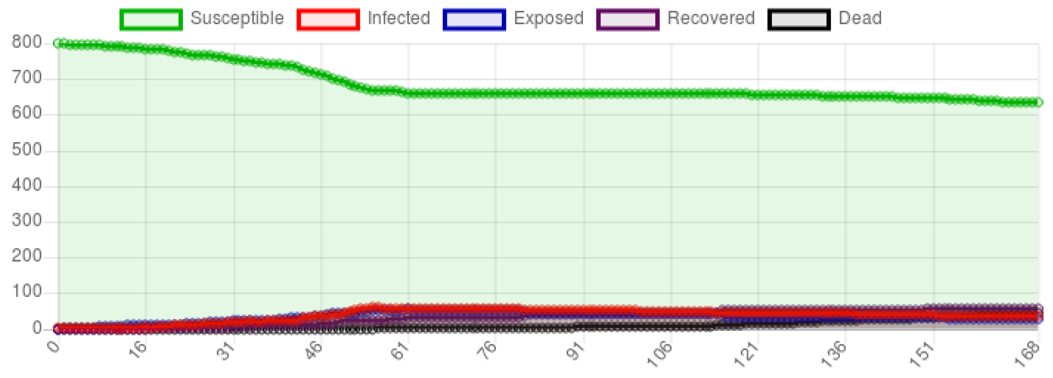
5.3. Results of Complex Networks
In a free-scale network, the number of links in a node is different for each of them. In this case, the spread of the malware has started slowly, then the number of infected nodes and exposed nodes has increased similarly. However, recovery of nodes has started early; therefore, the infection has been able to be controlled quickly, and it has spread in only about 20% of the network (see
Figure 7).
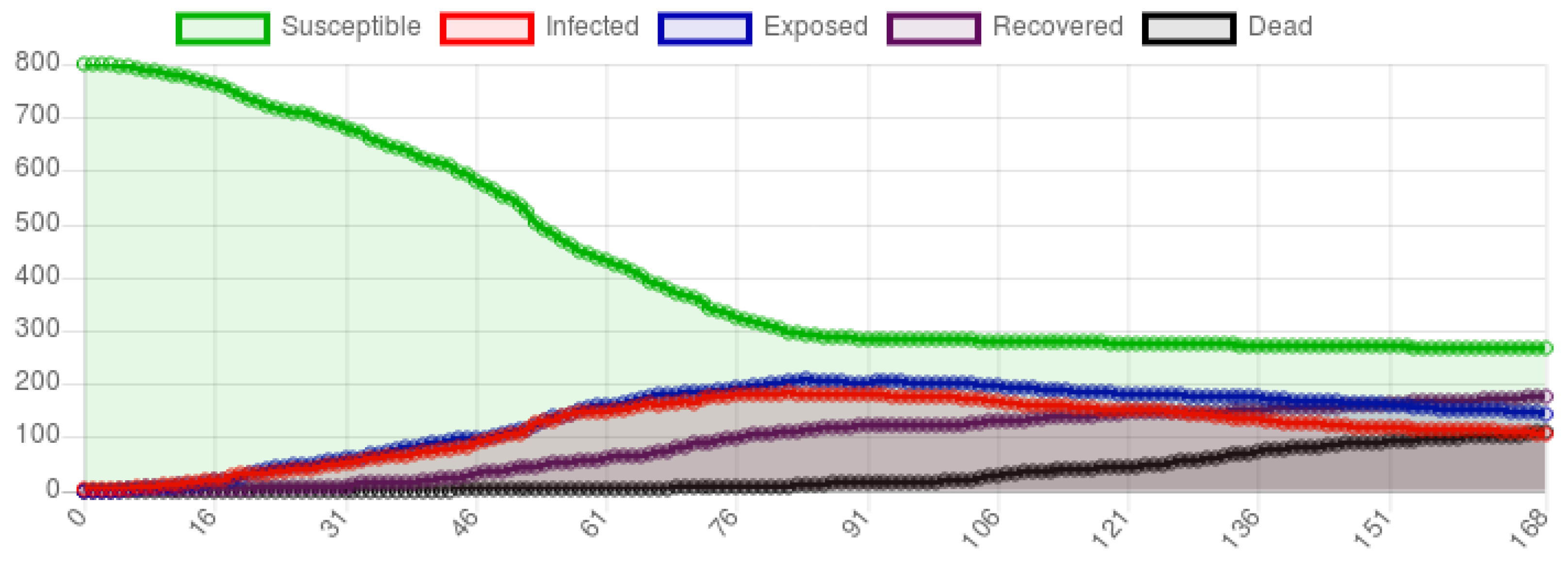
In a small world, two non-neighbouring nodes can communicate with each other, through other neighbouring nodes, with a small number of jumps. In this case, the spread of infection has amplified rapidly, distributed between infected nodes and similarly exposed nodes. When the infection has progressed, the nodes have begun to recover; however, a significant number of infected nodes have started to lose their energy and become dead. In summary, the network can lose data due to intercommunication failures between nodes (see
Figure 8).
6. Conclusions and Future Work
In summary, this model has allowed adjusting the parameters to specific situations, to analyze different results. The analysis of topologies in different environments has contributed to observe the behaviour of malware in more realistic situations; because the agents involved in the model have been carefully selected, considering their most essential characteristics.
The model has been created using the agent-based model paradigm, and it has been based on mathematical epidemiology; furthermore, it has organized in agents, coefficients and transition rules.
The visualization of the results is effortless to understand, and the number of nodes found in the different compartments can be analyzed in each step. The disadvantage of this model has been that no real data has been obtained from a network to analyze other features that may influence the results.
Finally, the results have been confirmed that scenarios and topologies influence the malware propagation process.
The simulation in Mesa Framework has presented limitations in the RAM. The memory has had to be incremented when the number of nodes has increased. Besides, it is necessary to remove the cache from the program because it can fill the hard disk with junk information. Another limitation of this work has been the non-availability of real data for testing in different scenarios.
As future work, the use of machine learning algorithms is proposed as a tool for the simulation and analysis of the proposed model, and this allows the analysis of complex topologies with an efficient use of RAM. Also, the acquisition of a set of data in real scenarios is recommended. Finally, machine learning and data science tools can provide other results with a low error rate.


