Torsion Discriminance for Stability of Linear Time-Invariant Systems

Abstract

This paper extends the former approaches to describe the stability of n-dimensional linear time-invariant systems via the torsion $\tau \left(t\right)$ of the state trajectory. For a system $\dot{r}\left(t\right)=Ar\left(t\right)$ where A is invertible, we show that (1) if there exists a measurable set $E_1$ with positive Lebesgue measure, such that $r\left(0\right)\in E_1$ implies that $\underset{t\to +\infty }{lim}\tau \left(t\right)\ne 0$ or $\underset{t\to +\infty }{lim}\tau \left(t\right)$ does not exist, then the zero solution of the system is stable; (2) if there exists a measurable set $E_2$ with positive Lebesgue measure, such that $r\left(0\right)\in E_2$ implies that $\underset{t\to +\infty }{lim}\tau \left(t\right)=+\infty$, then the zero solution of the system is asymptotically stable. Furthermore, we establish a relationship between the ith curvature $(i=1,2,\cdots )$ of the trajectory and the stability of the zero solution when A is similar to a real diagonal matrix.

1. Introduction

It is well known that Lyapunov [1] laid the foundation of stability theory. Linear systems are the most basic and widely used research objects, which have been developed for a long period. However, the traditional methods rely heavily on linear algebra. There are few results obtained from geometric aspects.

Curvature and torsion are important concepts in differential geometry. In [2], the authors calculated the curvature and torsion of the state trajectories $r\left(t\right)$ of the two- and three-dimensional linear time-invariant systems $\dot{r}\left(t\right)=Ar\left(t\right)$, which are related to the system stability. Furthermore, in [3] the authors use the definition of higher curvatures of curves in ${\mathbb{R}}^n$ given in [4] to obtain the relationship between the first curvature of the state trajectory and the stability of the n-dimensional linear system.

In this paper, we will describe the stability of the zero solutions of linear time-invariant systems in arbitrary dimension by using the torsion, namely, the second curvature.

Our main results are as follows.

Theorem 1.

Suppose that $\dot{r}\left(t\right)=Ar\left(t\right)$ is a linear time-invariant system, where A is similar to an $n\times n$ real diagonal matrix, $r\left(t\right)\in {\mathbb{R}}^n$, and $\dot{r}\left(t\right)$ is the derivative of $r\left(t\right)$. Denote by ${\kappa }_i\left(t\right)(i=1,2,\cdots )$ the ith curvature of trajectory of a solution $r\left(t\right)$. We have

$\left(1\right)$ if there exists a measurable set $E\subseteq {\mathbb{R}}^n$ whose Lebesgue measure is greater than 0, such that $r\left(0\right)\in E$ implies that $\underset{t\to +\infty }{lim}{\kappa }_i\left(t\right)\ne 0$ or $\underset{t\to +\infty }{lim}{\kappa }_i\left(t\right)$ does not exist, then the zero solution of the system is stable;

$\left(2\right)$ if A is invertible, then under the assumptions of $\left(1\right)$, the zero solution of the system is asymptotically stable.

Theorem 2.

Suppose that $\dot{r}\left(t\right)=Ar\left(t\right)$ is a linear time-invariant system, where A is an $n\times n$ invertible real matrix, and $r\left(t\right)\in {\mathbb{R}}^n$. Denote by $\tau \left(t\right)$ the torsion of trajectory of a solution $r\left(t\right)$. We have

$\left(1\right)$ if there exists a measurable set $E_1\subseteq {\mathbb{R}}^n$ whose Lebesgue measure is greater than 0, such that $r\left(0\right)\in E_1$ implies that $\underset{t\to +\infty }{lim}\tau \left(t\right)\ne 0$ or $\underset{t\to +\infty }{lim}\tau \left(t\right)$ does not exist, then the zero solution of the system is stable;

$\left(2\right)$ if there exists a measurable set $E_2\subseteq {\mathbb{R}}^n$ whose Lebesgue measure is greater than 0, such that $r\left(0\right)\in E_2$ implies that $\underset{t\to +\infty }{lim}\tau \left(t\right)=+\infty$, then the zero solution of the system is asymptotically stable.

The paper is organized as follows. In Section 2, we review some basic concepts and propositions. In Section 3, we study the relationship between the ith curvature $(i=1,2,\cdots )$ of the trajectory and the stability of the zero solution of the system when the system matrix is similar to a real diagonal matrix, and we prove Theorem 1. In Section 4, we establish a relationship between the torsion of the trajectory and the stability of the zero solution of the system, and complete the proof of Theorem 2. Two examples are given in Section 5. Finally, Section 6 concludes the paper.

2. Preliminaries

Throughout this paper, all vectors will be written as column vectors, and $\parallel x\parallel$ will denote the Euclidean norm of $x={(x_1,x_2,\cdots ,x_n)}^{\mathrm{T}}\in {\mathbb{R}}^n$, namely, $\parallel x\parallel =\sqrt{{\sum }_{i=1}^n{x}_i^2}$. The vector $r^{\left(i\right)}\left(t\right)$ denotes the ith derivative of vector $r\left(t\right)$. We denote by $detA$ the determinant of matrix A. The eigenvalues of matrix A are denoted by ${\lambda }_i\left(A\right)(i=1,2,\cdots ,n)$, and the set of eigenvalues of matrix A is denoted by $\sigma \left(A\right)$. The degree of polynomial $f\left(t\right)$ is denoted by $deg\left(f\right(t\left)\right)$.

2.1. Stability of Linear Time-Invariant Systems

Definition 1

([5]). The system of ordinary differential equations

$$\begin{array}{c}\hfill \dot{r}\left(t\right)=Ar\left(t\right)\end{array}$$

(1)

is called a linear time-invariant system, where A is an $n\times n$ real constant matrix, $r\left(t\right)\in {\mathbb{R}}^n$, and $\dot{r}\left(t\right)$ is the derivative of $r\left(t\right)$.

Proposition 1

([5]). The initial value problem

$$\begin{array}{c}\hfill \left\{\begin{array}{cc}\hfill \dot{r}\left(t\right)& =Ar\left(t\right),\hfill \\ \hfill r\left(0\right)& =r_0,\hfill \end{array}\right.\end{array}$$

(2)

has a unique solution given by

$$\begin{array}{c}\hfill r\left(t\right)={\mathrm{e}}^{tA}{r}_0,\end{array}$$

(3)

where ${\mathrm{e}}^{tA}={\sum }_{k=0}^{\infty }\frac{t^k{A}^k}{k!}$.

The curve $r\left(t\right)$ is called the trajectory of the system (2) with the initial value $r_0\in {\mathbb{R}}^n$.

Definition 2

([6,7]). The solution $r\left(t\right)\equiv 0$ of differential equations (1) is called the zero solution of the linear time-invariant system. If for every constant $\epsilon >0$, there exists a $\delta =\delta \left(\epsilon \right)>0$, such that $\parallel r\left(0\right)\parallel <\delta$ implies that $\parallel r\left(t\right)\parallel <\epsilon$ for all $t\in [0,+\infty )$, where $r\left(t\right)$ is a solution of (1), then we say that the zero solution of system (1) is stable. If the zero solution is not stable, then we say that it is unstable.

Suppose that the zero solution of system (1) is stable, and there exists a $\tilde{\delta }(0<\tilde{\delta }⩽\delta )$, such that $\parallel r\left(0\right)\parallel <\tilde{\delta }$ implies that $\underset{t\to +\infty }{lim}r\left(t\right)=0$, then we say that the zero solution of system (1) is asymptotically stable.

Proposition 2

([6]). The zero solution of system (1) is stable if and only if all eigenvalues of matrix A have nonpositive real parts and those eigenvalues with zero real parts are simple roots of the minimal polynomial of A.

The zero solution of system (1) is asymptotically stable if and only if all eigenvalues of matrix A have negative real parts, namely, $\mathrm{Re}\left\{{\lambda }_i\left(A\right)\right\}<0(i=1,2,\cdots ,n)$.

Proposition 3

([6]). Suppose that A and B are two $n\times n$ real matrices, and A is similar to B, namely, there exists an $n\times n$ real invertible matrix P, such that $A=P^{-1}BP$. For system (1), let $v\left(t\right)=Pr\left(t\right)$. Then the system after the transformation becomes

$$\begin{array}{c}\hfill \dot{v}\left(t\right)=Bv\left(t\right).\end{array}$$

(4)

System (4) is said to be equivalent to system (1), and $v\left(t\right)=Pr\left(t\right)$ is called an equivalence transformation.

Proposition 4

([6]). Let A and B be two $n\times n$ real matrices, and A is similar to B. Then the zero solution of the system $\dot{r}\left(t\right)=Ar\left(t\right)$ is (asymptotically) stable if and only if the zero solution of the system $\dot{v}\left(t\right)=Bv\left(t\right)$ is (asymptotically) stable.

2.2. Curvatures of Curves in ${\mathbb{R}}^n$

Definition 3

([8]). Let $r:[0,+\infty )\to {\mathbb{R}}^3$ be a smooth curve. The functions

$$\begin{array}{c}\hfill \kappa \left(t\right)=\frac{∥\dot{r}\left(t\right)\times \ddot{r}\left(t\right)∥}{{∥\dot{r}\left(t\right)∥}^3},\tau \left(t\right)=\frac{\left(\dot{r}\left(t\right),\ddot{r}\left(t\right),\stackrel{⃛}{r}\left(t\right)\right)}{{∥\dot{r}\left(t\right)\times \ddot{r}\left(t\right)∥}^2}\end{array}$$

are called the curvature and torsion of the curve $r\left(t\right)$, respectively.

Gluck [4] gave a definition of higher curvatures of curves in ${\mathbb{R}}^n$, which is a generalization of curvature and torsion. Here we omit the definition of higher curvatures and review their calculation formulas directly.

In this paper, $V_i\left(t\right)$ denotes the i-dimensional volume of the i-dimensional parallelotope with vectors $\dot{r}\left(t\right)$, $\ddot{r}\left(t\right)$, ⋯, $r^{\left(i\right)}\left(t\right)$ as edges, and we have a convention that $V_0\left(t\right)=1$.

Proposition 5

([4]). Let $r:[0,+\infty )\to {\mathbb{R}}^n$ be a smooth curve, and $\dot{r}\left(t\right)\ne 0$ for all $t\in [0,+\infty )$. Suppose that for each $t\in [0,+\infty )$, the vectors $\dot{r}\left(t\right),\ddot{r}\left(t\right),\cdots ,r^{\left(m\right)}\left(t\right)(m⩽n)$ are linearly independent. Then the ith curvature of a curve $r\left(t\right)$ is

$$\begin{array}{c}\hfill {\kappa }_i\left(t\right)=\frac{V_{i-1}\left(t\right)V_{i+1}\left(t\right)}{V_1\left(t\right)V_i^2\left(t\right)}(i=1,2,\cdots ,m-1).\end{array}$$

In [4], according to the definition of the curvatures of curves in ${\mathbb{R}}^n$, we have ${\kappa }_i\left(s\right)⩾0$ for $i=1,2,\cdots ,m-1$.

If $r\left(t\right)$ is a smooth curve in ${\mathbb{R}}^3$, and $\dot{r}\left(t\right),\ddot{r}\left(t\right),\stackrel{⃛}{r}\left(t\right)$ are linearly independent, then we have Frenet-Serret formulas (cf. [8]), where ${\kappa }_1\left(s\right)=\kappa \left(s\right)$, and ${\kappa }_2\left(s\right)=\left|\tau \left(s\right)\right|$, which means the first and second curvature are the generalization of curvature and torsion of curves in ${\mathbb{R}}^3$, respectively. In the remainder of this paper, we use $\kappa \left(t\right)$ instead of ${\kappa }_1\left(t\right)$, and $\tau \left(t\right)$ instead of ${\kappa }_2\left(t\right)$, for simplicity.

We can give $V_i\left(t\right)$ by the derivatives of $r\left(t\right)$ with respect to t. In fact, we have the following result.

Proposition 6

([3]). Write $r^{\left(i\right)}\left(t\right)={\left(r_1^{\left(i\right)}\left(t\right),r_2^{\left(i\right)}\left(t\right),\cdots ,r_n^{\left(i\right)}\left(t\right)\right)}^{\mathrm{T}}$. We have

$$\begin{array}{c}\hfill V_k^2\left(t\right)=\sum _{1⩽i_1<i_2<\cdots <i_k⩽n}{\left|\begin{array}{cccc}{\dot{r}}_{i_1}\left(t\right)& {\ddot{r}}_{i_1}\left(t\right)& \cdots & r_{i_1}^{\left(k\right)}\left(t\right)\\ {\dot{r}}_{i_2}\left(t\right)& {\ddot{r}}_{i_2}\left(t\right)& \cdots & r_{i_2}^{\left(k\right)}\left(t\right)\\ ⋮& ⋮& \ddots & ⋮\\ {\dot{r}}_{i_k}\left(t\right)& {\ddot{r}}_{i_k}\left(t\right)& \cdots & r_{i_k}^{\left(k\right)}\left(t\right)\end{array}\right|}^2.\end{array}$$

By Proposition 5 and Proposition 6, we obtain the expression of each curvature of curve $r\left(t\right)$ in ${\mathbb{R}}^n$ by the coordinates of derivatives of $r\left(t\right)$. In particular, if $\dot{r}\left(t\right)$ and $\ddot{r}\left(t\right)$ are linearly independent, then the torsion of $r\left(t\right)$ satisfies

$$\begin{array}{c}\hfill \tau \left(t\right)=\frac{V_3\left(t\right)}{V_2^2\left(t\right)}=\frac{\sqrt{{\sum }_{1⩽i<j<k⩽n}{\left|\begin{array}{ccc}{\dot{r}}_i\left(t\right)& {\ddot{r}}_i\left(t\right)& {\stackrel{⃛}{r}}_i\left(t\right)\\ {\dot{r}}_j\left(t\right)& {\ddot{r}}_j\left(t\right)& {\stackrel{⃛}{r}}_j\left(t\right)\\ {\dot{r}}_k\left(t\right)& {\ddot{r}}_k\left(t\right)& {\stackrel{⃛}{r}}_k\left(t\right)\end{array}\right|}^2}}{{\sum }_{1⩽p<q⩽n}{\left|\begin{array}{cc}{\dot{r}}_p\left(t\right)& {\ddot{r}}_p\left(t\right)\\ {\dot{r}}_q\left(t\right)& {\ddot{r}}_q\left(t\right)\end{array}\right|}^2}.\end{array}$$

(5)

On the other hand, if $V_2\left(t\right)\equiv 0$, namely $\dot{r}\left(t\right)$ and $\ddot{r}\left(t\right)$ are linearly dependent for all t, then obviously we have the convention that $\tau \left(t\right)\equiv 0$. Further, the function $V_2\left(t\right)$ will be examined in detail in Section 4.2.

2.3. Relationship Between the Curvatures of Two Equivalent Systems

Wang et al. [3] establish a relationship between the curvatures of the trajectories of two equivalent systems. In fact, let a curve $r\left(t\right)$ be the trajectory of system (2), and suppose that for each t, the vectors $\dot{r}\left(t\right),\ddot{r}\left(t\right),\cdots ,r^{\left(m\right)}\left(t\right)$ are linearly independent. Then we can define curvatures ${\kappa }_{r,1}\left(t\right),{\kappa }_{r,2}\left(t\right),\cdots ,{\kappa }_{r,m-1}\left(t\right)$ of the curve $r\left(t\right)$, and we have the following result.

Proposition 7

([3]). Suppose that a linear time-invariant system $\dot{r}\left(t\right)=Ar\left(t\right)$ is equivalent to a system $\dot{v}\left(t\right)=Bv\left(t\right)$, where $A=P^{-1}BP$, and $v\left(t\right)=Pr\left(t\right)$ is the equivalence transformation. Let ${\kappa }_{r,i}\left(t\right)$ and ${\kappa }_{v,i}\left(t\right)$ be the ith $(i=1,2,\cdots ,m-1)$ curvatures of trajectories $r\left(t\right)$ and $v\left(t\right)$, respectively. Then we have

$$\begin{array}{cc}\hfill \underset{t\to +\infty }{lim}{\kappa }_{r,i}\left(t\right)=0& ⟺\underset{t\to +\infty }{lim}{\kappa }_{v,i}\left(t\right)=0,\hfill \\ \hfill \underset{t\to +\infty }{lim}{\kappa }_{r,i}\left(t\right)=+\infty & ⟺\underset{t\to +\infty }{lim}{\kappa }_{v,i}\left(t\right)=+\infty ,\hfill \\ \hfill {\kappa }_{r,i}\left(t\right)\mathit{is}a\mathit{bounded}\mathit{function}& ⟺{\kappa }_{v,i}\left(t\right)\mathit{is}a\mathit{bounded}\mathit{function}.\hfill \end{array}$$

2.4. Real Jordan Canonical Form

Proposition 8

([7,9]). Let A be an $n\times n$ real matrix. Then A is similar to a block diagonal real matrix

$$\begin{array}{c}\hfill \left(\begin{array}{ccc}\begin{array}{cc}{C}_{n_1}(a_1,b_1)& \\ & C_{n_2}(a_2,b_2)\\ & & \ddots \end{array}& & 0\\ & C_{n_p}(a_p,b_p)\\ 0& & \begin{array}{cc}{J}_{n_{p+1}}\left({\lambda }_{p+1}\right)& \\ & \ddots \\ & & J_{n_r}\left({\lambda }_r\right)\end{array}\end{array}\right),\end{array}$$

(6)

where

$\left(1\right)$ for $k\in \{1,2,\cdots ,p\}$, the numbers ${\lambda }_k=a_k+\sqrt{-1}{b}_k$ and ${\overline{\lambda }}_k=a_k-\sqrt{-1}{b}_k$ $(a_k,b_k\in \mathbb{R},\mathrm{and}{b}_k>0)$ are complex eigenvalues of A, and

$$\begin{array}{c}\hfill C_{n_k}(a_k,b_k)={\left(\begin{array}{ccccc}{\Lambda }_k& I_2& & & \\ & {\Lambda }_k& I_2& & \\ & & {\Lambda }_k& \ddots & \\ & & & \ddots & I_2\\ & & & & {\Lambda }_k\end{array}\right)}_{2n_k\times 2n_k},\end{array}$$

where ${\Lambda }_k=\left(\begin{array}{cc}{a}_k& b_k\\ -b_k& a_k\end{array}\right),I_2=\left(\begin{array}{cc}1& 0\\ 0& 1\end{array}\right);$

$\left(2\right)$ for $j\in \{p+1,p+2,\cdots ,r\}$, the number ${\lambda }_j$ is a real eigenvalue of A, and

$$\begin{array}{c}\hfill J_{n_j}\left({\lambda }_j\right)={\left(\begin{array}{ccccc}{\lambda }_j& 1& & & \\ & {\lambda }_j& 1& & \\ & & {\lambda }_j& \ddots & \\ & & & \ddots & 1\\ & & & & {\lambda }_j\end{array}\right)}_{n_j\times n_j}.\end{array}$$

The matrix (6) is called the real Jordan canonical form of A.

3. Real Diagonal Matrix

In this section, we study the case that the system matrix is similar to a real diagonal matrix, and prove Theorem 1. From Proposition 4 and Proposition 7, we only need to focus on the case that A is a real diagonal matrix, and prove Proposition 9.

In what follows, we defind a subset of ${\mathbb{R}}^n$ that

$$\begin{array}{c}\hfill S=\left\{r\left(0\right)|r\left(0\right)={(r_1\left(0\right),r_2\left(0\right),\cdots ,r_n\left(0\right))}^{\mathrm{T}}\in {\mathbb{R}}^n,\mathrm{s}.\mathrm{t}.\prod _{i=1}^n{r}_i\left(0\right)\ne 0\right\}.\end{array}$$

Proposition 9.

Suppose that $\dot{r}\left(t\right)=Ar\left(t\right)$ is a linear time-invariant system, where A is an $n\times n$ real diagonal matrix, and $r\left(t\right)\in {\mathbb{R}}^n$. Denote by ${\kappa }_i\left(t\right)(i=1,2,\cdots )$ the ith curvature of trajectory of a solution $r\left(t\right)$. Then for any given initial value $r\left(0\right)\in S$, we have

$\left(1\right)$ if $\underset{t\to +\infty }{lim}{\kappa }_i\left(t\right)\ne 0$ or $\underset{t\to +\infty }{lim}{\kappa }_i\left(t\right)$ does not exist, then the zero solution of the system is stable;

$\left(2\right)$ if A is invertible, and $\underset{t\to +\infty }{lim}{\kappa }_i\left(t\right)\ne 0$ or $\underset{t\to +\infty }{lim}{\kappa }_i\left(t\right)$ does not exist, then the zero solution of the system is asymptotically stable.

Wang et al. [3] has proved the case of $i=1$. Now we give a complete proof of this proposition.

Proof. 

$\left(1\right)$ Suppose that A is an $n\times n$ real diagonal matrix, namely,

$$\begin{array}{c}\hfill A=\mathrm{diag}\{{\lambda }_1,{\lambda }_2,\cdots ,{\lambda }_n\}.\end{array}$$

Then

$$\begin{array}{c}\hfill A^k=\mathrm{diag}\{{\lambda }_1^k,{\lambda }_2^k,\cdots ,{\lambda }_n^k\},{\mathrm{e}}^{tA}=\mathrm{diag}\{{\mathrm{e}}^{{\lambda }_{1}t},{\mathrm{e}}^{{\lambda }_{2}t},\cdots ,{\mathrm{e}}^{{\lambda }_{n}t}\},\end{array}$$

where $p=1,2,\cdots$. Hence we have

$$\begin{array}{c}r\left(t\right)={\mathrm{e}}^{tA}r\left(0\right)={\left({\mathrm{e}}^{{\lambda }_{1}t}{r}_1\left(0\right),{\mathrm{e}}^{{\lambda }_{2}t}{r}_2\left(0\right),\cdots ,{\mathrm{e}}^{{\lambda }_{n}t}{r}_n\left(0\right)\right)}^{\mathrm{T}},\hfill \\ \dot{r}\left(t\right)=Ar\left(t\right)={\left({\lambda }_1{\mathrm{e}}^{{\lambda }_{1}t}{r}_1\left(0\right),{\lambda }_2{\mathrm{e}}^{{\lambda }_{2}t}{r}_2\left(0\right),\cdots ,{\lambda }_n{\mathrm{e}}^{{\lambda }_{n}t}{r}_n\left(0\right)\right)}^{\mathrm{T}},\hfill \\ \cdots \cdots ,\hfill \\ r^{\left(k\right)}\left(t\right)=A^{k}r\left(t\right)={\left({\lambda }_1^k{\mathrm{e}}^{{\lambda }_{1}t}{r}_1\left(0\right),{\lambda }_2^k{\mathrm{e}}^{{\lambda }_{2}t}{r}_2\left(0\right),\cdots ,{\lambda }_n^k{\mathrm{e}}^{{\lambda }_{n}t}{r}_n\left(0\right)\right)}^{\mathrm{T}},\hfill \end{array}$$

namely, the coordinates of derivatives of $r\left(t\right)$ are

$$\begin{array}{c}\hfill {\dot{r}}_i\left(t\right)={\lambda }_i{\mathrm{e}}^{{\lambda }_{i}t}{r}_i\left(0\right),\cdots \cdots ,r_i^{\left(k\right)}\left(t\right)={\lambda }_i^k{\mathrm{e}}^{{\lambda }_{i}t}{r}_i\left(0\right)(i=1,2,\cdots ,n).\end{array}$$

Then by Proposition 6, we obtain

$$\begin{array}{cc}\hfill V_k^2\left(t\right)& =\sum _{1⩽i_1<i_2<\cdots <i_k⩽n}{\left|\begin{array}{cccc}{\dot{r}}_{i_1}\left(t\right)& {\ddot{r}}_{i_1}\left(t\right)& \cdots & r_{i_1}^{\left(k\right)}\left(t\right)\\ {\dot{r}}_{i_2}\left(t\right)& {\ddot{r}}_{i_2}\left(t\right)& \cdots & r_{i_2}^{\left(k\right)}\left(t\right)\\ ⋮& ⋮& \ddots & ⋮\\ {\dot{r}}_{i_k}\left(t\right)& {\ddot{r}}_{i_k}\left(t\right)& \cdots & r_{i_k}^{\left(k\right)}\left(t\right)\end{array}\right|}^2\hfill \\ & =\sum _{1⩽i_1<i_2<\cdots <i_k⩽n}{\left|\begin{array}{cccc}{\lambda }_{i_1}{\mathrm{e}}^{{\lambda }_{i_1}t}{r}_{i_1}\left(0\right)& {\lambda }_{i_1}^2{\mathrm{e}}^{{\lambda }_{i_1}t}{r}_{i_1}\left(0\right)& \cdots & {\lambda }_{i_1}^k{\mathrm{e}}^{{\lambda }_{i_1}t}{r}_{i_1}\left(0\right)\\ {\lambda }_{i_2}{\mathrm{e}}^{{\lambda }_{i_2}t}{r}_{i_2}\left(0\right)& {\lambda }_{i_2}^2{\mathrm{e}}^{{\lambda }_{i_2}t}{r}_{i_2}\left(0\right)& \cdots & {\lambda }_{i_2}^k{\mathrm{e}}^{{\lambda }_{i_2}t}{r}_{i_2}\left(0\right)\\ ⋮& ⋮& \ddots & ⋮\\ {\lambda }_{i_k}{\mathrm{e}}^{{\lambda }_{i_k}t}{r}_{i_k}\left(0\right)& {\lambda }_{i_k}^2{\mathrm{e}}^{{\lambda }_{i_k}t}{r}_{i_k}\left(0\right)& \cdots & {\lambda }_{i_k}^k{\mathrm{e}}^{{\lambda }_{i_k}t}{r}_{i_k}\left(0\right)\end{array}\right|}^2\hfill \\ & =\sum _{1⩽i_1<i_2<\cdots <i_k⩽n}{\left\{{\mathrm{e}}^{\left({\sum }_{p=1}^k{\lambda }_{i_p}\right)t}\prod _{q=1}^k\left({\lambda }_{i_q}{r}_{i_q}\left(0\right)\right)\left|\begin{array}{ccccc}1& {\lambda }_{i_1}& {\lambda }_{i_1}^2& \cdots & {\lambda }_{i_1}^{k-1}\\ 1& {\lambda }_{i_2}& {\lambda }_{i_2}^2& \cdots & {\lambda }_{i_2}^{k-1}\\ ⋮& ⋮& ⋮& \ddots & ⋮\\ 1& {\lambda }_{i_k}& {\lambda }_{i_k}^2& \cdots & {\lambda }_{i_k}^{k-1}\end{array}\right|\right\}}^2\hfill \\ & =\sum _{1⩽i_1<i_2<\cdots <i_k⩽n}{\mathrm{e}}^{2\left({\sum }_{p=1}^k{\lambda }_{i_p}\right)t}{\left\{\prod _{q=1}^k\left({\lambda }_{i_q}{r}_{i_q}\left(0\right)\right)\prod _{1⩽\alpha <\beta ⩽k}\left({\lambda }_{i_{\beta }}-{\lambda }_{i_{\alpha }}\right)\right\}}^2.\hfill \end{array}$$

(7)

We see that if the eigenvalues ${\lambda }_{i_1},{\lambda }_{i_2},\cdots ,{\lambda }_{i_k}$ of A are non-zero and distinct, then a term of the form $C{\mathrm{e}}^{2\left({\sum }_{p=1}^k{\lambda }_{i_p}\right)t}$ will appear in the expression of $V_k^2\left(t\right)$, where C is a constant depending on the eigenvalues and initial value, and $C>0$.

By Proposition 5, the square of the ith curvature is

$$\begin{array}{c}\hfill {\kappa }_i^2\left(t\right)=\frac{V_{i-1}^2\left(t\right)V_{i+1}^2\left(t\right)}{V_1^2\left(t\right)V_i^4\left(t\right)}(i=1,2,\cdots ,m-1).\end{array}$$

(8)

Now, we consider the limit of ${\kappa }_i\left(t\right)$ as $t\to +\infty$ by comparing the exponents of $\mathrm{e}$ in the numerator and denominator of ${\kappa }_i^2\left(t\right)$. Let ${\Delta }_1$ and ${\Delta }_2$ denote the maximum values of $\alpha$ in the terms of the form ${\mathrm{e}}^{\alpha t}$ in $V_{i-1}^2\left(t\right)V_{i+1}^2\left(t\right)$ and $V_1^2\left(t\right)V_i^4\left(t\right)$, respectively. We define

$$\begin{array}{c}{\lambda }_{\left(1\right)}=max\left\{\sigma \left(A\right)\backslash \left\{0\right\}\right\},\hfill \\ {\lambda }_{\left(2\right)}=max\left\{\sigma \left(A\right)\backslash \left\{0,{\lambda }_{\left(1\right)}\right\}\right\},\hfill \\ \cdots \cdots ,\hfill \\ {\lambda }_{\left(i\right)}=max\left\{\sigma \left(A\right)\backslash \left\{0,{\lambda }_{\left(1\right)},{\lambda }_{\left(2\right)},\cdots ,{\lambda }_{(i-1)}\right\}\right\},\hfill \\ \cdots \cdots \hfill \end{array}$$

Then by (7) and (8), we have

$$\begin{array}{c}\hfill {\Delta }_1=2\sum _{a=1}^{i-1}{\lambda }_{\left(a\right)}+2\sum _{b=1}^{i+1}{\lambda }_{\left(b\right)},{\Delta }_2=2{\lambda }_{\left(1\right)}+4\sum _{c=1}^i{\lambda }_{\left(c\right)}.\end{array}$$

Thus,

$$\begin{array}{c}\hfill {\Delta }_1-{\Delta }_2=2\left({\lambda }_{(i+1)}-{\lambda }_{\left(1\right)}-{\lambda }_{\left(i\right)}\right).\end{array}$$

It follows that

$$\begin{array}{c}\hfill \underset{t\to +\infty }{lim}{\kappa }_i\left(t\right)=0⟺{\Delta }_1<{\Delta }_2⟺{\lambda }_{\left(1\right)}+{\lambda }_{\left(i\right)}>{\lambda }_{(i+1)},\\ \hfill \underset{t\to +\infty }{lim}{\kappa }_i\left(t\right)=C⟺{\Delta }_1={\Delta }_2⟺{\lambda }_{\left(1\right)}+{\lambda }_{\left(i\right)}={\lambda }_{(i+1)},\\ \hfill \underset{t\to +\infty }{lim}{\kappa }_i\left(t\right)=+\infty ⟺{\Delta }_1>{\Delta }_2⟺{\lambda }_{\left(1\right)}+{\lambda }_{\left(i\right)}<{\lambda }_{(i+1)},\end{array}$$

(9)

where C is a positive constant depending on the initial value $r\left(0\right)=r_0(r_j\left(0\right)\ne 0$ for $j=1,2,\cdots ,n)$. Here we notice that for any given real diagonal matrix A, if for a given initial value $r\left(0\right)\in {\mathbb{R}}^n$ that satisfies ${\prod }_{j=1}^n{r}_j\left(0\right)\ne 0$, we have $\underset{t\to +\infty }{lim}{\kappa }_i\left(t\right)=0$ (or $+\infty$, or a constant $C>0$, respectively), then for an arbitrary $r\left(0\right)\in {\mathbb{R}}^n$ satisfying ${\prod }_{j=1}^n{r}_j\left(0\right)\ne 0$, we still have $\underset{t\to +\infty }{lim}{\kappa }_i\left(t\right)=0$ (or $+\infty$, or a constant $\tilde{C}>0$, respectively).

Noting that A is a real diagonal matrix, by Proposition 2, the zero solution of the system (1) is stable if and only if ${\lambda }_i\left(A\right)⩽0(i=1,2,\cdots ,n)$. If the zero solution of the system is unstable, then we have ${\lambda }_{\left(1\right)}>0$, thus ${\lambda }_{\left(1\right)}+{\lambda }_{\left(i\right)}>{\lambda }_{(i+1)}$. By (9), we have $\underset{t\to +\infty }{lim}{\kappa }_i\left(t\right)=0$. In other words, if $\underset{t\to +\infty }{lim}{\kappa }_i\left(t\right)\ne 0$ or $\underset{t\to +\infty }{lim}{\kappa }_i\left(t\right)$ does not exist, then the zero solution of the system is stable.

$\left(2\right)$ Suppose that A is invertible, and $\underset{t\to +\infty }{lim}{\kappa }_i\left(t\right)\ne 0$ or $\underset{t\to +\infty }{lim}{\kappa }_i\left(t\right)$ does not exist. Then 0 is not an eigenvalue of A, and the zero solution of the system is stable. By Proposition 2, the zero solution of the system is asymptotically stable. □

Now, we proceed to the proof of Theorem 1.

Proof of Theorem 1.

Suppose that the linear time-invariant system $\dot{r}\left(t\right)=Ar\left(t\right)$ is equivalent to a system $\dot{v}\left(t\right)=Bv\left(t\right)$, where B is a real diagonal matrix, $A=P^{-1}BP$, and $v\left(t\right)=Pr\left(t\right)$ is the equivalence transformation. They by Proposition 7, we have

$$\begin{array}{c}\hfill \underset{t\to +\infty }{lim}{\kappa }_{r,i}\left(t\right)=0⟺\underset{t\to +\infty }{lim}{\kappa }_{v,i}\left(t\right)=0.\end{array}$$

(10)

We define

$$\begin{array}{c}\hfill \tilde{S}=\left\{P^{-1}v\left(0\right)|v\left(0\right)={(v_1\left(0\right),v_2\left(0\right),\cdots ,v_n\left(0\right))}^{\mathrm{T}}\in {\mathbb{R}}^n,\mathrm{s}.\mathrm{t}.\prod _{i=1}^n{v}_i\left(0\right)\ne 0\right\}.\end{array}$$

Note that we can regard any given $n\times n$ invertible matrix P as an invertible linear transformation $P:{\mathbb{R}}^n\to {\mathbb{R}}^n$, and the Lebesgue measure of ${\mathbb{R}}^n\backslash \tilde{S}$ satisfies

$$\begin{array}{c}\hfill m\left({\mathbb{R}}^n\backslash \tilde{S}\right)=0.\end{array}$$

(11)

If there exists a measurable set $E\subseteq {\mathbb{R}}^n$ whose Lebesgue measure is greater than 0, such that $r\left(0\right)\in E$ implies that $\underset{t\to +\infty }{lim}{\kappa }_{r,i}\left(t\right)\ne 0$ or $\underset{t\to +\infty }{lim}{\kappa }_{r,i}\left(t\right)$ does not exist, then by (10) and (11), there exists a $r\left(0\right)\in \tilde{S}$, such that the trajectory $v\left(t\right)$ with initial value $v\left(0\right)=Pr\left(0\right)$ satisfies $\underset{t\to +\infty }{lim}{\kappa }_{v,i}\left(t\right)\ne 0$ or $\underset{t\to +\infty }{lim}{\kappa }_{v,i}\left(t\right)$ does not exist. Notice that when $r\left(0\right)\in \tilde{S}$, the vector $v\left(0\right)$ satisfies ${\prod }_{i=1}^n{v}_i\left(0\right)\ne 0$, thus by Proposition 9, the zero solution of the system $\dot{v}\left(t\right)=Bv\left(t\right)$ is stable, and then by Proposition 4, the zero solution of the system $\dot{r}\left(t\right)=Ar\left(t\right)$ is also stable, which proves Theorem 1 (1).

Since A is similar to B, the matrix A is invertible if and only if B is invertible. The method of the proof of (1) works for (2), which completes the proof of Theorem 1. □

4. Relationship between Torsion and Stability

In this section, we give the proof of Theorem 2, which establishes a relationship between the torsion of the trajectory and the stability of the zero solution of the system. From Proposition 4, 7, and 8, we only need to focus on the case that A is an invertible matrix in real Jordan canonical form (6), and prove the following result.

Proposition 10.

Suppose that $\dot{r}\left(t\right)=Ar\left(t\right)$ is a linear time-invariant system, where A is an $n\times n$ invertible matrix in real Jordan canonical form, and $r\left(t\right)\in {\mathbb{R}}^n$. Denote by $\tau \left(t\right)$ the torsion of trajectory of a solution $r\left(t\right)$. Then for any given initial value $r\left(0\right)\in S$, we have

$\left(1\right)$ if $\underset{t\to +\infty }{lim}\tau \left(t\right)\ne 0$ or $\underset{t\to +\infty }{lim}\tau \left(t\right)$ does not exist, then the zero solution of the system is stable;

$\left(2\right)$ if $\underset{t\to +\infty }{lim}\tau \left(t\right)=+\infty$, then the zero solution of the system is asymptotically stable.

4.1. Blocks $J_p\left(\lambda \right)$ and $C_m(a,b)$

In order to study the matrices in real Jordan canonical form (6), we first consider the blocks of the forms

$$\begin{array}{c}\hfill J_p\left(\lambda \right)={\left(\begin{array}{ccccc}\lambda & 1& & & \\ & \lambda & 1& & \\ & & \lambda & \ddots & \\ & & & \ddots & 1\\ & & & & \lambda \end{array}\right)}_{p\times p}\mathrm{and}{C}_m(a,b)={\left(\begin{array}{ccccc}\Lambda & I_2& & & \\ & \Lambda & I_2& & \\ & & \Lambda & \ddots & \\ & & & \ddots & I_2\\ & & & & \Lambda \end{array}\right)}_{2m\times 2m},\end{array}$$

(12)

where $\lambda ,a,b\in \mathbb{R}$, $b>0$, and $\Lambda =\left(\begin{array}{cc}a& b\\ -b& a\end{array}\right)$. Part of this subsection goes back to the work as far as [3].

$\left(1\right)$ For a $J_p\left(\lambda \right)$ block, by direct calculation, we obtain

$$\begin{array}{c}\hfill J_p^2\left(\lambda \right)={\left(\begin{array}{ccccc}{\lambda }^2& 2\lambda & 1& & \\ & {\lambda }^2& 2\lambda & \ddots & \\ & & {\lambda }^2& \ddots & 1\\ & & & \ddots & 2\lambda \\ & & & & {\lambda }^2\end{array}\right)}_{p\times p},J_p^3\left(\lambda \right)={\left(\begin{array}{cccccc}{\lambda }^3& 3{\lambda }^2& 3\lambda & 1& & \\ & {\lambda }^3& 3{\lambda }^2& 3\lambda & \ddots & \\ & & {\lambda }^3& 3{\lambda }^2& \ddots & 1\\ & & & {\lambda }^3& \ddots & 3\lambda \\ & & & & \ddots & 3{\lambda }^2\\ & & & & & {\lambda }^3\end{array}\right)}_{p\times p},\end{array}$$

(13)

and we have the exponential function

$$\begin{array}{c}\hfill {\mathrm{e}}^{t{J}_p\left(\lambda \right)}={\mathrm{e}}^{\lambda t}\left(\begin{array}{cccccc}1& t& \frac{t^2}{2!}& \frac{t^3}{3!}& \cdots & \frac{t^{p-1}}{(p-1)!}\\ & 1& t& \frac{t^2}{2!}& \cdots & \frac{t^{p-2}}{(p-2)!}\\ & & 1& t& \cdots & \frac{t^{p-3}}{(p-3)!}\\ & & & \ddots & \ddots & ⋮\\ & & & & 1& t\\ & & & & & 1\end{array}\right).\end{array}$$

(14)

For the system $\dot{r}\left(t\right)=J_p\left(\lambda \right)r\left(t\right)$, by substituting (14) into $r\left(t\right)={\mathrm{e}}^{t{J}_p\left(\lambda \right)}r\left(0\right)$, we obtain the expressions of the coordinates of $r\left(t\right)$

$$\begin{array}{c}\hfill r_k\left(t\right)={\mathrm{e}}^{\lambda t}{P}_{p;k}\left(t\right)(k=1,2,\cdots ,p),\end{array}$$

(15)

where the polynomial

$$\begin{array}{c}\hfill P_{p;k}\left(t\right)=\sum _{l=0}^{p-k}\frac{r_{k+l}\left(0\right)}{l!}{t}^l.\end{array}$$

(16)

Substituting (12) and (13) into $r^{\left(s\right)}\left(t\right)=J_p^s\left(\lambda \right)r\left(t\right)$ for $s=1,2,3$, combined with (15), we see that the coordinates of the derivatives of $r\left(t\right)$ are

$$\begin{array}{cc}\hfill {\dot{r}}_k\left(t\right)& =\lambda r_k\left(t\right)+r_{k+1}\left(t\right)={\mathrm{e}}^{\lambda t}\left\{\lambda P_{p;k}\left(t\right)+P_{p;k+1}\left(t\right)\right\},\hfill \\ \hfill {\ddot{r}}_k\left(t\right)& ={\lambda }^2{r}_k\left(t\right)+2\lambda r_{k+1}\left(t\right)+r_{k+2}\left(t\right)={\mathrm{e}}^{\lambda t}\left\{{\lambda }^2{P}_{p;k}\left(t\right)+2\lambda P_{p;k+1}\left(t\right)+P_{p;k+2}\left(t\right)\right\},\hfill \\ \hfill {\stackrel{⃛}{r}}_k\left(t\right)& ={\lambda }^3{r}_k\left(t\right)+3{\lambda }^2{r}_{k+1}\left(t\right)+3\lambda r_{k+2}\left(t\right)+r_{k+3}\left(t\right)\hfill \\ \hfill & ={\mathrm{e}}^{\lambda t}\left\{{\lambda }^3{P}_{p;k}\left(t\right)+3{\lambda }^2{P}_{p;k+1}\left(t\right)+3\lambda P_{p;k+2}\left(t\right)+P_{p;k+3}\left(t\right)\right\},\hfill \end{array}$$

(17)

where we have a convention that $r_k\left(t\right)=0$ for $k>p$.

We see that if $k\in \{1,2,\cdots ,p\}$, then $deg\left(P_{p;k}\left(t\right)\right)=p-k$; if $k>p$, then $P_{p;k}\left(t\right)=0$.

$\left(2\right)$ For a $C_m(a,b)$ block, a direct calculation gives

$$\begin{array}{c}\hfill C_m^2(a,b)={\left(\begin{array}{ccccc}{\Lambda }^2& 2\Lambda & I_2& & \\ & {\Lambda }^2& 2\Lambda & \ddots & \\ & & {\Lambda }^2& \ddots & I_2\\ & & & \ddots & 2\Lambda \\ & & & & {\Lambda }^2\end{array}\right)}_{2m\times 2m},C_m^3(a,b)={\left(\begin{array}{cccccc}{\Lambda }^3& 3{\Lambda }^2& 3\Lambda & I_2& & \\ & {\Lambda }^3& 3{\Lambda }^2& 3\Lambda & \ddots & \\ & & {\Lambda }^3& 3{\Lambda }^2& \ddots & I_2\\ & & & {\Lambda }^3& \ddots & 3\Lambda \\ & & & & \ddots & 3{\Lambda }^2\\ & & & & & {\Lambda }^3\end{array}\right)}_{2m\times 2m},\end{array}$$

(18)

where ${\Lambda }^2=\left(\begin{array}{cc}{a}^2-b^2& 2ab\\ -2ab& a^2-b^2\end{array}\right)$, and ${\Lambda }^3=\left(\begin{array}{cc}a(a^2-3b^2)& b(3a^2-b^2)\\ -b(3a^2-b^2)& a(a^2-3b^2)\end{array}\right)$; and we have the exponential function

$$\begin{array}{c}\hfill {\mathrm{e}}^{t{C}_m(a,b)}={\mathrm{e}}^{at}\left(\begin{array}{cccccc}R& tR& \frac{t^2}{2!}R& \frac{t^3}{3!}R& \cdots & \frac{t^{m-1}}{(m-1)!}R\\ & R& tR& \frac{t^2}{2!}R& \cdots & \frac{t^{m-2}}{(m-2)!}R\\ & & R& tR& \cdots & \frac{t^{m-3}}{(m-3)!}R\\ & & & \ddots & \ddots & ⋮\\ & & & & R& tR\\ & & & & & R\end{array}\right),\end{array}$$

(19)

where $R=\left(\begin{array}{cc}cosbt& sinbt\\ -sinbt& cosbt\end{array}\right)$.

For the system $\dot{r}\left(t\right)=C_m(a,b)r\left(t\right)$, write

$$\begin{array}{cc}\hfill r\left(t\right)& ={(r_1\left(t\right),r_2\left(t\right),\cdots ,r_{2m-1}\left(t\right),r_{2m}\left(t\right))}^{\mathrm{T}}\hfill \\ \hfill & ={(r_{1,1}\left(t\right),r_{1,2}\left(t\right),r_{2,1}\left(t\right),r_{2,2}\left(t\right),\cdots ,r_{m,1}\left(t\right),r_{m,2}\left(t\right))}^{\mathrm{T}}.\hfill \end{array}$$

Substituting (19) into $r\left(t\right)={\mathrm{e}}^{t{C}_m(a,b)}r\left(0\right)$, we obtain the expressions of the coordinates of $r\left(t\right)$

$$\begin{array}{c}\hfill r_{i,1}\left(t\right)={\mathrm{e}}^{at}{T}_{m;i,1}\left(t\right),r_{i,2}\left(t\right)={\mathrm{e}}^{at}{T}_{m;i,2}\left(t\right)(i=1,2,\cdots ,m),\end{array}$$

(20)

where

$$\begin{array}{c}\hfill \left\{\begin{array}{cc}\hfill T_{m;i,1}\left(t\right)& =\sum _{k=0}^{m-i}\frac{t^k}{k!}(r_{2i+2k-1}\left(0\right)cosbt+r_{2i+2k}\left(0\right)sinbt),\hfill \\ \hfill T_{m;i,2}\left(t\right)& =\sum _{k=0}^{m-i}\frac{t^k}{k!}(-r_{2i+2k-1}\left(0\right)sinbt+r_{2i+2k}\left(0\right)cosbt).\hfill \end{array}\right.\end{array}$$

(21)

By (21), we have

$$\begin{array}{c}\hfill T_{m;1,1}^2\left(t\right)+T_{m;1,2}^2\left(t\right)=\frac{r_{m,1}^2\left(0\right)+r_{m,2}^2\left(0\right)}{{\left[(m-1)!\right]}^2}{t}^{2m-2}+\sum _{\phi =0}^{2m-3}{t}^{\phi }{B}_{\phi }\left(t\right),\end{array}$$

(22)

where each $B_{\phi }\left(t\right)$ is a bounded function.

Substituting (12) and (18) into $r^{\left(s\right)}\left(t\right)=C_m^s(a,b)r\left(t\right)$ for $s=1,2,3$, combined with (20), we see that the coordinates of the derivatives of $r\left(t\right)$ are

$$\begin{array}{cc}\hfill {\dot{r}}_{i,1}\left(t\right)=& a{r}_{i,1}\left(t\right)+b{r}_{i,2}\left(t\right)+r_{i+1,1}\left(t\right)={\mathrm{e}}^{at}\left\{a{T}_{m;i,1}\left(t\right)+b{T}_{m;i,2}\left(t\right)+T_{m;i+1,1}\left(t\right)\right\},\hfill \\ \hfill {\dot{r}}_{i,2}\left(t\right)=& -b{r}_{i,1}\left(t\right)+a{r}_{i,2}\left(t\right)+r_{i+1,2}\left(t\right)={\mathrm{e}}^{at}\left\{-b{T}_{m;i,1}\left(t\right)+a{T}_{m;i,2}\left(t\right)+T_{m;i+1,2}\left(t\right)\right\},\hfill \\ \hfill {\ddot{r}}_{i,1}\left(t\right)=& \left(a^2-b^2\right)r_{i,1}\left(t\right)+2ab{r}_{i,2}\left(t\right)+2a{r}_{i+1,1}\left(t\right)+2b{r}_{i+1,2}\left(t\right)+r_{i+2,1}\left(t\right)\hfill \\ \hfill =& {\mathrm{e}}^{at}\left\{\left(a^2-b^2\right)T_{m;i,1}\left(t\right)+2ab{T}_{m;i,2}\left(t\right)+2a{T}_{m;i+1,1}\left(t\right)+2b{T}_{m;i+1,2}\left(t\right)+T_{m;i+2,1}\left(t\right)\right\},\hfill \\ \hfill {\ddot{r}}_{i,2}\left(t\right)=& -2ab{r}_{i,1}\left(t\right)+\left(a^2-b^2\right)r_{i,2}\left(t\right)-2b{r}_{i+1,1}\left(t\right)+2a{r}_{i+1,2}\left(t\right)+r_{i+2,2}\left(t\right)\hfill \\ \hfill =& {\mathrm{e}}^{at}\left\{-2ab{T}_{m;i,1}\left(t\right)+\left(a^2-b^2\right)T_{m;i,2}\left(t\right)-2b{T}_{m;i+1,1}\left(t\right)+2a{T}_{m;i+1,2}\left(t\right)+T_{m;i+2,2}\left(t\right)\right\},\hfill \\ \hfill {\stackrel{⃛}{r}}_{i,1}\left(t\right)=& a\left(a^2-3b^2\right)r_{i,1}\left(t\right)+b\left(3a^2-b^2\right)r_{i,2}\left(t\right)+3\left(a^2-b^2\right)r_{i+1,1}\left(t\right)+6ab{r}_{i+1,2}\left(t\right)\hfill \\ \hfill & +3a{r}_{i+2,1}\left(t\right)+3b{r}_{i+2,2}\left(t\right)+r_{i+3,1}\left(t\right)\hfill \\ \hfill =& {\mathrm{e}}^{at}\left\{a\left(a^2-3b^2\right)T_{m;i,1}\left(t\right)+b\left(3a^2-b^2\right)T_{m;i,2}\left(t\right)+3\left(a^2-b^2\right)T_{m;i+1,1}\left(t\right)+6ab{T}_{m;i+1,2}\left(t\right)\right.\hfill \\ \hfill & \left.+3a{T}_{m;i+2,1}\left(t\right)+3b{T}_{m;i+2,2}\left(t\right)+T_{m;i+3,1}\left(t\right)\right\},\hfill \\ \hfill {\stackrel{⃛}{r}}_{i,2}\left(t\right)=& -b\left(3a^2-b^2\right)r_{i,1}\left(t\right)+a\left(a^2-3b^2\right)r_{i,2}\left(t\right)-6ab{r}_{i+1,1}\left(t\right)+3\left(a^2-b^2\right)r_{i+1,2}\left(t\right)\hfill \\ \hfill & -3b{r}_{i+2,1}\left(t\right)+3a{r}_{i+2,2}\left(t\right)+r_{i+3,2}\left(t\right)\hfill \\ \hfill =& {\mathrm{e}}^{at}\left\{-b\left(3a^2-b^2\right)T_{m;i,1}\left(t\right)+a\left(a^2-3b^2\right)T_{m;i,2}\left(t\right)-6ab{T}_{m;i+1,1}\left(t\right)+3\left(a^2-b^2\right)T_{m;i+1,2}\left(t\right)\right.\hfill \\ \hfill & \left.-3b{T}_{m;i+2,1}\left(t\right)+3a{T}_{m;i+2,2}\left(t\right)+T_{m;i+3,2}\left(t\right)\right\},\hfill \end{array}$$

(23)

where we have a convention that if $i>m$, then $r_{i,j}\left(t\right)=0(j=1,2)$.

It should be noted that in the following subsections we will consider the case where A has more than one block of the form $J_p\left(\lambda \right)$ or $C_m(a,b)$, so when $P_{p;k}\left(t\right)$, $T_{m;i,1}\left(t\right)$ and $T_{m;i,2}\left(t\right)$ appear in the following, the $r_{k+l}\left(0\right)$ in (16) should be understood as the coordinate of $r\left(t\right)$ which corresponds to the $(k+l)$th row of the diagonal block corresponding to the $P_{p;k}\left(t\right)$, and the $r_{2i+2k-1}\left(0\right)$ and $r_{2i+2k}\left(0\right)$ in (21) should be understood as the coordinates of $r\left(t\right)$ which correspond to the $(2i+2k-1)$th and $(2i+2k)$th row of the diagonal block corresponding to the $T_{m;i,1}\left(t\right)$ and $T_{m;i,2}\left(t\right)$, respectively.

4.2. Function $V_2\left(t\right)$

By Proposition 6, we have

$$\begin{array}{c}\hfill V_2^2\left(t\right)=\sum _{1⩽i<j⩽n}{\left|\begin{array}{cc}{\dot{r}}_i\left(t\right)& {\ddot{r}}_i\left(t\right)\\ {\dot{r}}_j\left(t\right)& {\ddot{r}}_j\left(t\right)\end{array}\right|}^2.\end{array}$$

(24)

Considering the form of the expression of torsion $\tau \left(t\right)$, it is necessary to make a detailed analysis of the function $V_2\left(t\right)$.

Lemma 1.

Suppose that $\dot{r}\left(t\right)=Ar\left(t\right)$ is a linear time-invariant system, where A is an $n\times n$ matrix in real Jordan canonical form, and $r\left(t\right)\in {\mathbb{R}}^n$. The function $V_2\left(t\right)$ is given by (24). Then for any given $r\left(0\right)\in S$, we have

$\left(1\right)$$V_2\left(t\right)\equiv 0$ if and only if

$$\begin{array}{c}\hfill A=\left(\begin{array}{cccc}\lambda & & & \\ & \ddots & & \\ & & \lambda & \\ & & & 0_{z\times z}\end{array}\right)(\lambda \in \mathbb{R})\mathit{or}A=\left(\begin{array}{cccc}{J}_2\left(0\right)& & & \\ & \ddots & & \\ & & J_2\left(0\right)& \\ & & & 0_{z\times z}\end{array}\right),\end{array}$$

(25)

where $z\in \{0,1,\cdots ,n\}$;

$\left(2\right)$ if $V_2\left(t\right)\not\equiv 0$, then there exists a $T>0$, such that $V_2\left(t\right)>0$ for all $t>T$.

Proof. 

Suppose A is an $n\times n$ matrix in real Jordan canonical form.

(a) If A has a diagonal block $C_m(a,b)$ (without loss of generality, we assume that this $C_m(a,b)$ block is the first diagonal block of A), then by (20), (22), (23), and the analysis of Section $4.4$ of [3], we have

$$\begin{array}{c}\hfill V_2^2\left(t\right)⩾\sum _{1⩽i<j⩽2m}{\left|\begin{array}{cc}{\dot{r}}_i\left(t\right)& {\ddot{r}}_i\left(t\right)\\ {\dot{r}}_j\left(t\right)& {\ddot{r}}_j\left(t\right)\end{array}\right|}^2={\mathrm{e}}^{4at}\left(C{t}^{4m-4}+\sum _{\phi =0}^{4m-5}{t}^{\phi }{B}_{\phi }\left(t\right)\right),\end{array}$$

(26)

where the constant $C=\frac{b^2{\left(a^2+b^2\right)}^2{\left(r_{m,1}^2\left(0\right)+r_{m,2}^2\left(0\right)\right)}^2}{{\left[(m-1)!\right]}^4}>0,$ and $B_{\phi }\left(t\right)(\phi =0,1,\cdots ,4m-5)$ are bounded functions. It follows that there exists a $T>0$, such that $V_2^2\left(t\right)>0$ for all $t>T$.

(b) If A has a diagonal block $J_p\left(\lambda \right)$, where $p⩾3$ or $\left\{\begin{array}{c}p=2,\hfill \\ \lambda \ne 0,\hfill \end{array}\right.$ then by (15), (17), and the analysis of Section $4.2$ of [3], we have

$$\begin{array}{c}\hfill \sum _{1⩽i<j⩽p}{\left|\begin{array}{cc}{\dot{r}}_i\left(t\right)& {\ddot{r}}_i\left(t\right)\\ {\dot{r}}_j\left(t\right)& {\ddot{r}}_j\left(t\right)\end{array}\right|}^2={\mathrm{e}}^{4\lambda t}f\left(t\right),\end{array}$$

where $f\left(t\right)$ is a polynomial, and

(b1) if $p⩾3$, then $deg\left(f\left(t\right)\right)=\left\{\begin{array}{cc}4(p-2),\hfill & \hfill \lambda \ne 0,\\ 4(p-3),\hfill & \hfill \lambda =0;\end{array}\right.$

(b2) if $p=2$ and $\lambda \ne 0$, then $f\left(t\right)={\lambda }^4{r}_2^4\left(0\right)>0$.

We see that for both (b1) and (b2), there exists a $T>0$, such that $f\left(t\right)>0$ for all $t>T$, thus

$$\begin{array}{c}\hfill V_2^2\left(t\right)⩾\sum _{1⩽i<j⩽p}{\left|\begin{array}{cc}{\dot{r}}_i\left(t\right)& {\ddot{r}}_i\left(t\right)\\ {\dot{r}}_j\left(t\right)& {\ddot{r}}_j\left(t\right)\end{array}\right|}^2={\mathrm{e}}^{4\lambda t}f\left(t\right)>0\end{array}$$

(27)

for all $t>T$.

(c) If A has $J_1\left({\lambda }_1\right)$ and $J_1\left({\lambda }_2\right)$ as its diagonal blocks, where ${\lambda }_1\ne {\lambda }_2$ and ${\lambda }_1{\lambda }_2\ne 0$, without loss of generality we can assume $A=\mathrm{diag}\{J_1\left({\lambda }_1\right),J_1\left({\lambda }_2\right),\cdots \}$, then by (7), we have

$$\begin{array}{c}\hfill V_2^2\left(t\right)⩾{\mathrm{e}}^{2({\lambda }_1+{\lambda }_2)t}{\left\{{\lambda }_1{\lambda }_2({\lambda }_2-{\lambda }_1)r_1\left(0\right)r_2\left(0\right)\right\}}^2>0.\end{array}$$

(d) If both $J_2\left(0\right)$ and $J_1\left(\lambda \right)(\lambda \ne 0)$ are diagonal blocks of A, without loss of generality we can assume $A=\mathrm{diag}\{J_2\left(0\right),J_1\left(\lambda \right),\cdots \}$, then we have

$$\begin{array}{cc}\hfill V_2^2\left(t\right)& ⩾{\left|\begin{array}{cc}{\dot{r}}_1\left(t\right)& {\ddot{r}}_1\left(t\right)\\ {\dot{r}}_3\left(t\right)& {\ddot{r}}_3\left(t\right)\end{array}\right|}^2={\left|\begin{array}{cc}{r}_2\left(t\right)& 0\\ \lambda r_3\left(t\right)& {\lambda }^2{r}_3\left(t\right)\end{array}\right|}^2\hfill \\ & ={\left|\begin{array}{cc}{r}_2\left(0\right)& 0\\ \lambda {\mathrm{e}}^{\lambda t}{r}_3\left(0\right)& {\lambda }^2{\mathrm{e}}^{\lambda t}{r}_3\left(0\right)\end{array}\right|}^2={\left({\lambda }^2{\mathrm{e}}^{\lambda t}{r}_2\left(0\right)r_3\left(0\right)\right)}^2>0.\hfill \end{array}$$

In the case of (a) (b) (c) (d), we have show that there exists a $T>0$, such that $V_2\left(t\right)>0$ for all $t>T$. Note that (a) (b) (c) (d) cover all cases where A is a matrix in real Jordan canonical form except the two cases in (25). Nevertheless, by direct calculation, we have $V_2\left(t\right)\equiv 0$ for the two cases in (25), which completes the proof. □

From Lemma 1, we know that except for the two trivial cases in (25), we have $V_2\left(t\right)>0$ when t is sufficiently large, that is to say, there exists a $T>0$, such that we have the expression (5) of torsion $\tau \left(t\right)$ for all $t>T$, which avoids a lot of potential trouble when we consider the limit of $\tau \left(t\right)$ as $t\to +\infty$ in the proof of Theorem 2.

4.3. Function $V_3\left(t\right)$

The function $V_3\left(t\right)$ is given by Proposition 6. In fact, we have

$$\begin{array}{c}\hfill V_3^2\left(t\right)=\sum _{1⩽i<j<k⩽n}{\left|\begin{array}{ccc}{\dot{r}}_i\left(t\right)& {\ddot{r}}_i\left(t\right)& {\stackrel{⃛}{r}}_i\left(t\right)\\ {\dot{r}}_j\left(t\right)& {\ddot{r}}_j\left(t\right)& {\stackrel{⃛}{r}}_j\left(t\right)\\ {\dot{r}}_k\left(t\right)& {\ddot{r}}_k\left(t\right)& {\stackrel{⃛}{r}}_k\left(t\right)\end{array}\right|}^2.\end{array}$$

(28)

By (17) and (23), we see that all coordinates of $r^{\left(s\right)}\left(t\right)(s=1,2,3)$ can be expressed in the form of

$$\begin{array}{cc}\hfill {\dot{r}}_{i;k}\left(t\right)& ={\mathrm{e}}^{\mathrm{Re}\left({\lambda }_i\right)t}{f}_{i;k}\left(t\right),\hfill \\ \hfill {\ddot{r}}_{i;k}\left(t\right)& ={\mathrm{e}}^{\mathrm{Re}\left({\lambda }_i\right)t}{g}_{i;k}\left(t\right),\hfill \\ \hfill {\stackrel{⃛}{r}}_{i;k}\left(t\right)& ={\mathrm{e}}^{\mathrm{Re}\left({\lambda }_i\right)t}{h}_{i;k}\left(t\right),\hfill \end{array}$$

where $r_{i;k}^{\left(s\right)}\left(t\right)$ denotes the coordinate of $r^{\left(s\right)}\left(t\right)$ corresponding to the kth row of the ith diagonal block of A. Hence

$$\begin{array}{c}\hfill {\left|\begin{array}{ccc}{\dot{r}}_{i_1;k_1}\left(t\right)& {\ddot{r}}_{i_1;k_1}\left(t\right)& {\stackrel{⃛}{r}}_{i_1;k_1}\left(t\right)\\ {\dot{r}}_{i_2;k_2}\left(t\right)& {\ddot{r}}_{i_2;k_2}\left(t\right)& {\stackrel{⃛}{r}}_{i_2;k_2}\left(t\right)\\ {\dot{r}}_{i_3;k_3}\left(t\right)& {\ddot{r}}_{i_3;k_3}\left(t\right)& {\stackrel{⃛}{r}}_{i_3;k_3}\left(t\right)\end{array}\right|}^2={\mathrm{e}}^{2\left\{\mathrm{Re}\left({\lambda }_{i_1}\right)+\mathrm{Re}\left({\lambda }_{i_2}\right)+\mathrm{Re}\left({\lambda }_{i_3}\right)\right\}t}G\left(t\right),\end{array}$$

(29)

where $G\left(t\right)$ is a linear combination of terms in the form of $t^{\beta }{B}_{\gamma }\left(t\right)$, where $B_{\gamma }\left(t\right)$ is a bounded function.

In the remainder of this paper, set

$$\begin{array}{c}\hfill M=max\left\{\mathrm{Re}\right(\lambda \left)\right|\lambda \in \sigma \left(A\right)\}.\end{array}$$

Then by (28) and (29), we obtain

$$\begin{array}{c}\hfill {\Delta }_1⩽6M,\end{array}$$

(30)

where ${\Delta }_1$ denotes the maximum values of $\alpha$ in the terms of the form ${\mathrm{e}}^{\alpha t}{t}^{\beta }{B}_{\gamma }\left(t\right)$ in $V_3^2\left(t\right)$.

4.4. Proof of Theorem 2 (1)

In order to give a proof of Theorem 2 (1), we only need to prove Proposition 10 (1). In this subsection, we will discuss the two cases in which the zero solution of the system is unstable, and obtain $\underset{t\to +\infty }{lim}\tau \left(t\right)=0$. In fact, we will prove Lemma 2 and Lemma 3.

Lemma 2.

Under the assumptions of Proposition 10, if $M>0$, then for any given $r\left(0\right)\in S$, we have $\underset{t\to +\infty }{lim}\tau \left(t\right)=0$.

Proof. 

Suppose $M>0$. Note that

$$\begin{array}{c}\hfill {\tau }^2\left(t\right)=\frac{V_3^2\left(t\right)}{V_2^4\left(t\right)}=\frac{{\sum }_{1⩽i<j<k⩽n}{\left|\begin{array}{ccc}{\dot{r}}_i\left(t\right)& {\ddot{r}}_i\left(t\right)& {\stackrel{⃛}{r}}_i\left(t\right)\\ {\dot{r}}_j\left(t\right)& {\ddot{r}}_j\left(t\right)& {\stackrel{⃛}{r}}_j\left(t\right)\\ {\dot{r}}_k\left(t\right)& {\ddot{r}}_k\left(t\right)& {\stackrel{⃛}{r}}_k\left(t\right)\end{array}\right|}^2}{{\left({\sum }_{1⩽p<q⩽n}{\left|\begin{array}{cc}{\dot{r}}_p\left(t\right)& {\ddot{r}}_p\left(t\right)\\ {\dot{r}}_q\left(t\right)& {\ddot{r}}_q\left(t\right)\end{array}\right|}^2\right)}^2},\end{array}$$

(31)

where the functions $V_3^2\left(t\right)$ and $V_2^4\left(t\right)$ are both linear combinations of terms in the form of ${\mathrm{e}}^{\alpha t}{t}^{\beta }{B}_{\gamma }\left(t\right)$, where each $B_{\gamma }\left(t\right)$ is a bounded function. We will prove $\underset{t\to +\infty }{lim}\tau \left(t\right)=0$ for the following cases. For simplicity, let $t>0$.

(a) If A has a diagonal block $C_m(M,b)$, then by (26), (29), and (30), we have

$$\begin{array}{cc}\hfill 0⩽{\tau }^2\left(t\right)=\frac{V_3^2\left(t\right)}{V_2^4\left(t\right)}& ⩽\frac{{\mathrm{e}}^{6Mt}F\left(t\right)+R\left(t\right)}{{\left\{{\mathrm{e}}^{4Mt}\left(C{t}^{4m-4}+{\sum }_{\phi =0}^{4m-5}{t}^{\phi }{B}_{\phi }\left(t\right)\right)\right\}}^2}\hfill \\ \hfill & =\frac{{\mathrm{e}}^{6Mt}F\left(t\right)+R\left(t\right)}{{\mathrm{e}}^{8Mt}\left(C^2{t}^{8m-8}+{\sum }_{\psi =0}^{8m-9}{t}^{\psi }{B}_{\psi }\left(t\right)\right)}\to 0(t\to +\infty ),\hfill \end{array}$$

where the constant $C>0$, all $B_{\phi }\left(t\right)$ and $B_{\psi }\left(t\right)$ are bounded functions, the function $F\left(t\right)$ is a linear combination of terms in the form of $t^{\beta }{B}_{\gamma }\left(t\right)$, and $R\left(t\right)$ is a linear combination of terms in the form of ${\mathrm{e}}^{\alpha t}{t}^{\beta }{B}_{\gamma }\left(t\right)$, where $\alpha <6M$, and each $B_{\gamma }\left(t\right)$ is a bounded function. Hence we obtain $\underset{t\to +\infty }{lim}\tau \left(t\right)=0$.

(b) If A has a diagonal block $J_p\left(M\right)(p⩾2)$, then by (27), (29), and (30), we have

$$\begin{array}{cc}\hfill 0⩽{\tau }^2\left(t\right)=\frac{V_3^2\left(t\right)}{V_2^4\left(t\right)}& ⩽\frac{{\mathrm{e}}^{6Mt}F\left(t\right)+R\left(t\right)}{{\mathrm{e}}^{8Mt}{f}^2\left(t\right)}\to 0(t\to +\infty ),\hfill \end{array}$$

where $f\left(t\right)$ is a polynomial satisfying $f\left(t\right)>0$ and $deg\left(f\right(t\left)\right)=4(p-2)$, the function $F\left(t\right)$ is a linear combination of terms in the form of $t^{\beta }{B}_{\gamma }\left(t\right)$, and $R\left(t\right)$ is a linear combination of terms in the form of ${\mathrm{e}}^{\alpha t}{t}^{\beta }{B}_{\gamma }\left(t\right)$, where $\alpha <6M$, and each $B_{\gamma }\left(t\right)$ is a bounded function. Hence we obtain $\underset{t\to +\infty }{lim}\tau \left(t\right)=0$.

(c) If in A only those $J_1\left(M\right)$ blocks are diagonal blocks satisfying $\mathrm{Re}\left(\lambda \right)=M$, then we should consider the eigenvalues whose real part is less than M. In fact, suppose two $J_1\left(M\right)$ diagonal blocks are in the ith and jth row of A, respectively. Then

$$\begin{array}{c}\hfill {\left|\begin{array}{cc}{\dot{r}}_i\left(t\right)& {\ddot{r}}_i\left(t\right)\\ {\dot{r}}_j\left(t\right)& {\ddot{r}}_j\left(t\right)\end{array}\right|}^2={\left|\begin{array}{cc}{\mathrm{e}}^{Mt}M{r}_i\left(0\right)& {\mathrm{e}}^{Mt}{M}^2{r}_i\left(0\right)\\ {\mathrm{e}}^{Mt}M{r}_j\left(0\right)& {\mathrm{e}}^{Mt}{M}^2{r}_j\left(0\right)\end{array}\right|}^2=0,\end{array}$$

which means this term has no contribution to the value of $V_2^2\left(t\right)$. In addition, note that $J_1\left(0\right)$ diagonal blocks in A do not affect the value of $\tau \left(t\right)$. We define

$$\begin{array}{c}\hfill N=max\left\{\mathrm{Re}\left(\lambda \right)\right|\lambda \in \tilde{\sigma }\left(A\right)\backslash \left\{M\right\}\},\end{array}$$

where $\tilde{\sigma }\left(A\right)$ denotes the set of eigenvalues of A which excluding the zero eigenvalues in $J_1\left(0\right)$ blocks.

(c1) Suppose that A has a diagonal block $C_m(N,b)$. Let $r_M\left(t\right)$ denote the coordinate of $r\left(t\right)$ corresponding to the row of a diagonal block $J_1\left(M\right)$ of A, and $r_{N,1}\left(t\right)$, $r_{N,2}\left(t\right)$ denote the coordinate of $r\left(t\right)$ corresponding to the first and second row of the diagonal block $C_m(N,b)$ of A, respectively. Then by (22) and (23), we have

$$\begin{array}{cc}\hfill & {\left|\begin{array}{cc}{\dot{r}}_M\left(t\right)& {\ddot{r}}_M\left(t\right)\\ {\dot{r}}_{N,1}\left(t\right)& {\ddot{r}}_{N,1}\left(t\right)\end{array}\right|}^2+{\left|\begin{array}{cc}{\dot{r}}_M\left(t\right)& {\ddot{r}}_M\left(t\right)\\ {\dot{r}}_{N,2}\left(t\right)& {\ddot{r}}_{N,2}\left(t\right)\end{array}\right|}^2\hfill \\ \hfill =& {\left|\begin{array}{cc}{\mathrm{e}}^{Mt}M{r}_M\left(0\right)& {\mathrm{e}}^{Mt}{M}^2{r}_M\left(0\right)\\ {\mathrm{e}}^{Nt}\left\{N{T}_{m;1,1}\left(t\right)+b{T}_{m;1,2}\left(t\right)+T_{m;2,1}\left(t\right)\right\}& {\mathrm{e}}^{Nt}\left\{\left(N^2-b^2\right)T_{m;1,1}\left(t\right)+2Nb{T}_{m;1,2}\left(t\right)+\cdots \right\}\end{array}\right|}^2\hfill \\ \hfill & +{\left|\begin{array}{cc}{\mathrm{e}}^{Mt}M{r}_M\left(0\right)& {\mathrm{e}}^{Mt}{M}^2{r}_M\left(0\right)\\ {\mathrm{e}}^{Nt}\left\{-b{T}_{m;1,1}\left(t\right)+N{T}_{m;1,2}\left(t\right)+T_{m;2,2}\left(t\right)\right\}& {\mathrm{e}}^{Nt}\left\{-2Nb{T}_{m;1,1}\left(t\right)+\left(N^2-b^2\right)T_{m;1,2}\left(t\right)+\cdots \right\}\end{array}\right|}^2\hfill \\ \hfill =& {\mathrm{e}}^{2(M+N)t}{M}^2{r}_M^2\left(0\right)\left\{\left(N^2+b^2\right)\left[{(M-N)}^2+b^2\right]\left[T_{m;1,1}^2\left(t\right)+T_{m;1,2}^2\left(t\right)\right]+\sum _{\chi =0}^{2m-3}{t}^{\chi }{B}_{\chi }\left(t\right)\right\}\hfill \\ \hfill =& {\mathrm{e}}^{2(M+N)t}{M}^2{r}_M^2\left(0\right)\left\{\left(N^2+b^2\right)\left[{(M-N)}^2+b^2\right]\left[\frac{r_{m,1}^2\left(0\right)+r_{m,2}^2\left(0\right)}{{\left[(m-1)!\right]}^2}{t}^{2m-2}+\sum _{\phi =0}^{2m-3}{t}^{\phi }{B}_{\phi }\left(t\right)\right]+\sum _{\chi =0}^{2m-3}{t}^{\chi }{B}_{\chi }\left(t\right)\right\}\hfill \\ \hfill =& {\mathrm{e}}^{2(M+N)t}\left(C{t}^{2m-2}+\sum _{\psi =0}^{2m-3}{t}^{\psi }{B}_{\psi }\left(t\right)\right),\hfill \end{array}$$

(32)

where the constant $C=M^2\left(N^2+b^2\right)\left\{{(M-N)}^2+b^2\right\}{r}_M^2\left(0\right)\frac{r_{m,1}^2\left(0\right)+r_{m,2}^2\left(0\right)}{{\left[(m-1)!\right]}^2}>0$, and all $B_{\chi }\left(t\right)$, $B_{\phi }\left(t\right)$, and $B_{\psi }\left(t\right)$ are bounded functions.

(c2) Suppose that A has a diagonal block $J_p\left(N\right)$. Let $r_M\left(t\right)$ denote the coordinate of $r\left(t\right)$ corresponding to the row of a diagonal block $J_1\left(M\right)$ of A, and $r_N\left(t\right)$ the coordinate of $r\left(t\right)$ corresponding to the first row of the diagonal block $J_p\left(N\right)$ of A. Then by (16) and (17), we have

$$\begin{array}{cc}\hfill {\left|\begin{array}{cc}{\dot{r}}_M\left(t\right)& {\ddot{r}}_M\left(t\right)\\ {\dot{r}}_N\left(t\right)& {\ddot{r}}_N\left(t\right)\end{array}\right|}^2=& {\left|\begin{array}{cc}{\mathrm{e}}^{Mt}M{r}_M\left(0\right)& {\mathrm{e}}^{Mt}{M}^2{r}_M\left(0\right)\\ {\mathrm{e}}^{Nt}\left\{N{P}_{p;1}\left(t\right)+P_{p;2}\left(t\right)\right\}& {\mathrm{e}}^{Nt}\left\{N^2{P}_{p;1}\left(t\right)+2N{P}_{p;2}\left(t\right)+P_{p;3}\left(t\right)\right\}\end{array}\right|}^2\hfill \\ \hfill =& \left\{\begin{array}{cc}{\mathrm{e}}^{2(M+N)t}\left(C{t}^{2p-2}+\sum _{\phi =0}^{2p-3}{t}^{\phi }{B}_{\phi }\left(t\right)\right),\hfill & \hfill N\ne 0,\\ {\mathrm{e}}^{2(M+N)t}\left(\widehat{C}{t}^{2p-4}+\sum _{\psi =0}^{2p-5}{t}^{\psi }{B}_{\psi }\left(t\right)\right),\hfill & \hfill N=0\mathrm{and}p⩾2,\end{array}\right.\hfill \end{array}$$

(33)

where the constants $C,\widehat{C}>0$, and all $B_{\phi }\left(t\right)$ and $B_{\psi }\left(t\right)$ are bounded functions.

By (c1) and (c2), we can give the expression of $V_2^2\left(t\right)$ in case (c). In fact, we suppose

$$\begin{array}{cc}\hfill & C_{m_1}(N,b_1),C_{m_2}(N,b_2),\cdots ,C_{m_k}(N,b_k),J_{p_1}\left(N\right),J_{p_2}\left(N\right),\cdots ,J_{p_l}\left(N\right)\hfill \\ \hfill & (m_1⩾m_2⩾\cdots ⩾m_k,\mathrm{and}{p}_1⩾p_2⩾\cdots ⩾p_l)\hfill \end{array}$$

are the all diagonal blocks whose eigenvalues satisfy $\mathrm{Re}\left(\lambda \right)=N$. Then by (24), (32), and (33), we obtain

$$\begin{array}{c}\hfill V_2^2\left(t\right)⩾{\mathrm{e}}^{2(M+N)t}\left(C{t}^{\nu }+\sum _{\phi =0}^{\nu -1}{t}^{\phi }{B}_{\phi }\left(t\right)\right),\end{array}$$

(34)

where the constant $C>0$,

$$\begin{array}{c}\hfill \nu =\left\{\begin{array}{cc}max\{2m_1-2,2p_1-2\},\hfill & \hfill N\ne 0,\\ max\{2m_1-2,2p_1-4\},\hfill & \hfill N=0,\end{array}\right.\end{array}$$

(35)

and each $B_{\phi }\left(t\right)$ is a bounded function.

In what follows, ${\Delta }_1$ and ${\Delta }_2$ denote the maximum values of $\alpha$ in the terms of the form ${\mathrm{e}}^{\alpha t}{t}^{\beta }{B}_{\gamma }\left(t\right)$ in $V_3^2\left(t\right)$ and $V_2^4\left(t\right)$, respectively. Then by (34), we have

$$\begin{array}{c}\hfill {\Delta }_2=4(M+N).\end{array}$$

In the determinant of (29), we can see that at most one row corresponds to a diagonal block with eigenvalue M, and the real parts of eigenvalues of the diagonal blocks corresponding to the other two rows are not greater than N, otherwise the determinant vanishes in $V_3^2\left(t\right)$. Hence we have

$$\begin{array}{c}\hfill {\Delta }_1⩽2(M+2N).\end{array}$$

Thus, we have ${\Delta }_1-{\Delta }_2⩽-2M<0$. It follows that

$$\begin{array}{cc}\hfill 0⩽{\tau }^2\left(t\right)=\frac{V_3^2\left(t\right)}{V_2^4\left(t\right)}& ⩽\frac{{\mathrm{e}}^{{\Delta }_{1}t}F\left(t\right)+R\left(t\right)}{{\mathrm{e}}^{{\Delta }_{2}t}\left(\tilde{C}{t}^{2\nu }+{\sum }_{\psi =0}^{2\nu -1}{t}^{\psi }{B}_{\psi }\left(t\right)\right)}\to 0(t\to +\infty ),\hfill \end{array}$$

where the constant $\tilde{C}>0$, each $B_{\psi }\left(t\right)$ is a bounded function, the function $F\left(t\right)$ is a linear combination of terms in the form of $t^{\beta }{B}_{\gamma }\left(t\right)$, and $R\left(t\right)$ is a linear combination of terms in the form of ${\mathrm{e}}^{\alpha t}{t}^{\beta }{B}_{\gamma }\left(t\right)$, where $\alpha <{\Delta }_1$, and each $B_{\gamma }\left(t\right)$ is a bounded function. Hence we obtain $\underset{t\to +\infty }{lim}\tau \left(t\right)=0$.

Note that (a) (b) (c) cover all cases that satisfy $M>0$, which completes the proof. □

Now we give Lemma 3.

Lemma 3.

Under the assumptions of Proposition 10, if $M=0$, and A has a diagonal block $C_m(0,b)(m⩾2)$, then for any given $r\left(0\right)\in S$, we have $\underset{t\to +\infty }{lim}\tau \left(t\right)=0$.

Proof. 

Suppose $M=0$, and A has a diagonal block $C_m(0,b)(m⩾2)$. Then from (30), we have ${\Delta }_1⩽0$. From (24) and (26), we have ${\Delta }_2=0$.

If ${\Delta }_1<{\Delta }_2=0$, then we have $\underset{t\to +\infty }{lim}\tau \left(t\right)=0$.

If ${\Delta }_1={\Delta }_2=0$, in order to obtain the limit of $\tau \left(t\right)$ as $t\to +\infty$, we need to compare the highest power of t of terms in the form ${\mathrm{e}}^{0t}{t}^{\beta }{B}_{\gamma }\left(t\right)$ in the numerator and denominator of ${\tau }^2\left(t\right)$. Let ${\Gamma }_1$ and ${\Gamma }_2$ denote the maximum value of $\beta$ in the terms of the form ${\mathrm{e}}^{0t}{t}^{\beta }{B}_{\gamma }\left(t\right)$ in $V_3^2\left(t\right)$ and $V_2^4\left(t\right)$, respectively. Then we have

$$\begin{array}{c}\hfill {\Gamma }_1⩽6(m-1).\end{array}$$

(36)

In fact, by (21) and (23), for a diagonal block $C_m(0,b)(m⩾2)$, the functions $T_{m;1,1}\left(t\right)$ and $T_{m;1,2}\left(t\right)$ can reach the highest power $m-1$ of t, namely $t^{m-1}$, thus $r_{1,1}^{\left(s\right)}\left(t\right)$ and $r_{1,2}^{\left(s\right)}\left(t\right)(s=1,2,3)$ corresponding the first two rows of $C_m(0,b)(m⩾2)$ can reach the highest power $m-1$ of t. Hence by (28) and (29), we obtain (36). In addition, by (24) and (26), we have

$$\begin{array}{c}\hfill {\Gamma }_2=2(4m-4)=8(m-1).\end{array}$$

Therefore ${\Gamma }_1⩽6(m-1)<8(m-1)={\Gamma }_2$. It follows that

$$\begin{array}{cc}\hfill 0⩽{\tau }^2\left(t\right)=\frac{V_3^2\left(t\right)}{V_2^4\left(t\right)}& ⩽\frac{{\sum }_{\phi =0}^{{\Gamma }_1}{t}^{\phi }{B}_{\phi }\left(t\right)+R\left(t\right)}{C{t}^{{\Gamma }_2}+{\sum }_{\psi =0}^{{\Gamma }_2-1}{t}^{\psi }{B}_{\psi }\left(t\right)}\to 0(t\to +\infty ),\hfill \end{array}$$

where the constants $C>0$, all $B_{\phi }\left(t\right)$ and $B_{\psi }\left(t\right)$ are bounded functions, and $R\left(t\right)$ is a linear combination of terms in the form of ${\mathrm{e}}^{\alpha t}{t}^{\beta }{B}_{\gamma }\left(t\right)$, where $\alpha <0$, and each $B_{\gamma }\left(t\right)$ is a bounded function. Hence we obtain $\underset{t\to +\infty }{lim}\tau \left(t\right)=0$. □

Lemma 2 and Lemma 3 show that under the assumptions of Proposition 10, if the zero solution of the system is unstable, then $\underset{t\to +\infty }{lim}\tau \left(t\right)=0$. That is to say, Proposition 10 (1) is proved. Thus we proved Theorem 2 (1).

4.5. Proof of Theorem 2 (2)

We have proved Proposition 10 (1), and in order to prove Proposition 10 (2), we only need to prove the following lemma.

Lemma 4.

Under the assumptions of Proposition 10, if $M=0$, and in matrix A only those $C_1(0,b)$ blocks are diagonal blocks satisfying $\mathrm{Re}\left(\lambda \right)=0$, then for any given $r\left(0\right)\in S$, we have $\underset{t\to +\infty }{lim}\tau \left(t\right)=0$ or $\underset{t\to +\infty }{lim}\tau \left(t\right)=C$, where the constant $C>0$.

Proof. 

Set

$$\begin{array}{c}\hfill A=\left(\begin{array}{ccccc}{C}_1(0,b_1)& & & & \\ & C_1(0,b_2)& & & \\ & & \ddots & & \\ & & & C_1(0,b_s)& \\ & & & & \tilde{A}\end{array}\right),\end{array}$$

where all eigenvalues of $\tilde{A}$ have negative real parts.

(1) If $s=1$, then by (24) and (26), we have ${\Delta }_2=0$. In the determinant of (29), we can see that at most two rows correspond to the diagonal block $C_1(0,b_1)$, and the real part of eigenvalue of the diagonal block corresponding to the other row is negative. Hence ${\Delta }_1<0$. It follows that $\underset{t\to +\infty }{lim}\tau \left(t\right)=0$.

(2) If $s>1$, then ${\Delta }_1⩽0={\Delta }_2$. By direct calculation, we have

$$\begin{array}{cc}\hfill \underset{t\to +\infty }{lim}{\tau }^2\left(t\right)& =\frac{{\sum }_{1⩽i<j⩽s}{b}_i^2{b}_j^2{\left(b_i^2-b_j^2\right)}^2\left(r_{i;1}^2\left(0\right)+r_{i;2}^2\left(0\right)\right)\left(r_{j;1}^2\left(0\right)+r_{j;2}^2\left(0\right)\right)}{{\left\{{\sum }_{k=1}^s{b}_k^2\left(r_{k;1}^2\left(0\right)+r_{k;2}^2\left(0\right)\right)\right\}}^2{\sum }_{l=1}^s{b}_l^4\left(r_{l;1}^2\left(0\right)+r_{l;2}^2\left(0\right)\right)}\hfill \\ & =\left\{\begin{array}{cc}0,\hfill & \hfill b_1=b_2=\cdots =b_s,\\ C>0,\hfill & \hfill \mathrm{else}.\end{array}\right.\hfill \end{array}$$

Hence we have $\underset{t\to +\infty }{lim}\tau \left(t\right)=0$ or $\underset{t\to +\infty }{lim}\tau \left(t\right)=C>0$. □

By Proposition 10 (1) and Lemma 4, we proved Proposition 10 (2), which completes the proof of Theorem 2.

4.6. Remark

In Theorem 2 and Proposition 10, the condition that A is invertible cannot be removed. In fact, we have the following two examples.

(1) Let

$$\begin{array}{c}\hfill A=\left(\begin{array}{cccc}0& 1& 0& 0\\ 0& 0& 0& 0\\ 0& 0& -1& 1\\ 0& 0& -1& -1\end{array}\right).\end{array}$$

Then by (31), we have

$$\begin{array}{c}\hfill {\tau }^2\left(t\right)=\frac{{\mathrm{e}}^{4t}{r}_2^2\left(0\right)}{{\left\{{\mathrm{e}}^{2t}{r}_2^2\left(0\right)+r_3^2\left(0\right)+r_4^2\left(0\right)\right\}}^2}\end{array}$$

for any given $r\left(0\right)\in S$. It follows that

$$\begin{array}{c}\hfill \underset{t\to +\infty }{lim}\tau \left(t\right)=\frac{1}{|r_2\left(0\right)|}>0.\end{array}$$

Nevertheless, since $detA=0$, we cannot obtain stability from $\underset{t\to +\infty }{lim}\tau \left(t\right)\ne 0$. In fact, noting that A is a matrix in real Jordan canonical form which has a diagonal block $J_2\left(0\right)$, we know that the zero solution of the system is unstable.

(2) Let

$$\begin{array}{c}\hfill A=\left(\begin{array}{cccc}-1& 1& 0& 0\\ 0& -1& 1& 0\\ 0& 0& -1& 0\\ 0& 0& 0& 0\end{array}\right).\end{array}$$

Then by a direct calculation, we have

$$\begin{array}{c}\hfill \underset{t\to +\infty }{lim}\tau \left(t\right)=+\infty \end{array}$$

for any given $r\left(0\right)\in S$. Nevertheless, since $detA=0$, the zero solution of the system is not asymptotically stable.

5. Examples

In this section, we give two examples, which correspond to Theorem 1 and Theorem 2, respectively.

5.1. Example 1

Let $r\left(t\right)={\left(r_1\left(t\right),r_2\left(t\right),r_3\left(t\right),r_4\left(t\right)\right)}^{\mathrm{T}}\in {\mathbb{R}}^4$, and

$$\begin{array}{c}\hfill A=\left(\begin{array}{cccc}-25& -8& -39& 19\\ -14& -10& -26& 14\\ 9& 0& 7& -9\\ -5& -8& -21& -1\end{array}\right).\end{array}$$

Then $\dot{r}\left(t\right)=Ar\left(t\right)$ is a four-dimensional linear time-invariant system, and $detA=1320\ne 0.$ Set

$$\begin{array}{c}\hfill E=\left\{r\left(0\right)\in {\mathbb{R}}^4|\prod _{i=1}^4{v}_{i,0}\ne 0\right\},\end{array}$$

where

$$\begin{array}{c}\hfill \left\{\begin{array}{cc}\hfill v_{1,0}& =-r_1\left(0\right)-2r_3\left(0\right)+r_4\left(0\right),\hfill \\ \hfill v_{2,0}& =-r_1\left(0\right)+2r_2\left(0\right)+r_3\left(0\right),\hfill \\ \hfill v_{3,0}& =-r_1\left(0\right)+2r_2\left(0\right)+2r_3\left(0\right)+r_4\left(0\right),\hfill \\ \hfill v_{4,0}& =r_1\left(0\right)+r_3\left(0\right)-r_4\left(0\right).\hfill \end{array}\right.\end{array}$$

Then the Lebesgue measure of E satisfies $m\left(E\right)=+\infty .$ By direct calculation, the limits of the first curvature and the torsion of the trajectory $r\left(t\right)$ as $t\to +\infty$ are $\underset{t\to +\infty }{lim}\kappa \left(t\right)=0$ and $\underset{t\to +\infty }{lim}\tau \left(t\right)=0$ for $r\left(0\right)\in E$, respectively. Nevertheless, the third curvature ${\kappa }_3\left(t\right)$ of the trajectory $r\left(t\right)$ satisfies

$$\begin{array}{c}\hfill \underset{t\to +\infty }{lim}{\kappa }_3\left(t\right)=+\infty \end{array}$$

for any $r\left(0\right)\in E$. Consequently, from Theorem 1, the zero solution of the system is asymptotically stable.

The graph of the function ${\kappa }_3\left(t\right)$ is shown in Figure 1, where $r\left(0\right)={\left(1,1,1,1\right)}^{\mathrm{T}}$.

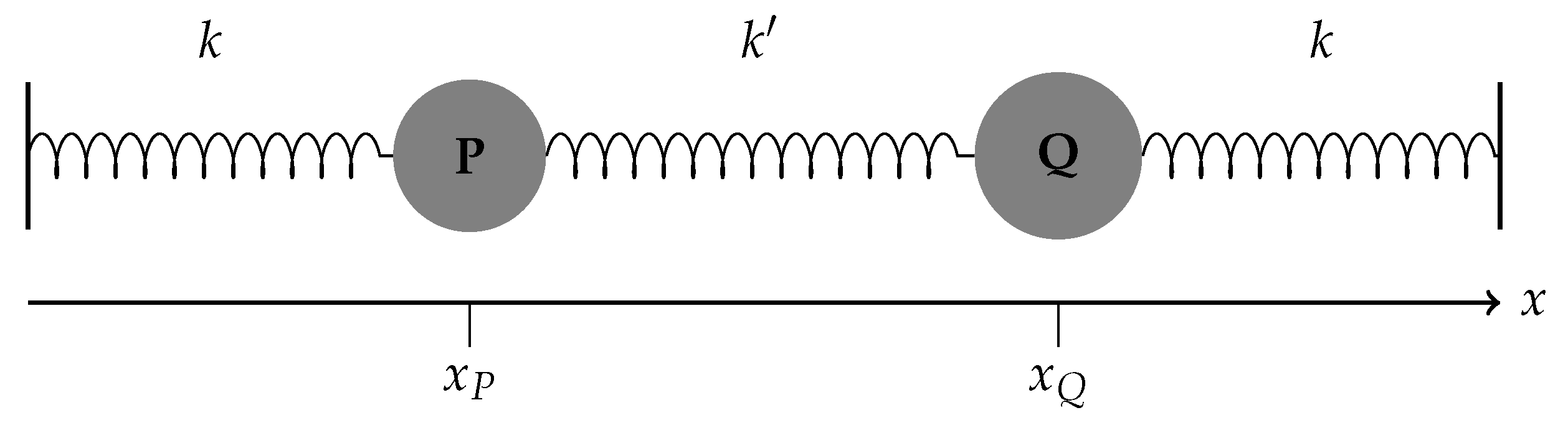
5.2. Example 2

We consider a popular model in classical mechanics called coupled oscillators (cf. [10]). Two masses P and Q are attached with springs. Assume that the masses are identical, i.e., $m_P=m_Q=m$, but the spring constants are different, as shown in the Figure 2.

Let $x_P$ be the displacement of P from its equilibrium and $x_Q$ be the displacement of Q from its equilibrium. Holding Q fixed and moving P, the force on P is

$$\begin{array}{c}\hfill F_{1P}=-k{x}_P-k^{\prime }{x}_P.\end{array}$$

Holding P fixed and moving Q, the force on P is

$$\begin{array}{c}\hfill F_{2P}=k^{\prime }{x}_Q.\end{array}$$

Thus by Newton’s second law we have

$$\begin{array}{c}\hfill m{\ddot{x}}_P=F_{1P}+F_{2P}=-(k+k^{\prime })x_P+k^{\prime }{x}_Q.\end{array}$$

Similarly, for Q we have

$$\begin{array}{c}\hfill m{\ddot{x}}_Q=-(k+k^{\prime })x_Q+k^{\prime }{x}_P.\end{array}$$

Introducing two variables $v_P={\dot{x}}_P$ and $v_Q={\dot{x}}_Q$, the above equations are equivalent to the following linear system

$$\begin{array}{c}\hfill \dot{\left(\begin{array}{c}{x}_P\\ x_Q\\ v_P\\ v_Q\end{array}\right)}=\left(\begin{array}{cccc}0& 0& 1& 0\\ 0& 0& 0& 1\\ -\frac{k+k^{\prime }}{m}& \frac{k^{\prime }}{m}& 0& 0\\ \frac{k^{\prime }}{m}& -\frac{k+k^{\prime }}{m}& 0& 0\end{array}\right)\left(\begin{array}{c}{x}_P\\ x_Q\\ v_P\\ v_Q\end{array}\right).\end{array}$$

(37)

For simplicity we denote the system by $\dot{r}\left(t\right)=Ar\left(t\right)$, where

$$\begin{array}{c}\hfill r\left(t\right)=\left(\begin{array}{c}{x}_P\left(t\right)\\ x_Q\left(t\right)\\ v_P\left(t\right)\\ v_Q\left(t\right)\end{array}\right),A=\left(\begin{array}{cccc}0& 0& 1& 0\\ 0& 0& 0& 1\\ -\frac{k+k^{\prime }}{m}& \frac{k^{\prime }}{m}& 0& 0\\ \frac{k^{\prime }}{m}& -\frac{k+k^{\prime }}{m}& 0& 0\end{array}\right).\end{array}$$

Set

$$\begin{array}{c}\hfill E=\left\{r\left(0\right)\in {\mathbb{R}}^4|\left(r_1^2\left(0\right)-r_2^2\left(0\right)\right)\left(r_3^2\left(0\right)-r_4^2\left(0\right)\right)\ne 0\right\}.\end{array}$$

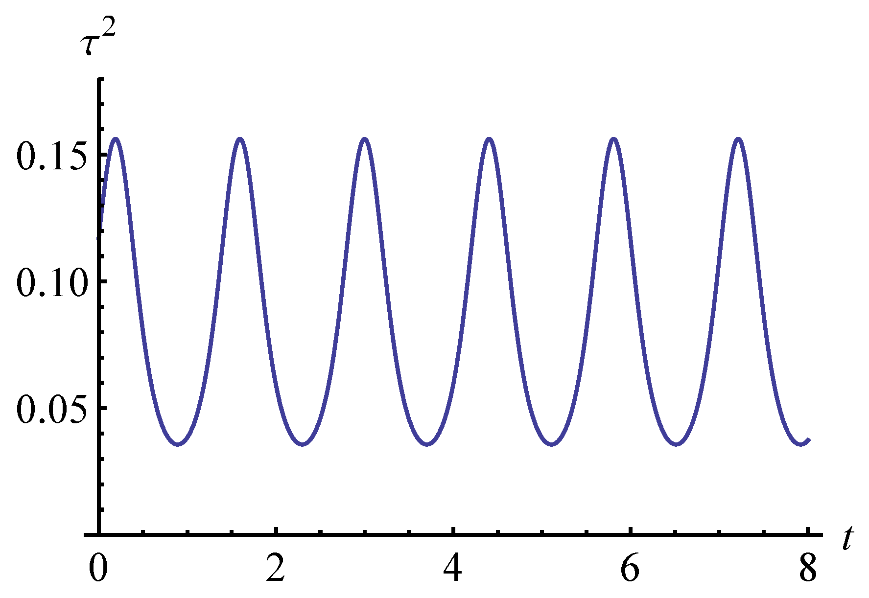
Then the Lebesgue measure of E satisfies $m\left(E\right)=+\infty .$ By direct calculation, the torsion $\tau \left(t\right)$ of the trajectory $r\left(t\right)$ is a periodic function and $\underset{t\to +\infty }{lim}\tau \left(t\right)$ does not exist for any $r\left(0\right)\in E$. Hence by Theorem 2, the zero solution of the system (37) is stable.

As an example, we suppose that $k/m=1$ and $k^{\prime }/m=2$, and the initial value $r\left(0\right)={\left(1,2,1,2\right)}^{\mathrm{T}}$. Then we have

$$\begin{array}{c}\hfill {\tau }^2\left(t\right)=\frac{\sqrt{5}sin\left(2\sqrt{5}t\right)+2cos\left(2\sqrt{5}t\right)+17}{2{\left\{\sqrt{5}sin\left(2\sqrt{5}t\right)+2cos\left(2\sqrt{5}t\right)-11\right\}}^2}.\end{array}$$

The graph of the function ${\tau }^2\left(t\right)$ is shown in Figure 3.

6. Conclusions and Future Work

The main contribution of this paper is to further develop the geometric description of stability of linear time-invariant systems in arbitrary dimension. Unlike traditional methods based on linear algebra, we focus on the curvature of curves. Specifically, the main results of this paper, Theorem 1 and Theorem 2 are proved. For the case where A is similar to a real diagonal matrix, Theorem 1 gives a relationship between the ith curvature $(i=1,2,\cdots )$ of the trajectory and the stability of the zero solution of the system $\dot{r}\left(t\right)=Ar\left(t\right)$. Further, Theorem 2 establishes a torsion discriminance for the stability of the system in the case where A is invertible.

For each theorem, we give an example to illustrate the result. In particular, we use the coupled oscillators as an example of the torsion discrimination.

In the future, we will continue to use geometric methods to describe the properties of other kinds of control systems.

References

Lyapunov, A.M. The General Problem of the Stability of Motion. Ph.D. Thesis, Univ. Kharkov, Kharkiv Oblast, Ukraine, 1892. (In Russian). [Google Scholar]
Wang, Y.; Sun, H.; Song, Y.; Cao, Y.; Zhang, S. Description of Stability for Two and Three-Dimensional Linear Time-Invariant Systems Based on Curvature and Torsion. arXiv2018, arXiv:1808.00290. [Google Scholar]
Wang, Y.; Sun, H.; Huang, S.; Song, Y. Description of Stability for Linear Time-Invariant Systems Based on the First Curvature. Math. Methods Appl. Sci.2020, 43. [Google Scholar] [CrossRef]
Gluck, H. Higher Curvatures of Curves in Euclidean Space. Am. Math. Mon.1966, 73, 699–704. [Google Scholar] [CrossRef]
Perko, L. Differential Equations and Dynamical Systems; Springer: Berlin, Germany, 1991. [Google Scholar]
Chen, C.-T. Linear System Theory and Design, 3rd ed.; Oxford University Press: Oxford, UK, 1999. [Google Scholar]
Marsden, J.E.; Ratiu, T.; Abraham, R. Manifolds, Tensor Analysis, and Applications, 3rd ed.; Springer: Berlin, Germany, 2001. [Google Scholar]
do Carmo, M.P. Differential Geometry of Curves and Surfaces; Prentice-Hall: New York, NY, USA, 1976. [Google Scholar]
Wang, Y.; Sun, H.; Cao, Y.; Zhang, S.