Algebraic Method for the Reconstruction of Partially Observed Nonlinear Systems Using Differential and Integral Embedding

Abstract

The identification of partially observed continuous nonlinear systems from noisy and incomplete data series is an actual problem in many branches of science, for example, biology, chemistry, physics, and others. Two stages are needed to reconstruct a partially observed dynamical system. First, one should reconstruct the entire phase space to restore unobserved state variables. For this purpose, the integration or differentiation of the observed data series can be performed. Then, a fast-algebraic method can be used to obtain a nonlinear system in the form of a polynomial dynamical system. In this paper, we extend the algebraic method proposed by Kera and Hasegawa to Laurent polynomials which contain negative powers of variables, unlike ordinary polynomials. We provide a theoretical basis and experimental evidence that the integration of a data series can give more accurate results than the widely used differentiation. With this technique, we reconstruct Lorenz attractor from a one-dimensional data series and B. Muthuswamy’s circuit equations from a three-dimensional data series.

1. Introduction

The problem in nonlinear dynamical system reconstruction from data series can be described as follows: For a given data series, a system must be found that produces data series that are close in a certain sense to the initial series. Obtaining system models using a limited set of observations is crucial for the reverse engineering of gene regulatory networks [1], analysis of chemical oscillations [2], studies on biological circadian rhythms [3], reconstruction of neuronal models [4], etc.

When systems described by ordinary differential equations (ODEs) are considered, one can specify the problem statement as follows: For a given data series $\left\{x_i\right\}$ and its time derivative $\left\{{\dot{x}}_i\right\}$ a system of ODEs must be reconstructed as

$$\dot{x}=f\left(x\right),$$

(1)

where $f$ is a vector function. Usually, some information about $f$ is known apriori, for instance, the possible elementary operations constituting it. These operations usually construct a group or, more specifically, a ring. One such ring is a polynomial ring which includes a set of polynomials in several variables with coefficients belonging to a certain field such as a field of real or complex numbers [5,6]. Dynamical systems with polynomial derivative functions are often referred to as polynomial dynamical systems (PDSs). In these systems, $f\left(x\right)$ is considered as

$$\dot{x}=h\otimes t\left(x\right),$$

(2)

where $h$ is the vector of unknown coefficients by the known nonlinear terms (monomials) $t$ and $\otimes$ denotes element-wise multiplication. The problem usually consists of finding all the entries in $h$, taking into account that the system can be sparse and many of these coefficients can equal zero. The set of monomials $t$ is a-priory known. Nonlinear dynamical models of Type (2) are used quite often, examples can be found in the classical works of E. Lorenz, O. Rossler, and J.C. Sprott [7]. System reconstruction in terms of PDS has been investigated since the early 1980s by many authors, for example, by J. P. Crutchfield and B. S. McNamara [8], who proposed one of the classical definitions of the problem, and J. Cremers and A. Hübler, who used Legendre polynomials as a basis for the derivative function construction [9]. Later, Taylor-like expansions were introduced by J. L. Breeden et al. [10]. Many alternatives to PDS models have been proposed, for example, neuronal networks, also including nonlinearities and coefficients found from the experimental data [11]. A neuronal network can sometimes give more precise results and is more preferable in cases of complex systems. The disadvantage of the neuronal technique is that it yields large-scale and computationally costly models. Neuronal networks and the PDS approach can also be combined, for example, for gene regulatory network identification.

The problem of finding a reliable algorithm for determining coefficients of PDS (2) is difficult, especially in case(s) of noisy and incomplete data. Determining coefficient vector $h$ can be considered as the optimization problem

$$h^{*}=\arg \min \Vert v-f\left(\mathbb{X}\right)\Vert ,$$

(3)

where $v$ is the set of observed derivatives $v=\left\{{\dot{x}}_i\right\}$, and $f\left(\mathbb{X}\right)=\{f(x_i)\}$ is a set of function values evaluated on $\left\{x_i\right\}$. The size of the unknown vector $h$ is equal to $M\times L$ where $M$ is the system dimension and $L$ is a number of available monomials.

The Problem (3) can be treated as a problem of nonlinear regression. Several researchers, for example, H. Iba and D. P. Searson et al. [12,13] developed specialized versions of genetic algorithms for solving it. The main disadvantage of genetic algorithms is that their run times are, in a general case, much longer in comparison to other approaches. Meanwhile, classical optimization methods such as Newton or quasi-Newton methods are inefficient on this problem because the optimization problem is discontinuous. When one or several coefficients become equal to zero, the nonlinear regression result changes sufficiently.

Fortunately, Problem (3) can also be considered as the linear regression problem. Indeed, consider $\Vert \cdot \Vert$ as 2-norm, and notice that since the set $\mathbb{X}$ is already known, the function values $f\left(\mathbb{X}\right)$ can be evaluated. Therefore, the least squares method (LSM) can be applied in order to obtain $h^{*}$:

$${\mathbb{E}}^{\mathrm{T}}\mathbb{E} h^{*}={\mathbb{E}}^{\mathrm{T}}v,$$

(4)

where $\mathbb{E}=f\left(\mathbb{X}\right)$.

The disadvantage of LSM is that Problem (3) is often ill-conditioned since some of the monomials vanish on the given data series and cause the singularity of the matrix ${\mathbb{E}}^{\mathrm{T}}\mathbb{E}$. To avoid this, Laubenbacher and Stigler proposed division by Gröbner basis to simplify the initial set of monomials used for regression [1], but this approach is not applicable to noisy data series.

Even if monomials do not vanish or the monomial set was somehow simplified to remove all vanishing elementary functions, the matrix ${\mathbb{E}}^{\mathrm{T}}\mathbb{E}$ usually has a large condition number which makes Problem (3) difficult to solve. Recently, D. Yogatama and N. Smith considered the application of $L_1$-regularized LSM to these types of problems, which converge better than the classical version of LSM [14]. Later, H. Kera and Y. Hasegawa proposed excluding vanishing polynomials using the approximate Buhberger-Müller algorithm and, then, deleting minor terms from regression using a specialized procedure [15]. The latter algorithm, further referred to as the Kera-Hasegawa (KH) method, underlies the reconstruction procedure developed in this paper.

From a physical point of view, some state variables needed to perform the reconstruction procedure can be unknown. The simplest case is when only system states are known and the derivatives are not, so numerical differentiation should be applied. Howeve, if the system is partially observed, phase space reconstruction must be performed. For example, when a circuit with a memristive element is considered, one of its state variables, magnetic flux or charge in a memristive device, cannot be directly measured in a macroscopic scale [16]. The problem is more complicated in the domain of physical chemistry where only one variable is usually observed, for example, in Belousov-Zhabotinsky reaction this is Br-ISE electric potential [17]. Using the well-known Takens’ embedding theorem [17] we can reconstruct the discrete-time system phase space using a shifted time series. For continuous-time reconstruction, we can use differentiation or integration. The latter technique is used quite rarely because it can cause the emergence of linear trends in integrated data but we will show how to avoid this and why it is more preferable than differentiation.

The main aim of this paper is to establish an efficient and reliable technique for identifying chaotic circuits, especially, ones with nonlinear elements with unknown parameters. The problem arises from the fact that real circuits even with simple nonlinearities and known parameters need certain parameter optimization for simulation despite the theoretical prediction that the circuit can accurately correspond to the ODE [18]. When the circuit contains a nonlinear element, the problem becomes more complicated since the relevant model of this element may also be different from the prediction. For example, it has recently been shown that original HP models are irrelevant to the actual resistance switching devices with memory effect [16]. The relevant model proposed in this work [16] contains exponents, hyperbolic trigonometric functions and negative powers.

This paper is organized as follows: First, we describe how PDS can be reconstructed from complete data using the extended Kera-Hasegawa method; second, we explain how these results can be applied to data series lacking some state variables; third, we carry out computational experiments showing the validity of the approach, to be more precise, we reconstruct the Lorenz system from 1-dimensional data series and a 4-dimensional memristive circuit proposed by B. Muthuswamy [19] using incomplete 3-dimensional data and we show that the accuracy of numerical integration and differentiation plays an important role in the success of reconstruction, even though the reconstruction method is noise-tolerant; finally, we discuss the limitations of the proposed approach and give a conclusion.

2. Algebraic Method for ODE Reconstruction

In this section, we describe an algebraic approach to the system reconstruction method based on subsequent application of the approximate Buchberger–Möller method, the least-squares method and deleting minor terms method, close to the method proposed by Kera and Hasegawa, but we extend this approach to the Laurent polynomials which can have negative powers of monomials in comparison with ordinary polynomials with nonnegative powers only.

2.1. Polynomial Rings, Ideals, ABM Algorithm

Consider a nonlinear function in Equation (1) as

$$f\left(x\right)=\left(\begin{array}{c} {\displaystyle {\displaystyle \sum }_{i=1}^L}{h}_{1i}{t}_i\left(x\right)\\ ⋮\\ {\displaystyle {\displaystyle \sum }_{i=1}^L}{h}_{Mi}{t}_i\left(x\right)\end{array}\right),$$

(5)

where $M$ is dimension,$L$ is the number of elementary monomials $t_i$, and $h_{ji}$ are the coefficients of each elementary monomial, and $x={\left(x_1, x_2, \dots x_M\right)}^{\mathrm{T}}$. Each component of Equation (5) represented in the form ${\displaystyle \sum }_{i=1}^L{h}_{1i}{t}_i\left(x\right)$ is a polynomial. The monomials have general form as

$$t_i\left(x\right)={\displaystyle \prod }_{i=j}^{M}x{ }_j^{{\alpha }_{ij}}$$

(6)

where ${\alpha }_{ij}$ are the powers of each variable. The polynomial functions

$$f_k\left(x\right)={\displaystyle \sum }_{i=1}^L{h}_{ki}{t}_i\left(x\right)$$

(7)

form a polynomial ring $\mathbb{P}$ over the field $\mathbb{F}$, where operations of addition and multiplication are defined as usual. More precisely, $\mathbb{P}$ is an Abelian group under addition since it is associative, commutative, has an additive inverse and has zero element $f\left(x\right)=0$, $\mathbb{P}$ is monoid under multiplication since it is associative and has an identity element $f\left(x\right)=1$ which is exactly

$$f\left(x\right)=1\cdot {\displaystyle \prod }_{i=j}^{M}x{ }_j^0,$$

also this multiplication is distributive. The field over which the ring is defined determines the properties of the coefficients $h_{ki}\in \mathbb{F}$. In this paper, we consider $\mathbb{P}$ over a field of real numbers $ℝ$.

When ${\alpha }_{ij}\in \mathbb{N}$, the functions of Equation (6) form ordinary polynomials, or Taylor-like expressions, e.g., for the two-variable function it can be

$$f\left(x,y\right)=h_{11}+h_{12}x+h_{13}y+h_{14}{x}^2+h_{15}xy+h_{16}{y}^2+\cdots$$

(8)

When ${\alpha }_{ij}\in \mathbb{Z}$, the functions for Equation (5) are called Laurent polynomials where powers are conventionally defined within a symmetric interval ${\alpha }_{ij}\in {\left[-M,M\right]}_{\mathbb{Z}}$, but we will not require this property further. The terms in Equation (8) can be ordered in various ways. We will consider a degree-lexicographic order, where we primarily consider the power of the entire monomial defined as

$${\alpha }_i={\displaystyle \sum }_{j=1}^M{\alpha }_{ij}.$$

Second, we consider the powers of variables selected alphabetically organized in ascending order of absolute value of power. This may be exemplified for a set of Laurent monomials of 2 variables and order in $\left[-1;1\right]$ as

$$\mathbb{T}\left(x,y\right)= \left\{x^{-1}, y^{-1},1,x{y}^{-1},x^{-1}y, x,y\right\}.$$

Originally, only positive powers are considered in degree-lexicographic order, so we introduce this equation here by analogy; for discussion, see Section 4.

The order ideal $O$ of the polynomial ring $\mathbb{P}$ is a finite set of monomials in $\mathbb{T}$ if it is closed under divisors, i.e., satisfying the condition: for each monomial $t\in O$ all monomials $t_j$ dividing it also belong to $O$. A “border” of the order ideal $\partial O$ in an ordinary polynomial ring is a set of monomials in $\mathbb{T}$ defined as

$$\partial O=\left(x_{1}O\cup x_{2}O\cup \dots \cup x_{M}O\right)-O,$$

(9)

where “minus” denotes set subtraction. If the monomial set $O=\left\{1,x,y\right\}$ is an order ideal in an ordinary polynomial ring, its border is

$$\partial O=\left\{x^2,xy,y^2\right\}.$$

In Laurent polynomial ring, a border is defined similarly to Equation (9) but also includes negative powers $x_i^{-1},i=1\dots M$:

$$\partial O=\left(x_{1}O\cup x_{2}O\cup \dots \cup x_{M}O\cup x_1^{-1}O{x}_2^{-1}O\cup \dots \cup x_M^{-1}O\right)-O.$$

The vanishing ideal of a set of data points $\mathbb{X}$ is a set of all polynomials vanishing (i.e., equals to zero) on $\mathbb{X}$:

$$\mathbb{I}\left(\mathbb{X}\right)=\{p\in \mathbb{P} |p\left(x\right)=0, \forall x\in \mathbb{X}\}.$$

(10)

The vanishing ideal $\mathbb{I}\left(\mathbb{X}\right)$ can be spanned by a finite set of polynomials called the basis of $\mathbb{I}\left(\mathbb{X}\right)$. Let $O=\left\{t_1\dots t_L\right\}$ be an order ideal with a border $\partial O=\left\{b_1\dots b_{\nu }\right\}$. Let $G=\left\{g_1\dots g_{\nu }\right\}\subset \mathbb{P}$ be a set of polynomials, and there is an ideal $\mathbb{I}\subseteq \mathbb{P}$. The set $G$ is an $O$-border prebasis if the polynomials in it have the form

$$g_j=b_j-{\displaystyle \sum }_{i=1}^L{\alpha }_{ij} t_i \mathrm{for} j\in \left[1\dots \nu \right], {\alpha }_{ij}\in \mathbb{F}.$$

(11)

The set $G$ is an $O$-border basis of $\mathbb{I}$ if $G$ generates $\mathbb{I}$ and if the residue classes of the terms in $O$ constitute a vector basis of $\mathbb{P}-\mathbb{I}$. Several other bases are known, such as Gröbner basis and Macaulay basis. To find a border basis, Buchberger–Möller (BM) algorithms can be used [15]. Border basis $G$ is called approximate if $\Vert g{\left(\mathbb{X}\right)\Vert }_2<ϵ$, where $g\in G$ and $ϵ$ is a small positive number. Modification of BM algorithm, known as the approximate Buchberger–Möller (ABM) algorithm can be used to compute an approximate border basis on a noisy dataset $\mathbb{X}$.

We also define the evaluation map $ℰ$, which transforms a given dataset $\mathbb{X}=\left\{x_1\dots x_N\right\}$ into a matrix ${ℰ}_{\mathbb{T}}\left(\mathbb{X}\right)={\mathbb{E}}_{\mathbb{T}}$, where

$${\mathbb{E}}_{\mathbb{T}}=\left(\begin{array}{ccc}{t}_1\left(x_1\right)& \dots & t_L\left(x_1\right)\\ ⋮& \ddots & ⋮\\ t_1\left(x_N\right)& \dots & t_L\left(x_N\right)\end{array}\right).$$

The ABM algorithm can be described as follows. Suppose, we have a dataset $\mathbb{X}$, a tolerance $ϵ$, and set of monomials $\sigma \subset \mathbb{T}$ in degree-lexicographic order. We should obtain a border basis $G$ and an order ideal $O$. We start with degree $d=1$ and $O=\left\{1\right\}$. Let $L\subset \sigma$initially contain all terms of degree 1. Then, the process starts while the order $d$ is not greater than the maximal order defined as $\max \mathrm{deg}\sigma$ and $L$ is not empty. At the current step, all monomials of degree $d-1$ have been already processed. We estimate the vector $A$ on the next monomial in $\sigma$ as

$$A={ℰ}_t\left(\mathbb{X}\right),t\in L,$$

(12)

and, then, remove it from $L$. Let ${\mathsf{\lambda }}_{\min }$ be the smallest eigenvalue of the matrix $A^{T}A$

$${\mathsf{\lambda }}_{\min }={\mathsf{\lambda }}_i,i=\arg \min \left|\mathrm{eig} \left(A^{T}A\right)\right|,$$

and if it satisfies the condition

$$\sqrt{{\mathsf{\lambda }}_{\min }}>ϵ,$$

then $t$ is appended to $O$ and all the polynomials of order $d+1$ are added to $\partial O$. A polynomial with coefficients defined by an eigenvector of $A^{T}A$ corresponding to ${\mathsf{\lambda }}_{\min }$ is added to $G$.

Application of ABM algorithm to the dataset $\mathbb{X}$ and the set of initial monomials $\sigma$ allows obtaining $O$ and ensures that any polynomial

$$p\left(x\right)={\displaystyle \sum }_{i=1}^L{h}_{ki}{o}_i\left(x_k\right),$$

where $o_i\in O$, does not vanish on $\mathbb{X}$, even though $O$ can be, strictly speaking, not always an order ideal [15].

2.2. KH Algorithm for Polynomial Function Reconstruction

Consider a dataset $\mathbb{X}=\left\{x_1,\dots ,x_M\right\}$ which can be represented as observation vectors $x_i$ for i-th state variable, M is the system dimension. Each data vector has N observation points. Using the order ideal $O$ as a set of basis monomials, one can evaluate them on a given dataset $\mathbb{X}$ and then build an interpolation, using derivatives set $\mathbb{V}=\left\{v_1,\dots ,v_M\right\}$ which is also given or can be derived from $\mathbb{X}$ by the relation $v_i=\dot{x_i}$:

$$v_k={\displaystyle \sum }_{i=1}^L{h}_{ki}{o}_i\left(x_k\right).$$

(13)

In each dimension, Equation (13) can be reconstructed using the least squares method. Denote $\mathbb{E}={ℰ}_O\left(\mathbb{X}\right)$ and transform Equation (13) into a linear equation:

$$v_k=\mathbb{E}{h}_k.$$

(14)

Equation (14) is usually considered as overdetermined, since the number of estimated points can be arbitrary and, in the presence of noise, a large number of observations are a necessary condition for obtaining a reliable solution. The overdetermined Equation (14) can be solved using the ordinary least squares method, obtaining the minimum

$$h^{*}=\arg \min {\Vert v_k-\mathbb{E}{h}_k\Vert }^2$$

(15)

by analytical Formula (4). Due to the presence of noise and since it is supposed that the vector $h_k$ is sparse, $L_1$-regularization is recommended to obtain better results:

$$h^{*}=\arg \min \left(\frac{1}{2}{\Vert v_k-\mathbb{E}{h}_k\Vert }^2-\mathsf{\lambda }\left|h_k\right|\right),$$

(16)

where $\mathsf{\lambda }$ is a regularization parameter. Increasing $\mathsf{\lambda }$ provides a sparser solution. Problem (16) is also known as a basis pursuit denoising (BPDN) problem, and several special optimization methods have been proposed for solving it, e.g., Nesterov method [20,21]. If it is assumed that $h^{*}$ is dense, $L_2$-regularization or Tikhonov regularization [22] can be applied:

$$h^{*}=\arg \min \left(\frac{1}{2}{\Vert v_k-\mathbb{E}{h}_k\Vert }^2-\mathsf{\lambda }{\Vert h_k\Vert }^2\right),$$

(17)

with a known solution in terms of matrices:

$$h^{*}={\left({\mathbb{E}}^{\mathrm{T}}\mathbb{E}+\mathsf{\lambda }NI\right)}^{-1}({\mathbb{E}}^{\mathrm{T}}v),$$

(18)

where $I$ is an identity matrix [23].

Kera and Hasegawa [15] proposed removing minor terms from the interpolation polynomial

$$H_k\left(x\right)={\displaystyle \sum }_{i=1}^L{h}_{ki}{o}_i\left(x\right)$$

(19)

using a special procedure based on an estimation

$$w_i=\Vert {ℰ}_{O_i}\left(\mathbb{X}\right)h_{ik}\Vert .$$

For each term in a polynomial $h_{ki}{o}_i\left(x\right)$ its weight (20) is estimated, and terms with minimal weight are subsequently removed from the interpolation while the error of approximation remains within a given tolerance $\eta$:

$$\frac{1}{N}\Vert v_k-H_k\left(\mathbb{X}\right)\Vert \le \eta .$$

(20)

Following Kera and Hasegawa, we call this procedure delMinorTerms. It ensures that the solution is sparse enough even if the data is contaminated with noise.

The Kera–Hasegawa (KH) PDS reconstruction method finds a set of interpolating polynomials $ℍ$ in $\mathbb{P}=\left(\mathbb{T}\times ℝ\right)$ of type (19), where $\times$ is the Cartesian multiplication, satisfying $\left(ℍ\subset \mathbb{P}: H_k\left(\mathbb{X}\right)\approx v_k\right)$ for a given $\mathbb{X}$ and $\mathbb{V}$. Firstly, it performs the ABM algorithm to remove monomials from $\mathbb{T}$ vanishing on $\mathbb{X}$, comprising an order ideal $O$ of $\mathbb{T}$. Next, it applies $L_1$-regularizated LSM to find an interpolation polynomial on $O\times ℝ$ and then runs delMinorTerms to ensure that the interpolated polynomials are sparse while the accuracy criterion Equation (20) is satisfied.

2.3. Phase Space Reconstruction Using Integration Embedding

The KH method can be performed only if $\mathbb{X}$ and $\mathbb{V}$ are complete, i.e., the dimension M of the reconstructed system corresponds to dimensions of $\mathbb{X}$ and $\mathbb{V}$. In the general case, we can observe only one or several state variables, and thus we need to reconstruct the entire phase space. The well-known F. Takens’ theorem [23] states that having a time-delayed series of a single-variable signal $\left\{x\left[n\right],x\left[n-1\right],x\left[n-2\right],\dots ,x\left[n-\left(M-1\right)\right]\right\}$, we can reconstruct M-dimensional phase space due to time delay embedding, and, similarly, N. Packard et al. [24] proposed reconstructing M-dimensional phase using $M-1$ subsequent derivatives

$$\left\{x\left[n\right],\frac{dx\left[n\right]}{dt},\dots ,\frac{d^{M-1}x\left[n\right]}{d{t}^{M-1}}\right\},$$

(21)

due to differential embedding. Recently, J. Lekscha and R. Donner [25] have shown that reconstruction is possible in the case of non-uniformly sampled and noisy time series as well, which is an important result for practical use.

Unlike the differential embedding approach, integral embedding did not become popular in scientific literature, despite being more useful in several practical cases.

Lemma 1.

M-dimensional phase space can be reconstructed due to integral embedding, and a trajectory $ℱ$of the system$F$reconstructed from time series$x\left[n\right]$can be written as:

$$\left\{\underset{M-1}{\underbrace{\int \dots \int }}x\left[n\right]d{t}^{M-1}+C_{M-1}\left(t\right),\dots ,\int x\left[n\right]dt+C_1,x\left[n\right]\right\},$$

(22)

where$C_{M-1}\left(t\right)$is a residual polynomial whose general form is:

$$C_K\left(t\right)=C_K+C_{K-1}t+C_{K-2}{t}^2+\dots +C_1{t}^{K-1},$$

(23)

where$K$is a natural number.

Proof. 

A system of ODEs in the Cauchy normal form is usually organized so as

$$\frac{d}{dt}{x}_j=x_{j+1},$$

where the state variable $x_j$ is related to the variable of the next index through differentiation. It can also be written through the integration

$$x_j=\int x_{j+1}dt+C_j, j\in \left[1,M-1\right],$$

(24)

where $C_j$ is a constant depending on the initial condition. Equation (24) can be used for subsequent integration of state variables for reconstructing the trajectory in a full phase space when variables $x_1\dots x_{j-1}$ are known. After K integrations of a time series given by $x_1$, we obtain

$$x_K=\underset{K}{\underbrace{\int \dots \int }}{x}_1\mathrm{dt}+C_K+C_{K-1}t+C_{K-2}{t}^2+\dots +C_1{t}^{K-1},$$

from which Equations (22) and (23) follow obviously. □

Corollary 1.

Since the polynomial residual Equation (23) grows very fast if$t^{K-1}$is large enough, it is undesirable if we consider a computer implementation of the reconstruction algorithm. Otherwise, the accuracy of the data representation may suffer. We propose the following procedure for obtaining$x_j$. First, we choose zero initial condition to detect and integrate$x_{j+1}$on a given time interval$\left[t_0,t_1\right]$:

$$x_j^{*}={{\displaystyle \int }}_{t_0}^{t_1}{x}_{j+1}dt.$$

Then, we estimate its mean value$\langle x_j\rangle$, and supposing$C_j=$$\langle x_j\rangle$, subtract it obtaining the desired solution$x_j=x_j^{*}-C_j.$Another way is to de-trend the second integral containing$C_{j}t$with a specialized procedure, e.g., detrend function in a MATLAB environment.

The system reconstructed using integration embedding is equivalent to the system reconstructed using differential embedding up to $M-1$ differentiations. More strictly, this can be formulated as Lemma 2.

Lemma 2.

Suppose, there is a map$G\left(t,y\right):ℝ\times {ℝ}^M\to {ℝ}^M$,$t\in ℝ, y\in {ℝ}^M$which projects$\mathcal{G}$onto the phase space${ℝ}^M$, can be obtained via subsequent differentiation of the one-dimensional trajectory${\mathcal{G}}_1$corresponding to the state variable$y_1$. Then, then a dynamical system$\left(t,x\right):ℝ\times {ℝ}^M\to {ℝ}^M$,$x\in {ℝ}^M$exists which projects$ℱ$onto the phase space${ℝ}^M$can be obtained via subsequent integration of the one-dimensional trajectory${ℱ}_M=G_1$corresponding to the state variable$x_M$.

Proof. 

The following ODE describes a dynamical system $G\left(t,y\right)$ due to the condition that subsequent differentiation of one-dimensional trajectory $y_1$ generates $\mathcal{G}$

$$\{\begin{array}{c}\frac{d}{dt}{y}_1=y_2,\hfill \\ \hfill ⋮\hfill \\ \frac{d}{dt}{y}_{M-1}=y_M,\hfill \\ \frac{d}{dt}{y}_M=g\left(t,y\right).\hfill \end{array}$$

(25)

Since ${\mathcal{G}}_1={ℱ}_M$ the corresponding state variables are equal: $y_1=x_M$. The condition that the projection $ℱ$ of the map $F$ onto the entire phase space can be obtained via subsequent integration of its one-dimensional component ${ℱ}_M$ can be expressed in the form of Equation (24). Consequently, the following ODE describes $F\left(t,x\right)$:

$$\{\begin{array}{c}\frac{d}{dt}{x}_1=x_2,\hfill \\ \hfill ⋮\hfill \\ \frac{d}{dt}{x}_{M-1}=x_M,\hfill \\ \frac{d}{dt}{x}_M=f\left(t,x\right),\hfill \end{array}$$

where $f\left(t,x\right)$ is a differentiable function. It is related with $y_1$ in the following way: $y_1= \int f\left(t,x\right)dt+C$. □

Corollary 2.

A dynamical system$F$which can be reconstructed via integration embedding exists if the system$G$which can be reconstructed via differential embedding exists.

The ODE representation of a partially observed system with K observed variables and M-dimensional entirely phase space can be represented in the following way:

$$\{\begin{array}{c}\begin{array}{c}\frac{d}{dt}{x}_1=g_1\left(x\right),\\ ⋮\end{array}\\ \frac{d}{dt}{x}_K=g_K\left(x\right),\\ \begin{array}{c}\frac{d}{dt}{x}_{K+1}=x_K,\\ ⋮\\ \frac{d}{dt}{x}_M=x_{M-1},\end{array}\end{array}$$

(26)

where $f_j\left(x\right)$ is a scalar function. Missing derivatives of orders $\left\{K+1,\dots ,M\right\}$ can be found numerically. Finite-difference-based numerical differentiation is the most common approach, but some other techniques can be used as well, e.g., numerical differentiation based on Legendre polynomials [25]. If the known state variables are denoted $x_{K+1}, \dots , x_M$, the system reconstructed via integration reads

$$\{\begin{array}{c}\begin{array}{c}\frac{d}{dt}{x}_1=x_2,\\ \hfill ⋮\end{array}\hfill \\ \frac{d}{dt}{x}_K=x_{K+1},\hfill \\ \begin{array}{c}\frac{d}{dt}{x}_{K+1}=f_{K+1}\left(x\right),\hfill \\ ⋮\\ \frac{d}{dt}{x}_M=f_M\left(x\right),\hfill \end{array}\hfill \end{array}$$

(27)

which is an alternative form of Equation (26) with other variables. □

The number of dimensions $M$ can be selected concerning its physical sense or with one of the several algorithms, e.g., false nearest neighbor (FNN) algorithm [26,27], or estimating one of the fractal dimensions or entropies [28].

The embedded integration approach is more useful in some practical cases due to the following two theorems. Theorem 1 considers a case appearing in many practical applications when the differential embedding approach cannot give a valid reconstruction due to the non-uniqueness of the solution corresponding to the reconstructed trajectory $ℱ$.

Theorem 1.

A function$f$(t) determined on$ℝ$exists, satisfying the following conditions:

(1) 

$f$(t) is a function that produces time series u =$\left\{f\left(t_i\right)\right\}$being a one-dimensional projection of a M-dimensional trajectory$ℱ$of the dynamical system$F$;

(2) 

$f$(t) is continuous and satisfies the Lipchitz condition

$$\left|f\left(t_1\right)-f\left(t_2\right)\right|\le K\left|t_1-t_2\right|$$

where$K>0$is the Lipchitz constant;

(3) 

an M-dimensional trajectory$\widehat{ℱ}$can be reconstructed from time series u using differentiation which does not satisfy the condition of the uniqueness of the solution;

(4) 

an M-dimensional trajectory$\widetilde{ℱ}$can be reconstructed from time series u using integration that satisfies the condition of uniqueness of the solution and thus is topologically valid.

Proof. 

Consider a continuous function that satisfies the following conditions. First, there exists an infinite set of time points at which the function $f$ and its derivatives equal an arbitrary number $a\in ℝ$:

$$\exists \mathit{\tau }: f\left(t_0\right)=a,f^{\prime }\left(t_0\right)=a,\dots ,f^{M-1}\left(t_0\right)=a,t_0\in \mathsf{\tau }.$$

(28)

At other time points the function $f$ differs from $a$:

$$f\left(t_j\right)\ne a, f^{\prime }\left(t_j\right)\ne a,\dots , f^{M-1}\left(t_j\right)\ne a, t_0\notin \mathsf{\tau }.$$

(29)

Second, for a sufficiently large number $Q\in \mathbb{N}$: $M\le Q$ there exist two time points $t_i$ and $t_j$, where the function changes its value relatively to $a$:

$$f\exists \left(t_j,t_i\right):f^{\left(q\right)}\left(t_i\right)\langle a;f^{\left(q\right)}\left(t_j\right)\rangle a,$$

(30)

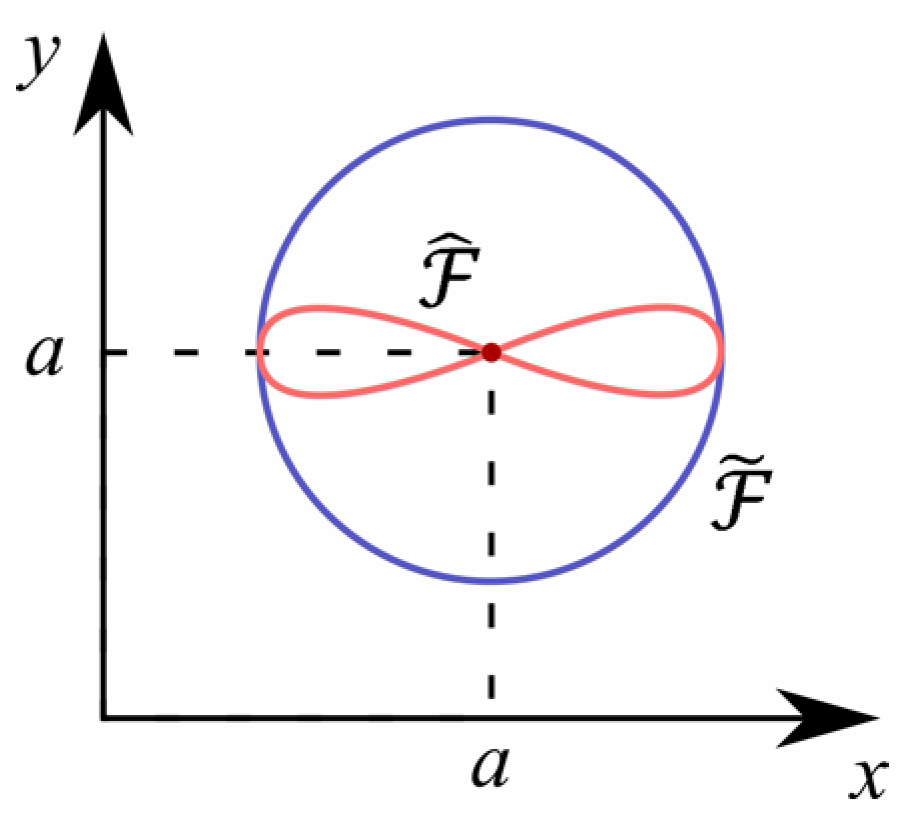
$q\in \left[0;Q\right]$. Then, under this conditions, reconstruction by differentiation yields in a phase space where the point $x_a={\left(a,a,\dots ,a\right)}^{\mathrm{T}}$ is a point at which at least two trajectory loops are connected and therefore the uniqueness of the solution is violated: starting from this point and having no apriori information of which branch can be selected we can neither predict the next state of the system nor determine the previous state of the system. Therefore, the trajectory $\widehat{ℱ}$ reconstructed from time series u using differentiation does not satisfy the condition of uniqueness of the solution. Meanwhile, due to Lemma 1 and Lemma 2, it is possible to obtain M-dimensional trajectory $\widetilde{ℱ}$ from time series u using integration. Due to Corollary 1 it is possible to select such integration constants $C_j$ when $u$ and its integrals are not equal to $a$ so it may satisfy the condition of the uniqueness of the solution and thus $\widetilde{ℱ}$ is topologically valid. Figure 1 illustrates the phase space geometry. □

Time series u = $\left\{f\left(t_i\right)\right\}$ satisfying conditions 2–4 of the Theorem 1 when $a=0$are rather common in biology, medicine, genetics and neuroscience.

Theorem 2 is dedicated to noise-amplifying properties of differentiation operators. In the presence of additive white Gaussian noise, when the sampling frequency is high enough and the spectral density of the signal is mostly low-frequency, differentiation tends to decrease the signal-to-noise ratio (SNR), while integration does not.

Theorem 2.

Denote the Fourier transform of a signal$u\left(t\right)$as$U\left(\omega \right)$. Let the power spectrum of$u$lie almost entirely in a frequency interval$\left[{\omega }_0, {\omega }_1\right]$. Let$\xi \left(t\right)$be the additive white Gaussian noise (AWGN) contaminating$u$. Then:

(1) 

after differentiation, the SNR of$\frac{d}{dt}u$will be smaller than the SNR of$u$;

(2) 

after integration, the SNR of$\int udt$will be at least not smaller than the SNR of$u$.

Proof. 

Recall, the signal-to-noise ratio is determined as

$$\mathrm{SNR}=\frac{A_u^2}{A_{\xi }^2 },$$

where $A_u$ is root-mean-square (RMS) amplitude of the signal with its square equal to

$$A_u^2=\underset{\mathrm{T}\to \infty }{\lim }{{\displaystyle \int }}_0^T\frac{{\left[u\left(t\right)\right]}^2}{T}dt,$$

where $T$ is time interval, and $A_{\xi }$ is RMS amplitude of the noise.

Denote the sampling frequency as ${\omega }_s$. Denote the Fourier transform of the noise $\xi \left(t\right)$ as $\mathsf{\Xi }\left(\omega \right)$. Then, the power spectral density of the noise calculated within frequency interval $\omega \in [0;{\omega }_s$/2] is

$$S_{\xi \xi }\left(\omega \right)=\underset{T\to \infty }{\lim }\frac{ {\left|\mathsf{\Xi }\left(\omega \right)\right|}^2}{T}$$

According to Parseval’s theorem,

$${{\displaystyle \int }}_0^T{\left[\xi \left(t\right)\right]}^{2}dt={{\displaystyle \int }}_0^{\frac{{\omega }_s}{2}}|\mathsf{\Xi }\left(\omega \right){|}^{2}dt,$$

and the same is true for the signal. Consequently, from Equation (31) and Equations in (32) SNR may be expressed through power spectra as

$$\mathrm{SNR} = \underset{T\to \infty }{\lim }\frac{{{\displaystyle \int }}_0^{\frac{{\omega }_s}{2}}{S}_{uu}\left(\omega \right)d\omega }{{{\displaystyle \int }}_0^{\frac{{\omega }_s}{2}}{S}_{\xi \xi }\left(\omega \right)d\omega }$$

Note that AWGN has a uniform power spectral density, i.e.,

$$\forall \omega \in \left[0;\frac{{\omega }_s}{2}\right]:S_{\xi \xi }\left(\omega \right)=\langle S_{\xi \xi }\rangle .$$

The condition that the power spectrum of $u$ lie almost entirely in a frequency interval $\left[{\omega }_0, {\omega }_1\right]$ means that its power spectrum $S_{uu}\left(\omega \right)$ satisfies the condition:

$${{\displaystyle \int }}_0^{{\omega }_1}{S}_{uu}\left(\omega \right)d\omega >q{{\displaystyle \int }}_0^{{\omega }_s/2}{S}_{uu}\left(\omega \right)d\omega ,$$

where $0<q<1$ is a positive real number close to 1, and ${\omega }_1$ is a frequency up to which almost the whole spectrum is contained, usually, ${\omega }_1<\frac{{\omega }_s}{2\dots 10}$. The gap between ${\omega }_1$ and ${\omega }_s/2$ is almost occupied by the noise only, see Figure 2a. Consequently, in this case, a formula for SNR can be rewritten as:

$$\mathrm{SNR} = \underset{T\to \infty }{\lim }\frac{{{\displaystyle \int }}_0^{{\omega }_1}{S}_{uu}\left(\omega \right)d\omega }{{{\displaystyle \int }}_0^{\frac{{\omega }_s}{2}}{S}_{\xi \xi }\left(\omega \right)d\omega }$$

(31)

Consider integration and differentiation acting at $u$. Taking Fourier transform, obtain

$$\{\begin{array}{c}{{\displaystyle \int }}_0^{T}u\left(t\right)dt\doteqdot \frac{1}{j\omega }U\left(\omega \right)\\ \frac{d}{dt}u\left(t\right)\doteqdot j\omega U\left(\omega \right)\end{array},$$

where $j$ is the imaginary unit. The same is true for the noise. Denote $\frac{d}{dt}u\left(t\right)=\dot{u}\left(t\right)$, ${{\displaystyle \int }}_0^{T}u\left(t\right)dt=\mathcal{U}\left(t\right)$, $\frac{d}{dt}\xi \left(t\right)=\dot{\xi }\left(t\right)$, $\frac{d}{dt}\xi \left(t\right)=\mathsf{\Xi }\left(t\right)$. Then, corresponding spectral densities are:

$$\{\begin{array}{c}{S}_{\dot{u}\dot{u}}\left(\omega \right)={\omega }^2{S}_{uu}\left(\omega \right),\\ S_{\mathcal{U}\mathcal{U}}\left(\omega \right)=\frac{1}{{\omega }^2}{S}_{uu}\left(\omega \right),\\ S_{\dot{\xi }\dot{\xi } }\left(\omega \right)={\omega }^2{S}_{\xi \xi }\left(\omega \right),\\ S_{\mathsf{\Xi }\mathsf{\Xi }}\left(\omega \right)=\frac{1}{{\omega }^2}{S}_{\mathsf{\Xi }\mathsf{\Xi }}\left(\omega \right).\end{array}$$

(32)

From Equation (31) and Equations in (32), SNR of the differentiated signal is:

$${\mathrm{SNR}}_{\mathrm{D}} = \underset{T\to \infty }{\lim }\frac{{{\displaystyle \int }}_0^{{\omega }_1}{\omega }^2{S}_{uu}\left(\omega \right)d\omega }{{{\displaystyle \int }}_0^{\frac{{\omega }_s}{2}}{\omega }^2{S}_{\xi \xi }\left(\omega \right)d\omega }=\underset{T\to \infty }{\lim }\frac{{{\displaystyle \int }}_0^{{\omega }_1}{\omega }^2{S}_{uu}\left(\omega \right)d\omega }{\frac{{\omega }_s{}^3}{24}\langle S_{\xi \xi }\rangle }.$$

Due to Hölder’s inequality, and the fact that both ${\omega }^2$ and $S_{uu}\left(\omega \right)$ are nonnegative,

$${\mathrm{SNR}}_{\mathrm{D}}\le \underset{T\to \infty }{\lim }\frac{\frac{{\omega }_1^3}{3}{{\displaystyle \int }}_0^{{\omega }_1}{S}_{uu}\left(\omega \right)d\omega }{\frac{{\omega }_s{}^3}{24}\langle S_{\xi \xi }\rangle }={\left(\frac{2{\omega }_1}{{\omega }_s}\right)}^3\mathrm{SNR}.$$

Since $\frac{2{\omega }_1}{{\omega }_s}<1$, the ${\mathrm{SNR}}_{\mathrm{D}}$ is never greater than the SNR of the original signal under the above made assumptions.

For the integration operator, from Equation (31) and Equations in (32),

$${\mathrm{SNR}}_{\mathrm{I}} = \underset{T\to \infty }{\lim }\frac{{{\displaystyle \int }}_0^{{\omega }_1}\frac{1}{{\omega }^2}{S}_{uu}\left(\omega \right)d\omega }{{{\displaystyle \int }}_0^{\frac{{\omega }_s}{2}}\frac{1}{{\omega }^2}{S}_{\xi \xi }\left(\omega \right)d\omega }=\underset{T\to \infty }{\lim }\frac{{{\displaystyle \int }}_0^{{\omega }_1}\frac{1}{{\omega }^2}{S}_{uu}\left(\omega \right)d\omega }{-\frac{2}{{\omega }_s}\langle S_{\xi \xi }\rangle }.$$

Again, due to Hölder’s inequality,

$${\mathrm{SNR}}_{\mathrm{I}}\le \underset{T\to \infty }{\lim }\frac{\frac{1}{{\omega }_1}{{\displaystyle \int }}_0^{{\omega }_1}{S}_{uu}\left(\omega \right)d\omega }{\frac{2}{{\omega }_s}\langle S_{\xi \xi }\rangle }=\frac{{\omega }_s}{2{\omega }_1}\mathrm{SNR}.$$

Therefore, while the ${\mathrm{SNR}}_{\mathrm{I}}$ is not obligatorily greater than the SNR of the original signal, it is not necessarily less than it in contrast to the case of using differentiation. □

Theorem 2 is in good correspondence with the signal processing theory [29] from which it is known that differentiation operator relates to a high-pass filter, and amplifies high-frequency noise, while integration operator relates to a low-pass filter.

2.4. Description of the Proposed Reconstruction Technique

The overall proposed technique is described as follows:

First, we consider the time series set $\mathbb{U}$ of a partially observed dynamical system and its derivative $\mathbb{W}$. Using both integral or differential embedding, preferring the first one due to Theorems 1 and 2, we reconstruct the phase space and the $M$-dimensional phase space trajectory $\mathbb{X}$. In this paper we suppose that $M$ is already known. If not, the FNN algorithm or other dimension-finding algorithms can be applied. For the reasons why we do not reject differential embedding, see the Limitations section.

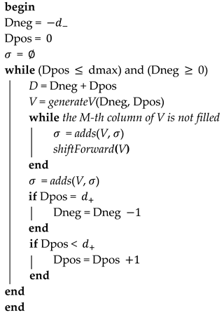
Then, we generate a degree-lexicographically organized set of monomials $\sigma$ of order $\mathcal{D}=\left[d_{-};d_{+}\right]$, where the power of each monomial lies within $\mathcal{D}$ and powers of each term in monomial also lies within $\mathcal{D}$. From a practical point of view, we assume that $d_{-}\le 0$ and $d_{+}\ge 0$. The algorithm for generating $\sigma$ is given in pseudocode in Listing 1.

The subroutine generateV returns a special indexing matrix V:

$$V=\left(\begin{array}{cc}\mathrm{Dpos}& \underset{\overbrace{\{\begin{array}{ccc} 1& 0& \begin{array}{cc}\dots & 0\end{array}\\ ⋮& ⋮& \begin{array}{cc}& \end{array}\\ 1& 0& \ddots \end{array}}}{M}\\ \mathrm{Dneg}& \{\begin{array}{ccc}-1& 0& \begin{array}{cc}& \end{array}\\ ⋮& ⋮& \begin{array}{cc}& \end{array}\\ -1& 0& \begin{array}{cc}\dots & 0\end{array}\end{array}\end{array}\right)$$

The subroutine adds produces a column-wise sum of $V$ as a candidate vector $\alpha ={\left({\alpha }_1,\dots ,{\alpha }_M\right)}^{\mathrm{T}}$ of monomial terms powers:

$$t\left(x\right)={\displaystyle \prod }_{i=1}^{M}x{ }_i^{{\alpha }_i}.$$

(33)

The monomial $t\left(x\right)$ is added to $\sigma$ if it is not already contained in $\sigma$. The order of multiplication is neglected, e.g., the term $x_1{x}_2{x}_1$ is considered similar to the term $x_1^2{x}_2$.

The subroutine shiftForward produces the next state of matrix $V_{k+1}=V_k\oplus$ 1 considering $V$ as a column-type of D-digit number in M-ary numeral system, where each digit has M states defined by the position of the non-zero element in each row, and where the first row is the least significant digit of the number, and $V_k\oplus$ 1 denotes summation with the column vector 1 $={\left(1,0,\dots ,0\right)}^{\mathrm{T}}$.

Listing 1. A pseudocode for a deglexord routine generating degree-lexicographically ordered Laurent monomials

When the degree-lexicographically ordered set of monomials $\sigma$ is computed, the Kera–Hasegawa method is applied to $\sigma$, $\mathbb{V}$, and $\mathbb{X}$. The obtained reconstructed PDS corresponds to the original dynamical system if the noise level in the data is sufficiently low and the system is representable in a form of PDS in a given set of coordinates.

3. Experimental Results

In this section, we first illustrate the advantages of using integral embedding using two examples and, then, show how the proposed approach can be used for the reconstruction of Lorenz attractor from a one-dimensional time series and chaotic memristive circuit equations from a three-dimensional time series.

3.1. Illustrations of the Theorems

The following example illustrates the Theorem 1.

Example 1.

Consider the ODE:

$$\{\begin{array}{c}\dot{x}=y, \\ \dot{y}=-x, \\ \dot{z}=f\left(x,y\right),\end{array}$$

(34)

where$f\left(x,y\right)=2 sign\left(x\right) \frac{y}{x^3}{e}^{-\frac{1}{x^2}}$. The solution of (30) is

$$\{\begin{array}{c}x=\sin \left(t\right),\hfill \\ y=\cos \left(t\right),\hfill \\ z=\mathrm{sign}\left(\sin t\right)e^{-\frac{1}{{\sin }^{2}t},}\hfill \end{array}$$

(35)

The function$z\left(t\right)$in (31) satisfies the conditions of the Theorem 1. Its unresolvable point is$x_0={\left(0,0,0\right)}^T$. Figure 3 shows two variants of 3-dimensional phase spaces, reconstructed via differentiation and integration from time series$\mathit{u}=\left\{z\left(t_i\right)\right\}$.

Example 2 shows how embedded differentiation and integration approaches can be applied to ECG signals. In this example, the conditions of both Theorems are satisfied, i.e., differentiation produces noisy trajectory reconstruction with a singular point, while integration does not have these drawbacks.

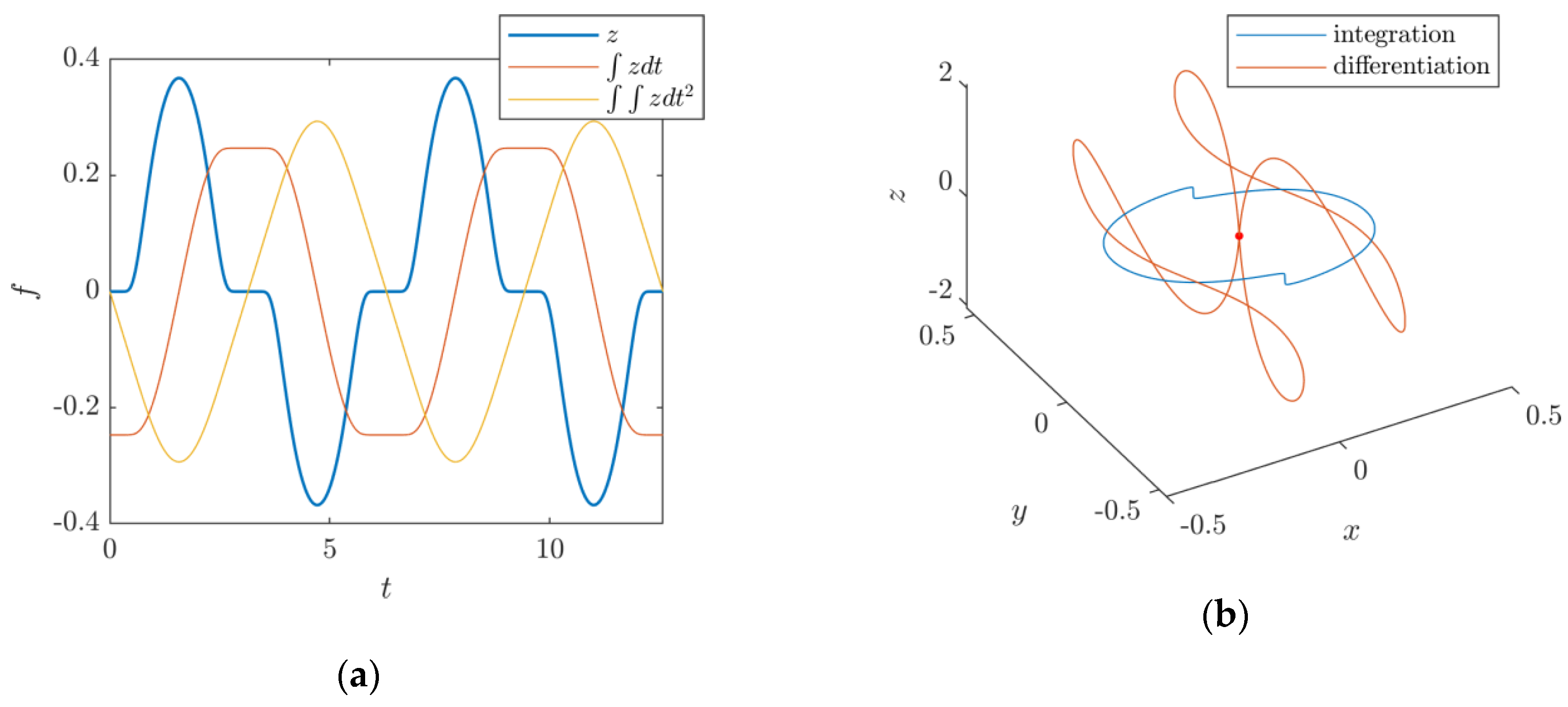
Example 2.

Consider the ECG signal from ECG-ID Database [30,31], as shown in Figure 4a.

After applying the embedded differentiation approach, we obtain a trajectory that does not satisfy the uniqueness criterion and is contaminated with noise. After applying embedded integration approaches, we obtain a rather a smooth trajectory with no singular points.

3.2. Reconstruction of Lorenz Attractor

Consider the classical Lorenz attractor

$$\{\begin{array}{c}\dot{x}=-sx+sy, \\ \dot{y}=-zx+rx-y,\\ \dot{z}=xy-bz, \end{array}$$

(36)

with a standard parameter set: $s = 10, r = 28, b = 8/3$ [32]. Suppose, only one variable $z$ can be observed, so we should transform the Lorenz system to obtain a model in new coordinates:

$$\{\begin{array}{c}{\dot{x}}_1=x_2,\hfill \\ {\dot{x}}_2=x_3,\hfill \\ {\dot{x}}_3=-s{x_1}^3-{x_1}^2{x}_2+bs(r-1)x_1-b(1+s)x_2-(1+b+s)x_3+\frac{x_2{x}_3}{x_1}+\frac{(s+1){x_2}^2}{x_1},\hfill \end{array}$$

(37)

Equation (37) cannot be reconstructed into ordinary polynomial functions due to the negative powers of variable $x_1$, but it is possible to reconstruct it as the Laurent polynomial function. The application of the proposed algorithm can be done using both differential and integration approaches.

The deglexord procedure (see Listing 1) generates a set of $L=50$ monomials or degrees $\mathcal{D}=\left[-1;3\right]$. To ensure that the system of equations is overdetermined, we should take not less than 51 points in $\mathbb{X}$. We are never sure that any term will vanish on $\mathbb{X}$ and will be removed by the ABM algorithm. An example of the reconstructed system is:

$$\{\begin{array}{c}{\dot{x}}_1=x_2,\hfill \\ {\dot{x}}_2=x_3,\hfill \\ {\dot{x}}_3=-10{x_1}^3+720x_1-{x_1}^2{x}_2-29.3333x_2-13.6667x_3+11{x_1}^{-1}{x_2}^2+{x_1}^{-1}{x}_2{x}_3,\hfill \end{array}$$

(38)

To reach a high quality of reconstruction, we generate data using the function ode113 with parameters RelTol $={10}^{-13}$ and AbsTol $={10}^{-15}$ and constant stepsize $h={10}^{-4}$and simulation time $T = 45$ in MATLAB 2019b environment (Campus license No. 40502181, ETU “LETI”) and use the 4th order integration formula. Note that Equation (37) can be reconstructed from the data obtained from the original Lorenz system using the time series corresponding to the variable $z$ and its two integrals.

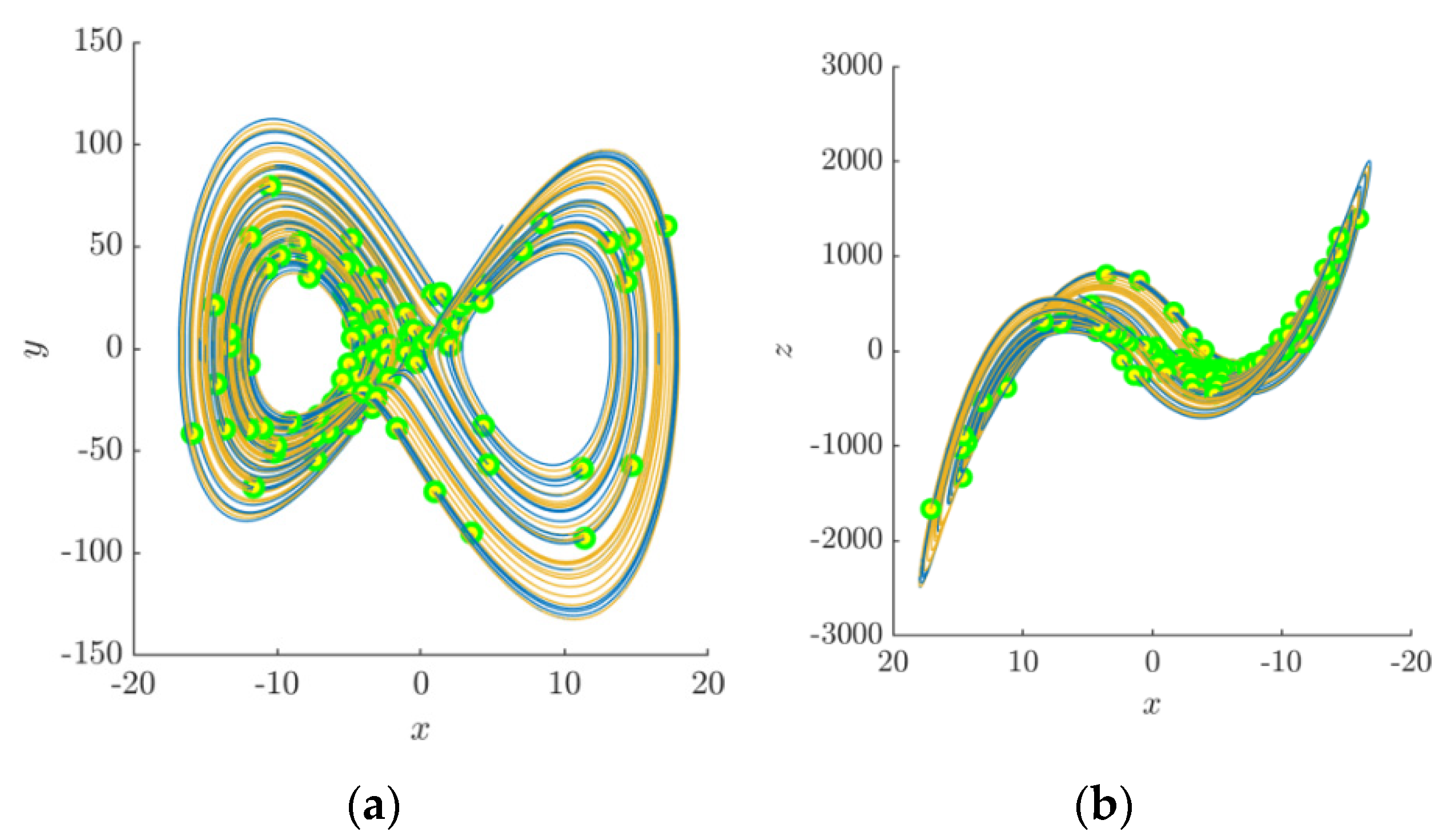
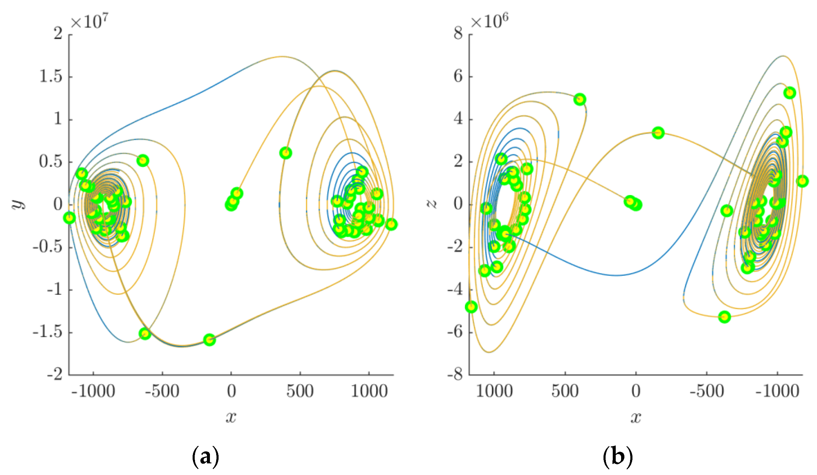
Two projections of the attractor Equation (37) and its reconstructed version are given in Figure 5. The initial conditions were ${\left(0.1,0,-0.1\right)}^{\mathrm{T}}$, the parameter $\eta ={10}^{-2}$.

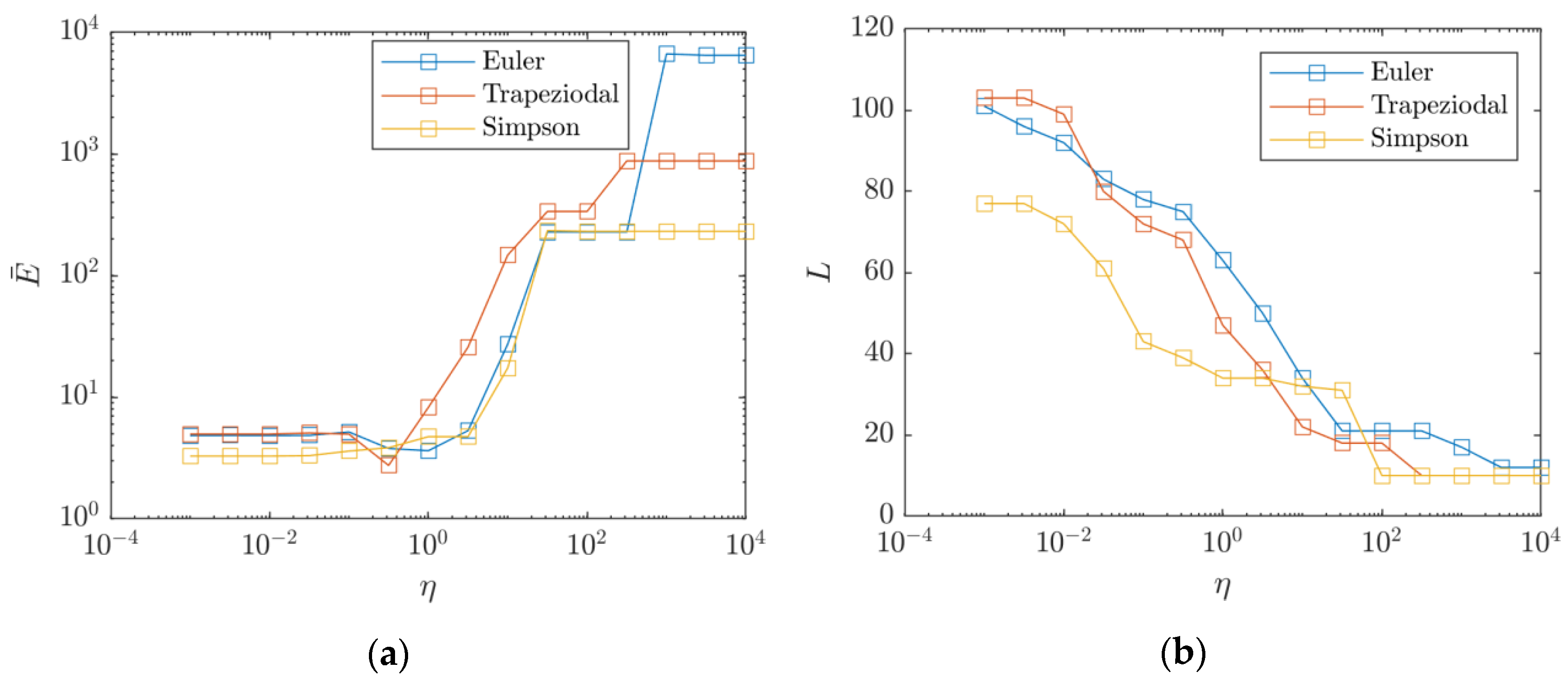
Truncation and round-off errors can be considered as a sort of noise [33] which makes it possible to compare differential embedding and integral embedding in terms of sensitivity to the reconstruction error induced by the stepsize. The results are given in Figure 6.

In Figure 6, we denote the phase space reconstruction method based on differentiation of the 2nd order of accuracy as DiffOrd2 (central differences) and of the 4th order of accuracy as DiffOrd4 (4 order finite differences) [34]. The method based on of 2nd order integration is denoted as IntOrd2 (trapezoidal rule) and the method of 4th order of accuracy is denoted as IntOrd4 (Simpson’s rule). Two plots summarize the results on mean error $E=\Vert v_k-H_k\left(\mathbb{X}\right)\Vert$ across three state variables and overall number of terms $L$.

We see from both plots that for small stepsizes, the integration based reconstruction method performs well while the differentiation approach suffers from numerical noise following with the proof of Theorem 2. The higher the sampling frequency is, the more noise is added into the data and the algorithm is more likely to fail. However, large stepsizes are more likely to corrupt the integration-based approach, but in this case this happens at $h>{10}^{-2}$when both methods give inaccurate results even on 4th order. The reconstruction techniques based on second-order formulae became inaccurate at $h>2.5 \cdot {10}^{-4}$, the fourth-order based formulae became inaccurate at $h>3.5 \cdot {10}^{-3}$. By “inaccurate” we mean that Equation (37) was reconstructed with some missing or excessive terms.

3.3. Reconstruction of Muthuswamy’s Memristive Circuit

Replacing the nonlinear negative resistor (Chua diode) in the well-known Chua’s circuit with the flux-controlled memristor one obtains a circuit able to exhibit the chaotic behavior [19]. The circuit proposed by B. Muthuswamy includes five elements (Figure 7): a linear passive inductor, two linear passive capacitors, a linear passive resistor and a nonlinear active memristor.

After scaling and transformation, we obtain the following system of ODEs:

$$\{\begin{array}{c}\dot{x_1}=p_1{x}_2,\hfill \\ \dot{x_2}=p_2\left(x_3-x_2\right)-p_3\left(\alpha +3\beta x_1^2\right)x_2,\hfill \\ \dot{x_3}=p_4\left(x_2-x_3\right)-p_5{x}_4,\hfill \\ \dot{x_4}=p_6{x}_3. \hfill \end{array}$$

(39)

Parameters for chaotic behavior are $\alpha =-0.667\cdot {10}^{-3}$; $\beta =0.029·{10}^{-3}$;$p_1=2.594·{10}^{-3}$;$p_2=73.53·{10}^3$;$p_3=147·{10}^6$;$p_4=7.353·{10}^3$;$p_5=14.7·{10}^6$;$p_6=\mathrm{55.55.}$ We simulated the system by the function ode113 with parameters RelTol $={10}^{-13}$ and AbsTol $={10}^{-15}$ and constant stepsize $h={10}^{-8}$ and final time $T = 0.01$. In this experiment we used data obtained from the original Equation (39) and reconstructed the state variable $x_1$ by integrating variable $x_2$. This is motivated by two facts: first, variable $x_1$ stands for the magnetic flux between the terminals of the memristive device [19], and therefore cannot be measured on a macroscopic scale, so it is assumed to be unobservable. Second, integrating $x_2$ is very natural to the system (39) due to the relation $\dot{x_1}=p_1{x}_2$ and therefore, needs no complicated transformations.

The degrees of terms in the monomials were placed within the interval $\mathcal{D}=\left[0;3\right]$, the tolerance parameter of AMB algorithm was $ϵ={10}^{-2}$. The reconstructed equations are

$$\{\begin{array}{c}{\dot{x}}_1=x_2,\hfill \\ {\dot{x}}_2=24519 x_2 + 73530 x_3 - 0.086055 x_1^2 x_2,\hfill \\ {\dot{x}}_3= 7353 x_2 - 7353 x_3 - 14700000 x_4,\hfill \\ {\dot{x}}_4=55.55 x_3.\hfill \end{array}$$

(40)

Note, that the Equations in (40) are a rescaled version of the Equations in (39) when ${\widehat{p}}_1=1$ instead of $p_1$ in the original equation.

Two projections of the attractor of original and reconstructed systems are given in Figure 8. The initial conditions were ${\left(0,0.1,0.1,0\right)}^{\mathrm{T}}$. We compared three integration methods by changing the tolerance parameter $\eta$ in the delMinorTerms algorithm in the range $\eta \in \left[{10}^{-3},{10}^4\right]$. Figure 9 depicts the result of the experiment. Using higher-order integration formulae allows for the achievement of more precise and more compact solutions. This experiment shows the difficulty of choosing $\eta$: its low values force the algorithm to generate equations with many excessive terms making the least-squares solution more precise. But, as one can see in Figure 9, the accuracy of the proper reconstruction is rather high due to high absolute values of the state variables (see Figure 6) and thus truncation and numerical errors in the reconstructed data for $x_1$ are large as well.

To summarize, the experiment shows that higher-order integration is more preferable and value $\eta$ should be adjusted with respect to the problem properties.

4. Discussion and Conclusions

Two main findings are highlighted in this paper. First, we show that the integral embedding approach has several advantages over the differential approach often used in cases of incompletely observed systems. Second, we extend the Kera–Hasegawa method to Laurent polynomials and show by example its performance.

Still, some limitations of this method exist. The first, and the most prominent one being, is that not each system can be represented as a PDS, and furthermore, there are some PDSs that do not allow transformation to the form of Equation (22) or Equation (24) or their combinations.

Consider the following system with an unobservable variable $z$:

$$\{\begin{array}{c}\dot{x }=y,\hfill \\ \dot{y}=-cx+by-by{z}^2,\hfill \\ \dot{z }=-y-az+yz,\hfill \end{array}$$

(41)

where $a,b,c$ are parameters. The natural way to reconstruct Equations (41) in this case is to transform it into

$$\{\begin{array}{c}\dot{x }=y,\hfill \\ \dot{y}=u,\hfill \\ \dot{u }=-cy+bu-\frac{u\left(by-cx-u\right)}{y}\pm 2by\sqrt{\frac{by-cx-u}{by}}\left(-y\pm \left(a-y\right) \sqrt{\frac{by-cx-u}{by}}\right),\hfill \end{array}$$

(42)

where a new variable $u$ is reconstructed from the observable variable $y$ through differentiation. Equation (42) cannot be represented in terms of polynomial functions and, moreover, needs a special technique to resolve the ambiguity in $\pm$ sign appearing when $z$ variable is expressed from the second Equation of (41).

The second limitation of the proposed reconstruction method can be exemplified by Muthuswamy’s memristive circuit. In many cases, the algorithm found a PDS different from Equations in (40), but which is also correct on limited data series $\mathbb{X}, \mathbb{V}$ and has a stable attractor similar to the attractor of the system Equations in (40):

$$\{\begin{array}{c}{\dot{x}}_1=x_2,\hfill \\ {\dot{x}}_2=24519 x_2 + 73530 x_3 - 0.086055 x_1^2 x_2,\hfill \\ {\dot{x}}_3= 35748530.2895 x_1+ 5895.007 x_2- 7353 x_3- 12770094.9573 x_4- 41.8226 x_1^3,\hfill \\ {\dot{x}}_4=55.55 x_3.\hfill \end{array}$$

(43)

Moreover, the third Equation in (43) is parametric, so infinitesimally many variants of it exist. So, if similar data can be produced by several PDSs, the method may find any one of them.

The third limitation of the proposed reconstruction method was found in both experiments with the Lorenz system and Muthuswamy’s memristive circuit, i.e., it is sensitive to algorithm parameters, such as stepsize, the order of accuracy of the reconstruction method, its type (differentiation or integration), and tolerance of delMinorTerms algorithm $\eta$. Obviously, sensitivity to the AMB algorithm tolerance $ϵ$ also takes place, but we did not investigate its influence.

The fourth limitation is that the dimension of search grows dramatically when the number of terms or system dimension grows. For example, four-dimensional PDS in complete Laurent polynomials containing degrees in $\mathcal{D}\in \left[-3,3\right]$ can be constructed out of 471 unique monomials, five-dimensional PDS out of 1281 unique monomials, and six-dimesional PDS out of 3067 unique monomials. Even if ABM algorithm sufficiently reduces these numbers, it is likely to obtain very poorly conditioned large-scale regression problems, and it is not obvious whether the algorithm remains useful in these cases. This question needs further investigation.

Laurent monomial ordering, delgexord, and BM algorithm for Laurent monomials also need the development of a stricter theoretical basement, as in the case of well-established ordinary monomials [35]. Moreover, from Equation (4) it is clear that the reconstruction approach based on the LSM can also handle not only PDSs but functions containing other elementary nonlinearities as well (e.g., trigonometric functions). This also needs further development.