1. Introduction
Exponential smoothing methods are widely used worldwide in time series forecasting, especially in financial and energy forecasting [
1,
2]. These methods smooth the observed values of a time series, using an exponentially downward weighting strategy giving more weight to recent values compared to older values. Weights decrease geometrically over past observations. The most commonly used methods are: Simple exponential smoothing for the series that does not show any trend, or with a locally stable mean, having a single smoothing parameter
α; double seasonal exponential smoothing (also known as Holt’s method [
3]) for trend-having series with two smoothing parameters:
α and
γ; finally, triple exponential smoothing (also known as Holt–Winters [
4]) for the series with a trend and seasonal component, with
α,
γ, and
δ as smoothing parameters. The smoothing parameters are bounded in the interval [0, 1], where the closer to 0 means the more weight of the old values against the newer ones.
The multiple seasonal Holt–Winters models (nHWT) outperform former Holt–Winters methods by including several seasonalities nested in the model. This development has been driven by the necessity of improving forecasts, especially in energy planning, where system operators need accurate forecasts. Hong [
5] determines how a 1% improvement in the forecast accuracy can save up to
$600,000 per year in a 1 GW power station.
However, these new forecasting methods are recursive and based on initial values, and the performance of the models highly depend on those initial values. Thus, new initialization methods to include multiple seasonality must be developed. Another question is then raised: Is there any method that outperforms the rest?
This article intends to provide answers to these questions. Hence, new initialization methods are proposed for nHWT models and their performance is analyzed for forecast accuracy by using the Spanish hourly electricity demand.
Holt–Winters models were formerly introduced in the 1960s and have been very commonly used in forecasting techniques and signal processing. The Holt–Winters model (also known as triple exponential smoothing) introduced by Winters [
4] consists of three smoothing equations and a forecasting equation as shown in Equations (1)–(4):
where
α,
γ, and
δ are the smoothing parameters, and
,
and
are the smoothing equations known as level, trend, and seasonality. The information from the observed values (
) is projected through a forecasting Equation (4) k steps ahead to obtain predictions (
).
Taylor [
6,
7] introduced the double and triple seasonal Holt–Winters models (HWT). These models are characterized by capturing the information contained in the seasonal component, split into several seasonalities of different lengths, as well as including an adjustment of the forecast including the first autocorrelation error. García-Díaz and Trull [
8] generalized these models to adapt to an indeterminate number of seasonalities, proposing the multiple seasonal Holt–Winters models (nHWT).
The trend and seasonal equations can be expressed in an additive or multiplicative form. The way the equations are combined allow a total of 30 possible combinations. The nomenclature used to name the models is based on three letters: The first to indicate the trend method, the second to indicate the seasonality method, and a third to indicate if the model has an adjustment using the first order autocorrelation error, as shown in
Table 1. Additionally, the seasonalities used are indicated by adding subscripts with period lengths.
The notation used is based on the following criteria: The first letter stands for the trend method (N: None, A: Additive, M: Multiplicative, d: Damped Additive, and D: Damped Multiplicative). The second letter stands for the seasonality method (N: None, A: Additive, and M: Multiplicative). The third letter is used to designate if the model has an AR (1) adjustment (C: Adjusted, L: Not adjusted).
As an example, the AMC
24,168 model is a model with an additive trend and multiplicative seasonality; the model is adjusted by using the first-order autocorrelation error, and it has two seasonalities: One daily (subscript 24) and one weekly (subscript 168). The equations defining the AMC
24,168 model are described in Equations (5)–(9). The general formulae of all possible models depending on the trend and seasonal type can be found in
Appendix A:
where the former seasonal equation
now splits into
and
δ splits into
,
being the seasonal periods considered,
and
. Here, the value
is the adjustment factor to include the first-order autocorrelation error (
).
The rest of the paper is organized as follows: In
Section 2, the previous literature is analyzed; in
Section 3 the initialization methods are described; in
Section 4, an analysis is carried out and the results obtained are described; and in
Section 5, these results are discussed.
Section 6 lists the conclusions reached.
2. Related Work
The Holt–Winters models are recursive, and thus an initialization value is needed to feed the model. With the development of new models, it is mandatory to define new initialization methods for obtaining the initial values of the smoothing equations, considering that the older methods were defined only for single seasonal models. These initialization methods also depend on the method used for trend and seasonality.
The first methods of obtaining initial values date back to the proposal made by Winters [
4] with the definition of triple exponential smoothing models. (Do not confuse triple exponential smoothing, with triple seasonal exponential smoothing, the former being a reference to the use of three equations, while the latter refers to the use of three seasonalities). In [
4], the initial value of the trend (
T0) is calculated as the slope between the average of the last available full period
q and the first, as indicated by Equation (10), where the only seasonality is of length
s.
Here, the value of
indicates the average value for the first period and
indicates the average value for the last period considered
q. In many cases, using the first two periods (that is,
q = 2) is sufficient [
9]. Granger and Newbold [
10] proposed leaving the trend in values of 0 for additive trend methods and 1 for multiplicative trend methods. In this way, the slope adjusts itself to the trend value.
The previous work of Holt [
3,
11] and Brown [
12] in single and double exponential smoothing did not require calculations of initial values external to the model. Makridakis, Wheelright, and Hyndman [
9] proposed a new method of calculating the trend and seasonality. Bowerman, O’Connell and Pack [
13], and Bowerman, O’Connell, and Köhler [
14] proposed a regression method where they consider that the intercept is the level and the slope is the trend. This method is criticized by Hyndman [
15] for the bias it introduces. Rasmussen [
16] proposed obtaining initial values through minimization. With the emergence of multiple seasonal models, new initialization methods were introduced [
6,
7], although some authors prefer not to use them [
17]. Taylor introduced a new initialization method of the level and trend applied to double seasonal Holt–Winters in [
6]. In particular, the seasonality is initialized as the division of the simple values over the moving average of the period (called the “simple” method), and the level (S
0) is obtained once the series trend has been eliminated. It consists in first obtaining the trend of the series and then the level, as seen in Equation (11):
where
is the longest seasonality. This scheme to initialize the level was also adopted by Hyndman et al. [
18]. Hyndman introduced new initialization methods incorporated in the exponential smoothing methodology based on state spaces and included them in the “forecast” package of the statistical software R. Trull, García-Díaz, and Troncoso [
19] also used a series decomposition using STL methods of various seasonality, in order to obtain initial values in discrete seasonality.
Some papers [
20,
21,
22] analyze the initial values but very succinctly. Segura and Vercher [
23] collect the information about the initialization methods and perform an analysis similar to that carried out by Makridakis and Hibon [
24]. They conclude that when the parameters are optimized, it is not possible to determine significant differences between the different initialization methods.
After an exhaustive review of these previously published works, it can be concluded that the analysis of the initialization methods is not very extensive in the literature. This fact justifies the need for research in the topic described in this paper.
3. Materials and Methods
The way to obtain the initial values must match the trend and seasonal method, as it would impact later on the accuracy of the model. The addition of more seasonal patterns in the model requires newer methods of obtaining the initial values or seeds. Therefore, several methods depending on the trend and seasonal method have been implemented. This paper proposes new initialization methods for multiple seasonalities based on the previous methods, which were defined for a single seasonal pattern.
The proposed methods for the initialization of the Holt–Winters models are separated into three groups. The first ones calculate the seeds for the level and trend separately. The last one implements each seasonality separately. The latter first obtains a seed, as the trend, and then obtains another one on a recurring basis, such as that of the level.
3.1. Level Methods
The level initialization basically consists in determining the longest period, or the longest seasonality (
) and determining the initial values around that point, by using the moving average (adapted from Holt [
3]) or the average (adapted from Winters [
4]). Williams and Miller [
25] used the first value of the series for the level. This method is included although it remains unchanged for the further comparative analysis in
Section 4.
Table 2 shows the adapted methods to obtain the initial value of the level (
).
3.2. Trend Methods
Based on Winters’ method [
4], a new initialization method has been developed to be able to include more than one seasonality in the model, according to the contribution to the trend of smaller seasonality, as indicated [
24]. These proposals (methods overall and two periods) are shown in
Table 3 along with the methods published in [
6,
26] for the further comparative analysis in
Section 4.
is an intermediate step where individual contributions are calculated in each period of length
. The average of all of them will be taken into account, counting the maximum number of periods q for the overall case, and only two periods for that special case (
). The seasonality of greater length is used as the basis of calculation. The value of
indicates the length of the longest seasonal period considered in the model. The rest is calculated in the form of differences. The value
indicates the length of the minor of the periods considered.
indicates differences in values for the first two periods, while
refers to differences in the period considered. Finally, the average of the contributions is calculated to obtain the value of
.
3.3. Seasonality Calculation Methods
The first methods determined for the calculation were developed by Winters [
4]. The calculation of seasonality consists in calculating the series averages over the series without a trend. When it comes to more than one seasonality that are modeled annually, as in nHWT, it is necessary to avoid duplication of the effects of seasonality. Thus, based on Winters’ method [
4], we propose to obtain the seasonal indices
for each seasonality (
) of length
as described in Equations (12)–(16):
with the individual seasonal indices,
where
is the maximum number of complete cycles of length
that exist in the series.
refers to the seasonality considered, so that
.
Brockwell and Davis [
27] proposed another method, in which the calculation of seasonality is done by obtaining the weights of the series against the average values of the cyclic pattern. This methodology is adopted by the National Institute of Standards and Technology (NIST) [
28]. This method has also been adapted to multiple seasonality, and the proposed method is described in the following steps:
Step 1:
For each seasonality, it is necessary to reorganize the data and obtain the means in each internal position within the seasonality as the average of the values obtained. In this way, the values
are obtained, for each seasonality of length
and that occurs
times in the data series, as shown in Equation (17):
Step 2:
For each seasonality, the proportion of the series over the average is obtained. There are
occurrences of seasonal cycles in the range considered of length
.
| | 1 | 2 | … | q |
| 1 | | | | |
| … | | | | |
| | | | |
Step 3:
The provisional seasonal indices of each seasonality on the series are obtained as follows:
Step 4:
The definitive seasonal indices, shown in Equation (18) are obtained taking into account that they are nested, and therefore the seasonal indices by removing the first one, need to compensate for the effect produced in the indices considered prior to the one calculated.
Finally, the initialization method proposed by Granger and Newbold [
26], named the “normal” method, has been adapted, where the values of the first cycle are divided by their average. This proposal is described by Equations (19) and (20):
4. Results
The proposed new methods and older methods published in [
6,
25,
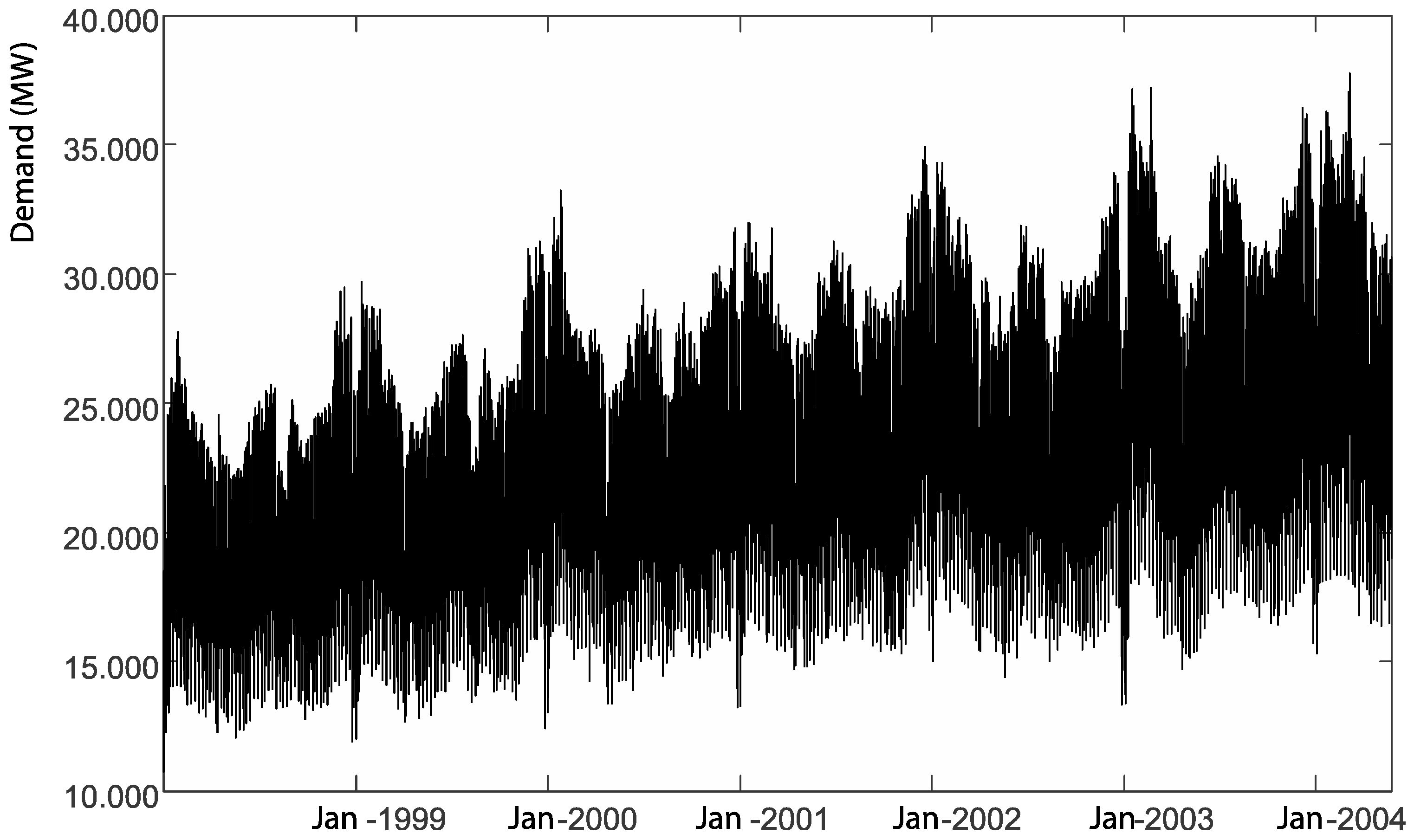
26] were applied to the hourly electricity demand series in Spain in the period 1999 to 2004.
Figure 1 shows the time series worked. This period is characterized by strong continued growth and marked seasonality. This will allow working with models with clear seasonality and trend.
The analysis has been raised in the form of an experimental design. The main factors to analyze are the different methods to estimate the initial values of level, trend, and seasonality. It has been used as two seasonal patterns. It is important to note that, when performing this analysis, the influence of the meteorological variables has been considered as a noise factor, so that windows have been created in the four seasons of the year where the analysis was performed. Within the same context, several replicas of the analysis have been included, using the different years.
The response variables used were the MAPE (see Equation (20)), an indicator of forecast accuracy widely used in the time series analysis [
29]. To obtain the response variable, the seven-week series have been used randomly extracted from the series, although always taking into account that they belong to a specific season of the year—having at least six series in each seasonal period and each year.
The process of comparing the initial values needs a specific methodology, since once the parameter optimization is performed, the differences between them are lost [
9,
24]. This situation can be avoided by performing the analysis based on the forecasts directly from the initial values and without adjusting. It is also necessary that the model does not cushion the results, which implies that the parameters used must be
and
for all seasons.
Table 4 shows all methods both proposed and published in the literature that will be used to initialize the level, trend, and seasonality factors of nHWT models.
The names used are consistent with the methods presented in the previous section. In addition, they have been carried out in four different years, which is an additional factor to consider. The models studied have been , , and .
The design of experiments includes 4096 tests, three controllable multilevel factors, and a noise factor that is the period of the year replicated for four different years. This study is shown in
Table 5.
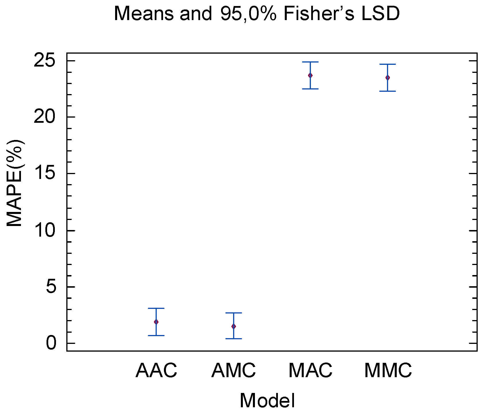
The first action taken, regardless of the design, was to be clear if there are significant differences between the models and from there determine which options to use. The result is shown in
Figure 2, where you can see how the groups with additive trend differ significantly from the groups with multiplicative trend. Thus, the design will be separated in two to address each trend by its side.
Table 5 shows the results of the ANOVA (analysis of variance) obtained during the design. Only those significant factors and interactions are shown. This ANOVA has been carried out using the models with multiplicative trend and in response to the MAPE.
It is appreciated how the use of different seasonal methods is not significant, while the rest of the factors are. This model is also able to minimize the effect of the seasons of the year, becoming a nonsignificant factor, due to the influence of the trend being superior to that of the other parameters.
The same analysis performed on the models with additive trend offers slightly different results.
Table 6 shows the ANOVA of this analysis. Only the significant factors and interactions are shown. The behavior is similar, although the additive trend methods are more sensitive to the annual period considered and the seasonality method considered.
The analysis for each factor is shown in the graphs of
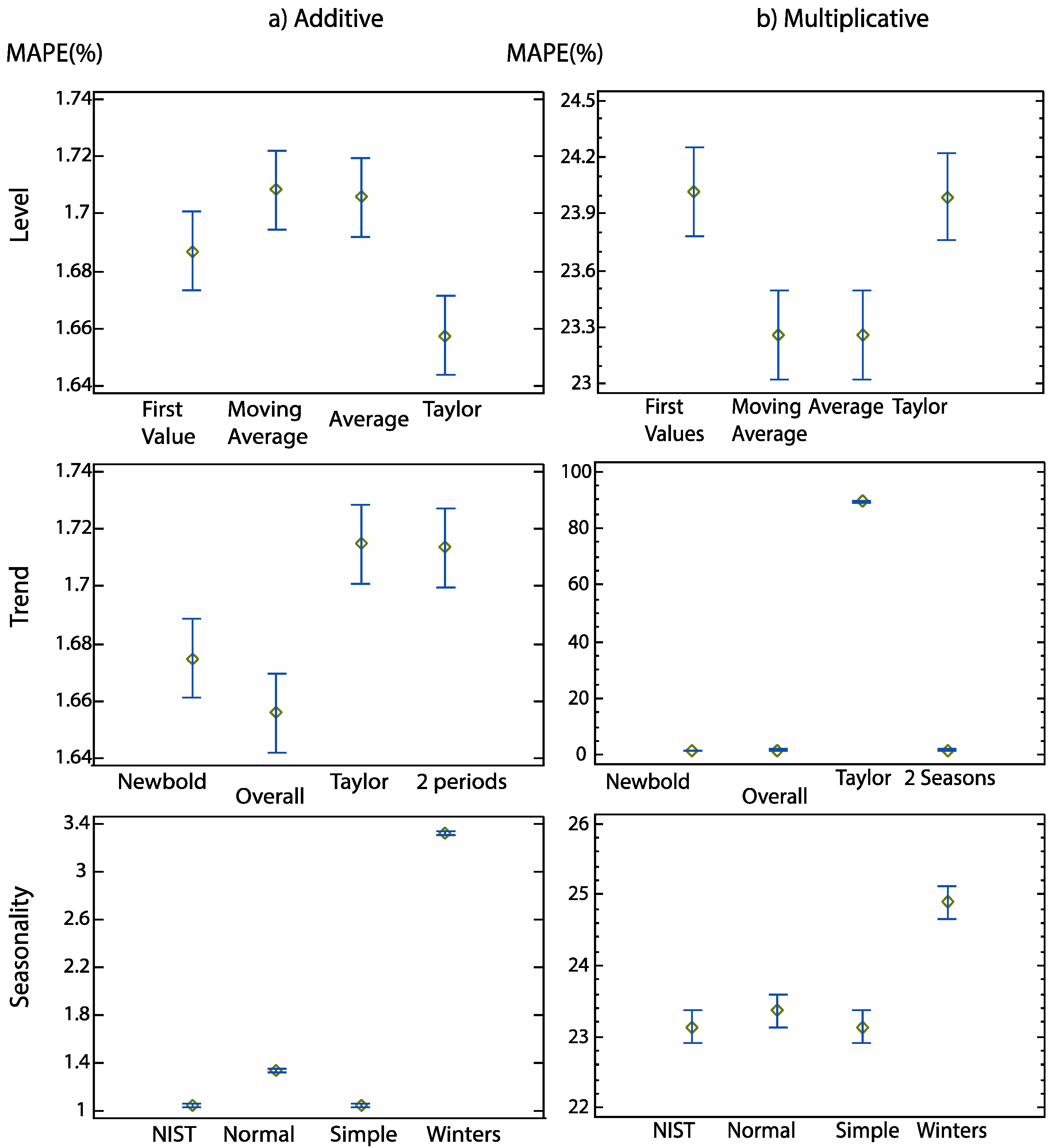
Figure 3. This figure shows the average graphs of the different factors separated by the trend method. MAPE (%) is displayed before optimizing. You can see how the behaviors are different depending on the trend. For those with multiplicative trend only the method proposed by Taylor is significantly different, both for the level and for the trend, but not for the seasonality. However, for additive trend methods, there are differences in all cases. Seasonal values in additive trend methods show differences between them, with the simple method and NIST being the best results.
Following these results, the values obtained during the experiment were analyzed, and each of the analyzed factors was studied separately.
4.1. Trend Analysis
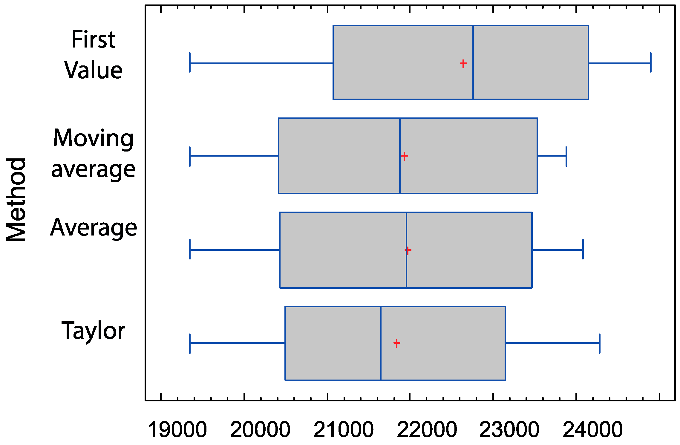
The trend determines the behavior of the series in the long term. Using the seven-week series, this influence is remarkable. The models that include multiplicative trend obtain results for the trend close to 1. It is difficult to assess this situation. However, with the additive trend models, more information can be obtained. The distribution of the initial values for the additive trend is shown in
Figure 4. It should be noted that the initial value of the Newbold method is always 0, and that the overall method has little variability. This is not the case with the two-period method. This tells us that the larger the set of data we take for the calculation of initial values, the more the variability is reduced.
Taylor’s method has a different behavior. Its variability is much greater than the rest. This is in contrast to using only the first two periods, in addition to introducing the contribution of the minor seasonality to obtain the overall trend.
4.2. Level Analysis
The analysis on the level shown in
Figure 5 reveals that the level values in the additive trend models are close. However, following what has been verified in the ANOVA, they are clearly significant when determining the accuracy of the model. The fact that Taylor’s method for the level is mixed, and that the trend has been previously calculated, causes this method to decrease variability, transferring it to the trend. For cases of multiplicative trend, the results are very similar to those obtained in this analysis.
4.3. Seasonality Analysis
The ANOVA indicates that there are significant differences only in the additive trend models. Therefore, this analysis focuses on these models. There are two large groups between which you can include the original adapted Winters method: The NIST method and the simple adapted one. The analysis focuses on these two methods—simple and Winters—and the results obtained with the AMC
24,168 model have been used. Therefore, the initial values for the 24- and 168-hour length seasonality are shown.
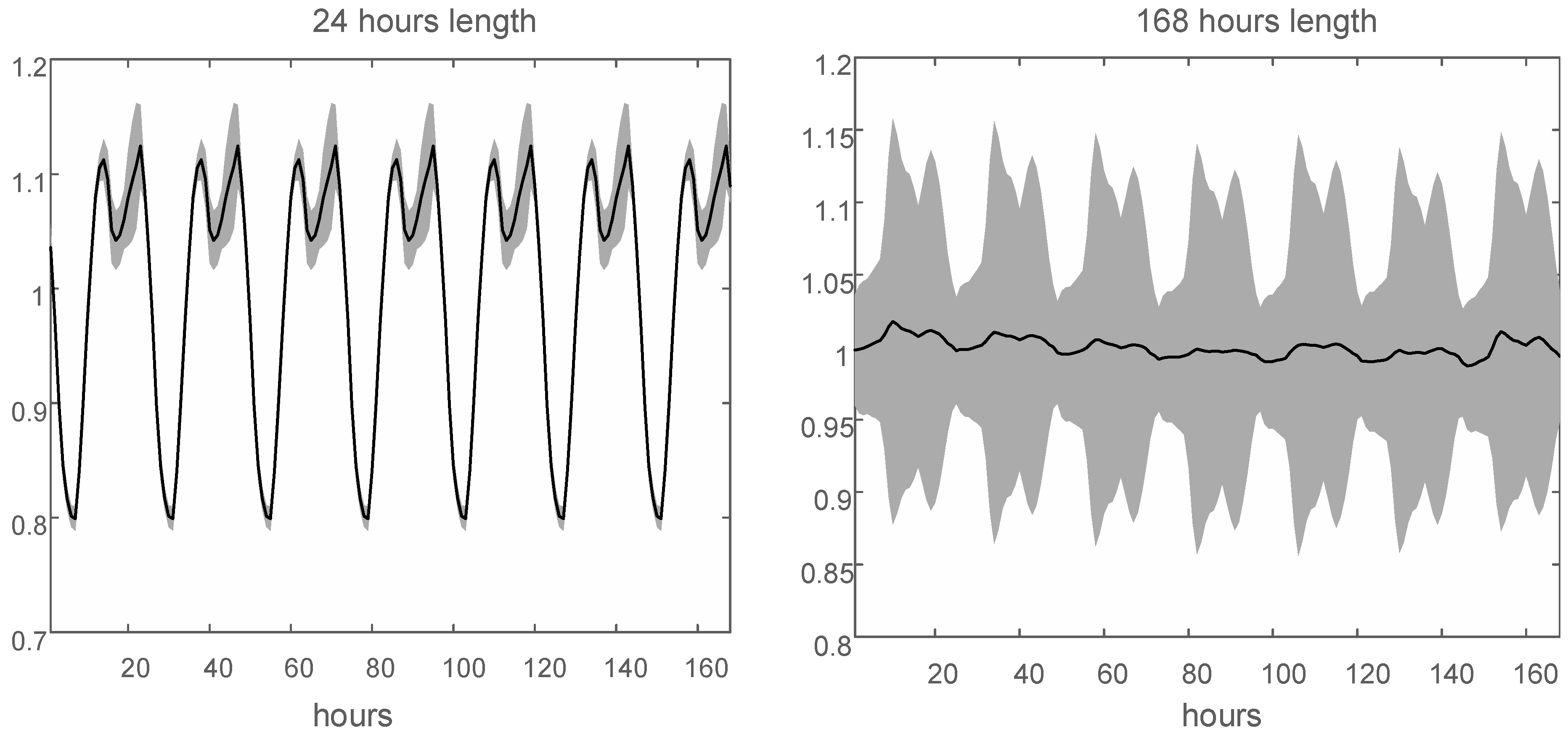
Figure 6 shows the distribution of the initial values for these seasonalities using the simple method. Similarly,
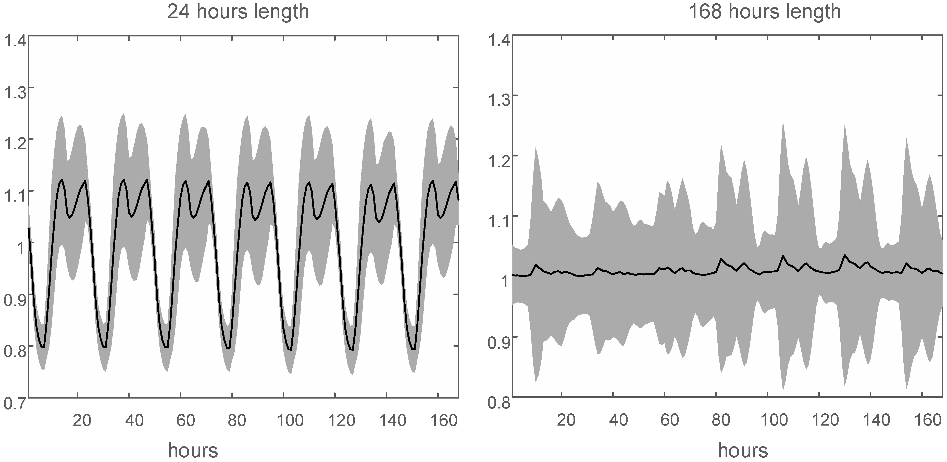
Figure 7 reflects this same distribution but using the Winters method.
It can be seen how the simple method has a lower variability in obtaining the seasonal indices of 24 hours, which is accompanied by a lower variability in the seasonal index of 168 hours. This indicates that the simple method ensures that the initial values are better suited to the seasonal patterns shown in the series. That is why it shows a smaller MAPE series. Moreover, you can see how the daily seasonal index is the primary index, and the weekly index has to be adapted according to the series. You might think that this situation occurs by the method of obtaining the initial values, where the first seasonality is considered the daily seasonality. However, we have performed tests where the first seasonality considered is the weekly one, and the results are the same.
5. Discussion
As a result of the analyses carried out in the study, it can be seen how the use of one or another method of obtaining initial values can greatly affect the accuracy of the forecasts. Although once the values of the parameters are optimized, these differences can be minimal (as other authors already describe), their influence on accuracy is clear. As a consequence, the parameters may not be optimal starting from unsuitable initial values, which complicates the optimization of the model in the adjustment, and later, in the forecasts.
The first impression is to see how multiplicative trend models start with a much higher MAPE than additive trend models do. In principle, it could be thought that it is due to the trend method used, but if the MAPE values are observed in
Figure 3b, it is observed how this is not the case, but the accuracy is worsened by the rest of the equations with the trend. Clearly, the work of the parameters in this case is to mitigate the effect of the initial seasonal and level values. It has also been observed that the result of the MAPE depends a lot on the trend and seasonality methods used. This does not mean that one method is better than another method, but there are differences between them at the initial state that the model must deal with. For each group of methods, we tried to locate differences within the trend, level, and seasonal methods, looking for the MAPE of the model without optimizing. The cases of multiplicative trend, for example, do not show large differences between initialization methods. On the contrary, the methods that use the additive trend do show a great dependence on how to obtain the initial values. Another factor to highlight is the behavior of seasonal indices. Depending on the method, a greater or lesser variability can be observed.
Thus, for the multiple seasonal methods of additive trend it is proposed to use the Taylor method for the level, the overall method for the trend, and the simple method or that of the NIST for seasonality. For models with a multiplicative trend, the use of the average method for the level, the Granger and Newbold method for the trend, and any of the methods proposed for seasonality are proposed.
6. Conclusions
In this article, we have presented new methods of obtaining initial values for multiple seasonal Holt–Winters models. These methods are based on the adaptation of existing methods for models with a single seasonality. In addition, a comparative analysis between our proposals and well-known methods published in the literature has been carried out in order to determine their influence on the accuracy of the models. All these initialization methods have been applied to the prediction of the electricity demand time series in Spain, in a period between 1999 and 2004. The characteristics of the series allow all methods to be analyzed effectively. An experimental design has been performed in which MAPE has been analyzed as a response variable, using the different initialization methods of the smoothing equations as factors to influence the response variable. The results show that the influence of the methods of obtaining initial values is greater on multiple seasonal Holt–Winters models with an additive trend. Finally, and based on the results obtained, a proposal on which method of initialization to use has been made.
