Existence Results for Nonlinear Fractional Problems with Non-Homogeneous Integral Boundary Conditions

Abstract

This paper deals with the study of the existence and non-existence of solutions of a three-parameter family of nonlinear fractional differential equation with mixed-integral boundary value conditions. We consider the $\alpha$-Riemann-Liouville fractional derivative, with $\alpha \in (1,2]$. To deduce the existence and non-existence results, we first study the linear equation, by deducing the main properties of the related Green functions. We obtain the optimal set of parameters where the Green function has constant sign. After that, by means of the index theory, the nonlinear boundary value problem is studied. Some examples, at the end of the paper, are showed to illustrate the applicability of the obtained results.

1. Introduction

In recent years, fractional calculus has been applied to a huge number of fields in science, engineering, and mathematics. Some of the areas where fractional calculus has made a profound impact include biology, physics, viscoelasticity, rheology, electrical, engineering, electrochemistry and control theory, see for instance [1,2,3,4,5,6,7].

Integral boundary conditions have been considered, for instance, in [8], where various applications in applied fields such as chemical engineering, thermoelasticity, population dynamics are explained.

The existence of solutions of nonlinear boundary value problem coupled with integral boundary conditions in ordinary and fractional cases has been widely studied by many authors, see for example [9,10,11,12,13,14] and the references therein. In 2009, Ahmad and Nieto [15] obtained some existence results for the following nonlinear fractional integrodifferential equations with integral boundary conditions:

$$\begin{array}{c}\hfill \left\{\begin{array}{c}{}^C{D}^{q}x\left(t\right)=f(t,x\left(t\right),\left(\chi x\right)\left(t\right)),0<t<1,1<q\le 2,\hfill \\ \alpha x\left(0\right)+\beta x^{\prime }\left(0\right)={\int }_0^1{q}_1\left(x\left(s\right)\right)ds,\hfill \\ \alpha x\left(1\right)+\beta x^{\prime }\left(1\right)={\int }_0^1{q}_2\left(x\left(s\right)\right)ds,\hfill \end{array}\right.\end{array}$$

where $f:[0,1]\times X\times X⟶X$, for $\gamma :[0,1]\times [0,1]⟶[0,\infty )$,

$$\left(\chi x\right)\left(t\right)={\int }_0^t\gamma (t,s)x\left(s\right)ds,$$

$q_1,q_2:X⟶X$$\alpha \ge 0$, $\beta \ge 0$ are real numbers and X is a Banach space, by employing to Guo-Krasnoselskii fixed-point theorem and contraction mapping principle.

In [16], it is studied the following nonlinear problem involving nonlinear integral conditions:

$$\begin{array}{c}\hfill \left\{\begin{array}{c}{}^C{D}^{\alpha }y\left(t\right)=f(t,y\left(t\right)),t\in [0,T],1<\alpha \le 2,\hfill \\ y\left(0\right)-y^{\prime }\left(0\right)={\int }_0^{T}g(s,y\left(s\right)ds,\hfill \\ y\left(T\right)-y^{\prime }\left(T\right)={\int }_0^{T}h(s,y\left(s\right))ds.\hfill \end{array}\right.\end{array}$$

Here, $f,g$ and $h:[0,T]\times E⟶E$ are given functions that satisfy suitable assumptions and E is a Banach space. By means of the technique associated with measures of non-compactness and the fixed-point theorem of Monch type, it is proved the existence of solutions of the problem.

In [17], it is considered the following nonlinear fractional differential equations with boundary value conditions

$$\begin{array}{c}\hfill \left\{\begin{array}{c}{D}^{\alpha }u\left(t\right)+g\left(t\right)f(t,u\left(t\right))=0,0<t<1,\hfill \\ u\left(0\right)=0,u^{\prime }\left(1\right)={\int }_0^{1}h\left(t\right)u\left(t\right)dt,\hfill \end{array}\right.\end{array}$$

where $1<\alpha \le 2$, $g\in C\left(\right(0,1),[0,\infty \left)\right)$ and g may be singular at $t=0$ or/and at $t=1$, $h\in L^1[0,1]$ and $f\in C[0,1]\times [0,1],[0,\infty ))$. The authors derive the Green function associated with the above problem and sharp estimates on it are established. Thus, by using fixed-point theorem in cones, they proved some results on the existence of positive solutions.

In this paper, the following nonlinear fractional differential equation with non-homogeneous integral boundary conditions is considered:

$$\begin{array}{c}\hfill \left\{\begin{array}{c}{D}^{\alpha }u\left(t\right)-\lambda u\left(t\right)+f(t,t^{2-\alpha }u\left(t\right))=0,t\in I:=[0,1],\hfill \\ \underset{t\to 0^{+}}{lim}{t}^{2-\alpha }u\left(t\right)=\mu {\int }_0^{1}u\left(s\right)ds,u^{\prime }\left(1\right)=\eta {\int }_0^{1}u\left(s\right)ds.\hfill \end{array}\right.\end{array}$$

(1)

Here $\lambda \in \mathbb{R}$, $\mu ,\eta \ge 0$, $D^{\alpha }$, $1<\alpha \le 2$, is the Riemann-Liouville fractional derivative and $f\in C\left(\right[0,1]\times [0,\infty ),[0,\infty \left)\right)$.

We look for solutions $u:I\to \mathbb{R}$ such that function $t^{2-\alpha }u\left(t\right)\in C^1\left(I\right)$. Thus, as a direct consequence, we deduce that, in particular, $u\in C^1\left((0,1]\right)$. Moreover, it may be discontinuous at $t=0$.

We are interested in to prove the existence and non-existence of solutions of the treated problem. To this end, we will use the classical index theory [18,19,20], in the line of the papers [21,22,23,24,25], where it is used for ordinary differential equations.

The main tool is the construction of the Green function related to the corresponding linear problem

$$\begin{array}{c}\hfill \left\{\begin{array}{c}{D}^{\alpha }u\left(t\right)-\lambda u\left(t\right)+y\left(t\right)=0,t\in I,\hfill \\ \underset{t\to 0^{+}}{lim}{t}^{2-\alpha }u\left(t\right)=\mu {\int }_0^{1}u\left(s\right)ds,u^{\prime }\left(1\right)=\eta {\int }_0^{1}u\left(s\right)ds.\hfill \end{array}\right.\end{array}$$

(2)

It is important to mention that the results obtained in [26] are fundamental in the development of our results. In such reference we consider the homogeneous case $\mu =\eta =0$, i.e., with no integral boundary conditions. There, we obtain the explicit expression of its related Green function (denoted by $G_1$ on this paper). Moreover, we deduce some sharp properties concerning its constant sign, compiled on Lemmas 1 and 2. The main properties of the Green function G related to the considered problem (2) are derived from the ones proved in [26] for $G_1$. Therefore, we use the qualitative properties obtained on those reference and study the parameter relationship between $\alpha ,\lambda ,\mu$ and $\eta$ that ensure the constant sign of the Green function related to the linear problem (2). We follow similar arguments to the ones used on [12,27,28,29,30].

The paper is scheduled as follows: after some introductory results, we study, in Section 3, the related linear equation and deduce suitable properties on the qualitative behavior and constant sign of the related Green function. Next section is devoted to ensuring the existence and non-existence of solutions of the considered nonlinear boundary value problem. The results follow from index theory. Finally, in last section, some examples are given to point out the applicability of the obtained results.

2. Preliminary Results

In this section, we introduce some notations and definitions that which we need in later.

Definition 1

([31]). The Riemann-Liouville fractional integral of order $\alpha >0$ for a measurable function $f:(0,+\infty )\to \mathbb{R}$ is defined as

$$I^{\alpha }f\left(t\right)=\frac{1}{\mathsf{\Gamma }\left(\alpha \right)}{\int }_0^t{(t-s)}^{\alpha -1}f\left(s\right)ds,t>0,$$

where Γ is the Euler Gamma function, assuming that the right-hand side is point-wise defined on $(0,+\infty ).$

Definition 2

([31]). The Riemann-Liouville fractional derivative of order $\alpha >0$ for a measurable function $f:(0,+\infty )\to \mathbb{R}$ is defined as

$$D^{\alpha }f\left(t\right)={\displaystyle \frac{1}{\mathsf{\Gamma }(n-\alpha )}}{\left(\frac{d}{dt}\right)}^n{\int }_0^t{(t-s)}^{n-\alpha -1}f\left(s\right)ds={\left(\frac{d}{dt}\right)}^n{I}^{n-\alpha }f\left(t\right),$$

provided that the right-hand side is point-wise defined on the interval $(0,+\infty )$. Here $n=\left[\alpha \right]+1$, where $\left[\alpha \right]$ denotes the integer part of the real number α.

Let $C\left(I\right)$ be the Banach space of all continuous functions defined on I endowed with the maximum norm $\parallel f\parallel =:max\left\{\right|f\left(t\right)|:t\in I\}$. Define for $t\in I$, $f_{\gamma }\left(t\right)=t^{\gamma }f\left(t\right)$, if $t>0$ and $f_{\gamma }\left(0\right)={lim}_{t\to 0^{+}}{t}^{\gamma }f\left(t\right)$, provided it exists. Let $C_{\gamma }\left(I\right)$, $\gamma \ge 0$ be the space of all functions f such that $f_{\gamma }\in C\left(I\right)$. It is well known that $C_{\gamma }\left(I\right)$ is a Banach space endowed with the norm

$${\parallel f\parallel }_{\gamma }=:max\{t^{\gamma }\left|f\left(t\right)\right|:t\in I\}.$$

3. Linear Problem

This section is devoted to the study of the linear problem (2). More concisely, we deduce the exact values of the parameter $\lambda$ for which the Green function G satisfies a strong positiveness condition. In a first moment we introduce the concept of Mittag-Leffler function.

Definition 3

([31], p. 42). A two-parameter function of the Mittag−Leffler $E_{\alpha ,\beta }\left(x\right)$ is defined by the series expansion

$$E_{\alpha ,\beta }\left(x\right)=\sum _{k=0}^{\infty }\frac{x^k}{\mathsf{\Gamma }(\alpha k+\beta )},\alpha ,\beta >0,x\in \mathbb{R}.$$

For $\beta =1$, $E_{\alpha ,1}$ coincides with the usual Mittag−Leffler function $E_{\alpha }$.

It is not difficult to verify that, provided $E_{\alpha ,\alpha -1}\left(\lambda \right)\ne 0$,

$$v_1\left(t\right)=\mathsf{\Gamma }(\alpha -1)\left(t^{\alpha -2}{E}_{\alpha ,\alpha -1}\left(\lambda t^{\alpha }\right)-\frac{E_{\alpha ,\alpha -2}\left(\lambda \right)}{E_{\alpha ,\alpha -1}\left(\lambda \right)}{t}^{\alpha -1}{E}_{\alpha ,\alpha }\left(\lambda t^{\alpha }\right)\right)$$

(3)

is the unique solution of the problem

$$\begin{array}{c}\hfill \left\{\begin{array}{c}{D}^{\alpha }{v}_1\left(t\right)-\lambda v_1\left(t\right)=0,t\in I,\hfill \\ \underset{t\to 0^{+}}{lim}{t}^{2-\alpha }{v}_1\left(t\right)=1,v_1^{\prime }\left(1\right)=0,\hfill \end{array}\right.\end{array}$$

(4)

and

$$v_2\left(t\right)=\frac{t^{\alpha -1}{E}_{\alpha ,\alpha }\left(\lambda t^{\alpha }\right)}{E_{\alpha ,\alpha -1}\left(\lambda \right)}.$$

(5)

the unique one of

$$\begin{array}{c}\hfill \left\{\begin{array}{c}{D}^{\alpha }{v}_2\left(t\right)-\lambda v_2\left(t\right)=0,t\in I,\hfill \\ \underset{t\to 0^{+}}{lim}{t}^{2-\alpha }{v}_2\left(t\right)=0,v_2^{\prime }\left(1\right)=1.\hfill \end{array}\right.\end{array}$$

(6)

Moreover, as it is showed in Theorem 6 in [26], if $E_{\alpha ,\alpha -1}\left(\lambda \right)\ne 0$, the unique solution of problem

$$\begin{array}{c}\hfill \left\{\begin{array}{c}{D}^{\alpha }v\left(t\right)-\lambda v\left(t\right)+y\left(t\right)=0,t\in I,\hfill \\ {\displaystyle \underset{t\to 0^{+}}{lim}{t}^{2-\alpha }v\left(t\right)=v^{\prime }\left(1\right)=0,}\hfill \end{array}\right.\end{array}$$

follows the expression

$$v\left(t\right)={\int }_0^1{G}_1(t,s)y\left(s\right)ds,$$

with

$$\begin{array}{c}\hfill G_1(t,s)=\left\{\begin{array}{c}\frac{t^{\alpha -1}{E}_{\alpha ,\alpha }\left(\lambda t^{\alpha }\right)E_{\alpha ,\alpha -1}\left(\lambda {(1-s)}^{\alpha }\right)}{{(1-s)}^{2-\alpha }{E}_{\alpha ,\alpha -1}\left(\lambda \right)}-{(t-s)}^{\alpha -1}{E}_{\alpha ,\alpha }\left(\lambda {(t-s)}^{\alpha }\right),0\le s\le t\le 1,\hfill \\ \frac{t^{\alpha -1}{E}_{\alpha ,\alpha }\left(\lambda t^{\alpha }\right)E_{\alpha ,\alpha -1}\left(\lambda {(1-s)}^{\alpha }\right)}{{(1-s)}^{2-\alpha }{E}_{\alpha ,\alpha -1}\left(\lambda \right)},0\le t<s<1.\hfill \end{array}\right.\end{array}$$

(7)

In order to characterize the uniqueness of solutions of Problem (2), we denote (See Figure 1 and Figure 2)

$$\theta \equiv \theta (\alpha ,\lambda ):={\int }_0^1{v}_1\left(t\right)dt\mathrm{and}\sigma \equiv \sigma (\alpha ,\lambda ):={\int }_0^1{v}_2\left(t\right)dt.$$

Theorem 1.

Let $y\in C(0,1]\cap L^{\infty }(0,1)$, $1<\alpha \le 2$, $\mu ,\eta \ge 0$ and $\lambda \in \mathbb{R}$ be such that $E_{\alpha ,\alpha -1}\left(\lambda \right)\ne 0$ and $1-\mu \theta -\eta \sigma \ne 0$. Then problem (2) has a unique solution $u\in C_{2-\alpha }^1\left(I\right)$, given by

$$u\left(t\right)={\int }_0^{1}G(t,s)y\left(s\right)ds,$$

where

$$G(t,s)=G_1(t,s)+\frac{(\mu v_1\left(t\right)+\eta v_2\left(t\right))}{(1-\mu \theta -\eta \sigma )}\left({\int }_0^1{G}_1(r,s)dr\right),$$

(8)

with $v_1$, $v_2$ and $G_1$ given in (3), (5) and (7) respectively.

Proof. 

Arguing in a similar way as in Theorem 6 in [26], we deduce that

$$u\left(t\right)={\int }_0^1{G}_1(t,s)y\left(s\right)ds+\mu \left({\int }_0^{1}u\left(s\right)ds\right)v_1\left(t\right)+\eta \left({\int }_0^{1}u\left(s\right)ds\right)v_2\left(t\right).$$

(9)

Let us denote ${\int }_0^{1}u\left(s\right)ds=A$. Then, from the previous equality, we deduce that

$$A={\int }_0^{1}u\left(t\right)dt={\int }_0^1\left({\int }_0^1{G}_1(t,s)y\left(s\right)ds\right)dt+A(\mu \theta +\eta \sigma ),$$

that is, since $1-\mu \theta -\eta \sigma \ne 0$,

$$A=\frac{{\int }_0^1\left({\int }_0^1{G}_1(t,s)y\left(s\right)ds\right)dt}{(1-\mu \theta -\eta \sigma )}.$$

Replacing A in (9), we obtain the following expression of the function u

$$u\left(t\right)={\int }_0^1{G}_1(t,s)y\left(s\right)ds+\frac{{\int }_0^1\left({\int }_0^1{G}_1(t,s)y\left(s\right)ds\right)dt}{(1-\mu \theta -\eta \sigma )}(\mu v_1\left(t\right)+\eta v_2\left(t\right)).$$

(10)

According to Fubini’s Theorem, we have

$$\begin{array}{ccc}\hfill u\left(t\right)& =& {\int }_0^1\left(G_1(t,s)+\frac{\mu v_1\left(t\right)+\eta v_2\left(t\right)}{(1-\mu \theta -\eta \sigma )}{\int }_0^1{G}_1(t,s)dt\right)y\left(s\right)ds\hfill \\ & =& {\int }_0^{1}G(t,s)y\left(s\right)ds,\hfill \end{array}$$

and the result is concluded. ☐

In our approach, we need the following properties of $G_1(t,s)$ proved in Lemma 8 in [26].

Lemma 1.

Let $G_1$ be the Green function given in (7) and ${\lambda }_1^{*}$ be the first negative zero of $E_{\alpha ,\alpha -1}\left(\lambda \right)=0$. Then for $1<\alpha \le 2$, it is satisfied that

$$G_1(t,s)>0forallt,s\in (0,1)ifandonlyif\lambda >{\lambda }_1^{*}.$$

Lemma 2.

Let $G_1$ be the Green function given in (7), $1<\alpha \le 2$ and $\lambda >{\lambda }_1^{*}$. Then there exists a positive constant M and a continuous function m such that $m\left(t\right)>0$ on $(0,1]$ and $m\left(0\right)=0$, for which the following inequalities are fulfilled:

$$m\left(t\right)\le \frac{t^{2-\alpha }{G}_1(t,s)}{s{(1-s)}^{\alpha -2}}\le M,forallt,s\in (0,1).$$

(11)

Next, we prove the following properties for the Green function $G(t,s)$. To this end, in

Table 1. Somevalues of $\theta$ and $\sigma$ for $1<\alpha \le 2$.

$\mathit{\alpha }$	1.1	1.2	1.3	1.4	1.5	1.6	1.7	1.8	1.9	2
$\lambda$	−5	−4.5	−4	−3.5	−3	−2.5	−2	−1.5	−1	−0.5
$\theta (\alpha ,\lambda )$	12.647	5.62054	2.83501	1.47577	0.657725	−0.0336574	−1.21724	54.6033	2.13745	1.20846
$\sigma (\alpha ,\lambda )$	−4.52049	−1.94567	−0.99204	−0.688973	−0.638201	−0.777128	−1.40827	38.7227	1.22996	0.630732

, by means of numerical approach, we give some values of $\theta$ and $\sigma$ for $1<\alpha \le 2$ for which we ensure that the Green function $G(t,s)$ has a constant sign.

Lemma 3.

Let G be the Green function related to problem (2) and ${\lambda }_1^{*}$ be the first negative zero of $E_{\alpha ,\alpha -1}\left(\lambda \right)=0$. Then for $(1-\mu \theta -\eta \sigma )>0$ and $1<\alpha \le 2$, the following properties hold:

1.

G is a continuous function on$(0,1]\times [0,1)$.

2.

If $\lambda >{\lambda }_1^{*}$ then $G(t,s)>0$ for all $t,s\in (0,1)$

3.

Consider the function$m\left(t\right)$and the positive content M, introduced in Lemma 2. Then the following inequality holds:

$$m\left(t\right)\le \frac{t^{2-\alpha }G(t,s)}{s{(1-s)}^{\alpha -2}}\le M^{\prime },\mathit{for}\mathit{all}t,s\in (0,1),$$

(12)

with

$$M^{\prime }=M\left(1+\frac{L}{(1-\mu \theta -\eta \sigma )(\alpha -1)}\right)$$

and

$$L=\mu \parallel v_1{\parallel }_{2-\alpha }+\eta {\parallel v_2\parallel }_{2-\alpha }.$$

Proof. 

• It is obvious from the continuity of $G_1$, $v_1$ and $v_2$.
• From Lemma 1, $G_1(t,s)>0$ for all $t,s\in (0,1)$. Moreover, from Lemma 18 in [26], we have that $v_1$ and $v_2$ are positive on $(0,1]$. And so, Property 2 holds immediately from expression (8).
• From Lemma 2 and for $t\in (0,1]$ and $s\in (0,1)$, since $(1-\mu \theta -\eta \sigma )>0$, we have

  $$\begin{array}{ccc}\hfill t^{2-\alpha }G(t,s)& =& t^{2-\alpha }{G}_1(t,s)+t^{2-\alpha }\frac{(\mu v_1\left(t\right)+\eta v_2\left(t\right))}{(1-\mu \theta -\eta \sigma )}\left({\int }_0^1{G}_1(t,s)dt\right)\hfill \\ & \ge & t^{2-\alpha }{G}_1(t,s)\hfill \\ & \ge & s{(1-s)}^{\alpha -2}m\left(t\right).\hfill \end{array}$$
  Now, using again Lemma 2, from equation (8) we obtain

  $$\begin{array}{ccc}\hfill t^{2-\alpha }G(t,s)& \le & s{(1-s)}^{\alpha -2}M+\frac{L}{(1-\mu \theta -\eta \sigma )}s{(1-s)}^{\alpha -2}M{\int }_0^1{r}^{\alpha -2}dr\hfill \\ & =& s{(1-s)}^{\alpha -2}M\left(1+\frac{L}{(1-\mu \theta -\eta \sigma )(\alpha -1)}\right).\hfill \end{array}$$
  Which completes the proof. ☐

4. Nonlinear Problem

4.1. Existence of Solutions

This section is devoted to proving the existence of at least one solution of the nonlinear fractional differential equation with non-homogeneous integral boundary conditions (1). To this end, we will apply the classical index theory.

Let K be a cone in a Banach space X. If $\mathsf{\Omega }$ is a bounded open subset of K, we denote by $\overline{\mathsf{\Omega }}$ and $\partial \mathsf{\Omega }$ the closure and the boundary relative to K. When D is an open bounded subset of X we write $D_K=D\cap K$, an open subset of K.

The following result is well-known in fixed index theory for completely continuous operators T (i.e., continuous and $\overline{T\left(S\right)}$ compact for each bounded subset $S\subset K$). See for example [18,20,32] for further information.

Lemma 4.

Let D be an open bounded set with $D_K\ne \varnothing$ and $\overline{D_K}\ne K$. Assume that $T:\overline{D_K}\to K$ is a completely continuous operator such that $x\ne Tx$ for $x\in \partial D_K$. Then the fixed-point index $i_K(T,D_K)$ has the following properties.

(1) 

If there exists $e\in K\backslash \left\{0\right\}$ such that $x\ne Tx+\mu e$ for all $x\in \partial D_K$ and all $\mu >0$, then $i_K(T,D_K)=0$.

(2) 

If $\gamma x\ne Tx$ for all $x\in \partial D_K$ and all $\gamma \ge 1$, then $i_K(T,D_K)=1$.

(3) 

Let $D^1$ be open in X such that $\overline{D^1}\subset D_K$. Then

$$i_K(T,D_K)=i_K(T,D^1)+i_K(T,D_K\backslash \overline{D^1}).$$

(4) 

If $i_K(T,D_K)\ne 0$ then there exists $u\in D_K$ such that $u=Tu$.

We assume the following regularity for the nonlinear part of the equation:

(H₁)

$f:[0,1]\times [0,\infty )⟶[0,\infty )$ is a continuous function.

Next, we define the operator $T:C_{2-\alpha }[0,1]\to C_{2-\alpha }[0,1]$ by

$$Tu\left(t\right)={\int }_0^{1}G(t,s)f(s,s^{2-\alpha }u\left(s\right))ds,0<t\le 1,$$

(13)

where G is given by expression (8).

Now, fix $c_1\in (0,1)$, denote $m_0=\underset{t\in [c_1,1]}{min}m\left(t\right)>0$ and $c=m_0/M^{\prime }$, and define the following cone

$$K=\{u\in C_{2-\alpha }\left(I\right):u\ge 0on(0,1],\underset{t\in [c_1,1]}{min}\left\{t^{2-\alpha }u\left(t\right)\right\}\ge c\parallel u{\parallel }_{2-\alpha }\}.$$

(14)

To use the properties showed in Theorem 4, it is not difficult to verify that T is a completely continuous operator on K such that $T\left(K\right)\subset K$ (see Lemma 12 in [26] for details).

To prove the existence of solutions of problem (1), we need to prove that $i_K(T,D_K)=0$ for an open set $D_K\subset K$. Therefore, we construct a relatively open set $D_K={\mathsf{\Omega }}_{\rho }$ for which ${\mathsf{\Omega }}_{\rho }\ne K_s$ for each $s>0$ and show that $i_K(T,{\mathsf{\Omega }}_{\rho })=0$. This allows f to satisfy weaker conditions than those used in [26].

Definition 4.

Let us define the following sets for every $\rho >0$:

$$K_{\rho }={\{u\in K:\parallel u\parallel }_{2-\alpha }<\rho \},$$

and

$${\mathsf{\Omega }}_{\rho }=\{u\in K:t^{2-\alpha }u\left(t\right)<\rho forallt\in [c_1,1]\}.$$

It is clear that

$$K_{\rho }\subset {\mathsf{\Omega }}_{\rho }\subset K_{\frac{\rho }{c}},$$

and, in particular, both $K_{\rho }$ and ${\mathsf{\Omega }}_{\rho }$ are open and bounded sets of $C_{2-\alpha }\left(I\right)$ for all $\rho >0$.

In the two following lemmas some sufficient conditions are given to ensure that for a suitable $\rho >0$, the index is either 1 or 0.

Lemma 5.

Let

$$0<H={\left({\displaystyle \underset{0\le t\le 1}{max}}\left\{{\int }_0^1{t}^{2-\alpha }G(t,s)ds\right\}\right)}^{-1}\in \mathbb{R}$$

and

$$f^{\rho }:=max\{\frac{f(t,u)}{\rho };0\le t\le 1,0\le u\le \rho \}.$$

If there exists $\rho >0$ such that $f^{\rho }<H,$ then $i_K(T,K_{\rho })=1$.

Proof. 

To apply Lemma 4 (2), we will show that $Tu\ne \gamma u$ for all $u\in \partial K_{\rho }$ and every $\gamma \ge 1$.

Suppose, on the contrary, that there exists $u\in \partial K_{\rho }$ and $\gamma \ge 1$ such that

$$\gamma t^{2-\alpha }u\left(t\right)=t^{2-\alpha }{\int }_0^{1}G(t,s)f(s,s^{2-\alpha }u\left(s\right))ds.$$

Taking the maximum for $t\in I$, we obtain

$$\begin{array}{ccc}\hfill \gamma \rho ={\gamma \parallel u\parallel }_{2-\alpha }& =& \underset{t\in I}{max}\left\{t^{2-\alpha }{\int }_0^{1}G(t,s)f(s,s^{2-\alpha }u\left(s\right))ds\right\}\hfill \\ & \le & \rho f^{\rho }\underset{t\in I}{max}\left\{t^{2-\alpha }{\int }_0^{1}G(t,s)ds\right\}\hfill \\ & =& \rho \frac{f^{\rho }}{H}<\rho ,\hfill \end{array}$$

which contradicts the fact that $\gamma \ge 1$. Therefore, the result is proved. ☐

Lemma 6.

Let

$$m_1={\left({\displaystyle \underset{c_1\le t\le 1}{min}}\left\{{\int }_{c_1}^1{t}^{2-\alpha }G(t,s)ds\right\}\right)}^{-1}$$

and

$$f_{\rho }^1:=min\{\frac{f(t,u)}{\rho };c_1\le t\le 1,0\le u\le \frac{\rho }{c}\}.$$

If there exists $\rho >0$ such that $f_{\rho }^1>m_1,$ then $i_K(T,{\mathsf{\Omega }}_{\rho })=0$.

Proof. 

Let us see that there exists $e\in K\backslash \left\{0\right\}$ such that $u\ne Tu+\gamma e$ for all $x\in \partial {\mathsf{\Omega }}_{\rho }$ and all $\gamma >0$. Indeed, take $e\left(t\right)=t^{\alpha -2+r}$ in I, with $r\in (0,1)$ such that $c_1^r>m_0/M^{\prime }$. It is clear that $e\in K\backslash \left\{0\right\}$.

Assume, on the contrary, that there is $u\in \partial {\mathsf{\Omega }}_{\rho }$ and $\gamma >0$ such that $u=Tu+\gamma e$. Then, for all $t\in [c_1,1]$, the following inequalities hold:

$$\begin{array}{ccc}\hfill t^{2-\alpha }u\left(t\right)& =& t^{2-\alpha }\left({\int }_0^{1}G(t,s)f(s,s^{2-\alpha }u\left(s\right))ds+\gamma t^{\alpha -2+r}\right)\hfill \\ & \ge & {\int }_0^1{t}^{2-\alpha }G(t,s)f(s,s^{2-\alpha }u\left(s\right))ds\hfill \\ & \ge & {\int }_{c_1}^1{t}^{2-\alpha }G(t,s)f(s,s^{2-\alpha }u\left(s\right))ds\hfill \end{array}$$

Now, since

$$\rho \ge s^{2-\alpha }u\left(s\right)\ge \frac{m_0}{M^{\prime }}{\parallel u\parallel }_{2-\alpha }=c{\parallel u\parallel }_{2-\alpha },\mathrm{for} \mathrm{all} s\in [c_1,1],$$

we have that previous expression is bigger than or equals to

$$\begin{array}{c}\hfill \rho f_{\rho }^1{\int }_{c_1}^1{t}^{2-\alpha }G(t,s)ds>\rho \frac{f_{\rho }^1}{m_1}>\rho \end{array}$$

and we arrive at a contradiction.

Thus, from Lemma 4 (1), we deduce that $i_K(T,{\mathsf{\Omega }}_{\rho })=0$. ☐

The previous results allow us to deduce the following new result on existence of solutions for problem (1).

Theorem 2.

Let H and $m_1$ be as in Lemmas 5 and 6 and $0<{\rho }_1<c{\rho }_2$. Suppose that $f^{{\rho }_2}<H$ and $f_{{\rho }_1}^1>m_1.$ Then Problem (1) has at least one solution u such that ${\parallel u\parallel }_{2-\alpha }\le {\rho }_2$ and there is $t_0\in [c_1,1]$ for which $t_0^{2-\alpha }u\left(t_0\right)\ge {\rho }_1$.

Proof. 

As we have proved along this section, the solutions of Problem (1) coincide with the fixed points of operator T.

Of course, if T has a fixed-point $u\in K$, such that ${\parallel u\parallel }_{2-\alpha }={\rho }_2$, we have that Problem (1) has a solution satisfying such property. Moreover, we have, for any $t\in I$,

$$\begin{array}{c}\hfill t^{2-\alpha }u\left(t\right)\ge {\int }_{c_1}^1{t}^{2-\alpha }G(t,s)f(s,s^{2-\alpha }u\left(s\right))ds.\end{array}$$

Therefore, if $t^{2-\alpha }u\left(t\right)<{\rho }_1$ for all $t\in [c_1,1]$, we arrive at a contradiction as in the proof of Lemma 6.

Therefore, suppose that $u\ne Tu$ for all $u\in \partial K_{{\rho }_2}$. By Lemmas 5 and 6, it is fulfilled that $i_K(T,K_{{\rho }_2})=1$ and $i_K(T,{\mathsf{\Omega }}_{{\rho }_1})=0$. In addition, since ${\rho }_1<c{\rho }_2$, we have that ${\mathsf{\Omega }}_{{\rho }_1}\subset K_{\frac{{\rho }_1}{c}}\subset K_{{\rho }_2}$. Therefore, from Lemma 4 (3), we have that

$$i_K(T,K_{{\rho }_2}\backslash {\mathsf{\Omega }}_{{\rho }_1})=i_K(T,K_{{\rho }_2})-i_K(T,{\mathsf{\Omega }}_{{\rho }_1})=1,$$

and, from Lemma 4, (4), we have that T has a fixed-point u in $K_{{\rho }_2}\backslash {\mathsf{\Omega }}_{{\rho }_1}$. As a consequence we know that Problem (1) has at least one solution u such that ${\parallel u\parallel }_{2-\alpha }<{\rho }_2$ and there is $t_0\in [c_1,1]$ for which $t_0^{2-\alpha }u\left(t_0\right)\ge {\rho }_1$. ☐

Analogously, we may prove the following existence result.

Theorem 3.

Let H and $m_1$ be as in Lemmas 5 and 6 and $0<{\rho }_2<c{\rho }_1$. Suppose that $f^{{\rho }_1}<H$ and $f_{{\rho }_2}^1>m_1.$ Then Problem (1) has at least one solution u such that ${\parallel u\parallel }_{2-\alpha }\le {\rho }_1$ and there is $t_0\in [c_1,1]$ for which $t_0^{2-\alpha }u\left(t_0\right)\ge {\rho }_2$.

Proof. 

In this case, it is enough to take into account that ${\overline{\mathsf{\Omega }}}_{{\rho }_2}\subset K_{{\rho }_2/c}\subset K_{{\rho }_1}$

Since, in this case, if $u\ne Tu$ in $\partial K_{{\rho }_1}$, we have that $i_K(T,K_{{\rho }_1})=1$ and $i_K(T,{\mathsf{\Omega }}_{{\rho }_2})=0$. The proof follows from Lemma 4 (3) and (4). ☐

4.2. Non-Existence Results

In this section, under the assumption of suitable sufficient conditions of the nonlinear part of the equation of Problem (1) we deduce that such problem has no non-trivial and non-negative solution in $C_{2-\alpha }\left(I\right)$.

Theorem 4.

Suppose that$f:I\times [0,\infty )\to [0,\infty )$is a continuous function and one of the following conditions holds

(i) 

$f(t,u)\le \tilde{m}u$ for $u\ge 0$ and $t\in I$, where $0<\tilde{m}<\frac{\alpha (\alpha -1)}{M^{\prime }}$.

(ii) 

$f(t,u)\ge \tilde{M}u$ for $u\ge 0$ and $t\in [c_1,1]$, with $\tilde{M}>m_1$ ($m_1$ given in Lemma 6).

Then Problem (1) has no non-trivial and non-negative solution in$C_{2-\alpha }\left(I\right)$.

Proof. 

(i)

Suppose, on the contrary, that there exists $u\in C_{2-\alpha }\left(I\right)$, $u\ge 0$ on I, u not identically zero on I, that solves (1). As we have seen, this property is equivalent to the fact that $u=Tu$. As a consequence, since ${\parallel u\parallel }_{2-\alpha }>0$, for $t\in I$, we have

$$\begin{array}{ccc}\hfill 0\le t^{2-\alpha }u\left(t\right)& =& t^{2-\alpha }{\int }_0^{1}G(t,s)f(s,s^{2-\alpha }u\left(s\right))ds\hfill \\ & \le & M^{\prime }{\int }_0^{1}s{(1-s)}^{\alpha -2}f(s,s^{2-\alpha }u\left(s\right))ds\hfill \\ & \le & M^{\prime }\tilde{m}{\int }_0^{1}s{(1-s)}^{\alpha -2}{s}^{2-\alpha }u\left(s\right)ds\hfill \\ & \le & \frac{M^{\prime }\tilde{m}}{\alpha (\alpha -1)}{\parallel u\parallel }_{2-\alpha }\hfill \\ & <& {\parallel u\parallel }_{2-\alpha }.\hfill \end{array}$$

Therefore, we get ${\parallel u\parallel }_{2-\alpha }<{\parallel u\parallel }_{2-\alpha }$, which is a contradiction.

(ii)

In this case, it the result is false, we have that there exists $u\in C_{2-\alpha }\left(I\right)$, $u\ge 0$ on I, with ${\parallel u\parallel }_{2-\alpha }>0$, such that $u=Tu$.

Then, for $t\in [c_1,1]$, we have

$$\begin{array}{ccc}\hfill t^{2-\alpha }u\left(t\right)& \ge & t^{2-\alpha }{\int }_{c_1}^{1}G(t,s)f(s,s^{2-\alpha }u\left(s\right))ds\hfill \\ & \ge & \tilde{M}{t}^{2-\alpha }{\int }_{c_1}^{1}G(t,s)s^{2-\alpha }u\left(s\right)ds.\hfill \end{array}$$

Using that $t^{2-\alpha }G(t,s)>0$ for all $t,s\in [c_1,1]$ and, since $s^{2-\alpha }u\left(s\right)$ is a continuous, non-negative and non-trivial function on $[c_1,1]$, we have that

$$\underset{t\in [c_1,1]}{min}\left\{t^{2-\alpha }{\int }_{c_1}^{1}G(t,s)s^{2-\alpha }u\left(s\right)ds\right\}>0.$$

In particular, previous inequalities show us that

$$\overline{u}=\underset{t\in [c_1,1]}{min}\left\{t^{2-\alpha }u\left(t\right)\right\}>0.$$

Moreover

$$\overline{u}\ge \tilde{M}\underset{t\in [c_1,1]}{min}\left\{t^{2-\alpha }{\int }_{c_1}^{1}G(t,s)s^{2-\alpha }u\left(s\right)ds\right\}\ge \tilde{M}\overline{u}\underset{t\in [c_1,1]}{min}\left\{{\int }_{c_1}^1{t}^{2-\alpha }G(t,s)ds\right\}>\overline{u},$$

which is a contradiction. ☐

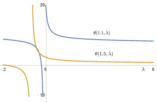
5. A Particular Example

In this section, we present a particular case where to apply the existence results given in previous section.

Example 1.

Let us consider Problem (1) with ${\lambda }_1^{*}<\lambda \le 0$, $\alpha =\frac{3}{2}$, $\mu =\frac{1}{12}$, $\eta =\frac{1}{16}$, $\lambda =-\frac{1}{2}$, $c_1=\frac{1}{3}$.

A simple calculation yields to $(1-\mu \theta -\eta \sigma )\approx 0.0998338>0$ and $c\approx 0.0160729$.

Let

$$f(t,u)=\delta \sqrt{1+t}(1+u^{\frac{3}{2}}),\mathit{for}\delta >0.$$

Let ${\rho }_1,{\rho }_2>.$ Then

$$f_{{\rho }_1}^1=min\left\{\frac{f(t,u)}{{\rho }_1}:t\in [\frac{1}{3},1],u\in [0,\frac{{\rho }_1}{c}]\right\}=\frac{2}{\sqrt{3}{\rho }_1}\delta ,$$

and

$$f^{{\rho }_2}=max\left\{\frac{f(t,u)}{{\rho }_2}:t\in [0,1],u\in [0,{\rho }_2]\right\}=\frac{\sqrt{2}({\rho }_2^{\frac{3}{2}}+1)}{{\rho }_2}\delta .$$

Moreover, it is not difficult to verify that $H\ge 0.0213044$ and $m_1\le 0.0504397$.

Hence, from Theorem 2, for any ${\rho }_1,{\rho }_2$ such that ${\rho }_1<c{\rho }_2$ and

$$\frac{\sqrt{3}{\rho }_1}{2}{m}_1<\delta <\frac{{\rho }_2}{\sqrt{2}(1+{\rho }_2^{\frac{3}{2}})}H$$

Problem (1) has at least one solution $u\in C_{1/2}\left(I\right)$, such that ${\parallel u\parallel }_{2-\alpha }\le {\rho }_2$ and there is $t_0\in [c_1,1]$ for which $t_0^{2-\alpha }u\left(t_0\right)\ge {\rho }_1$.

In particular, since the minimum on the left-hand side of previous inequality is 0 and, by defining

$$f\left(x\right)=\frac{x}{1+x^{3/2}}$$

we have that

$$\underset{x\ge 0}{max}\left\{f\right(x\left)\right\}=f\left(\sqrt[3]{4}\right)\approx 0.529134,$$

we have that Problem (1) has a non-negative and non-trivial solution for all

$$0<\delta <0.00797113,$$

such that ${\parallel u\parallel }_{1/2}\le \sqrt[3]{4}.$

References

1. Butzer, P.L.; Westphal, U. An introduction to fractional calculus. In Applications of Fractional Calculus in Physics; Hilfer, R., Ed.; World Scientific: Hackensack, NJ, USA, 2000. [Google Scholar]
2. Gorenflo, R.; Mainardi, F. Fractional calculus: Integral and differential equations of fractional order. In Fractals and Fractional Calculus in Continuum Mechanics; Carpinteri, A., Mainardi, F., Eds.; Springer: New York, NY, USA, 1997; pp. 223–276. [Google Scholar]
3. Herrmann, R. Fractional Calculus: An Introduction for Physicists, 2nd ed.; World Scientific: Singapore, 2014. [Google Scholar]
4. Miller, K.S.; Ross, B. An Introduction to the Fractional Calculus and Fractional Differential Equations; John Wiley & Sons: New York, NY, USA, 1993. [Google Scholar]
5. Povstenko, Y. Linear. In Fractional Diffusion-Wave Equation for Scientists and Engineers; Birkhäuser: New York, NY, USA, 2015. [Google Scholar]
6. Samko, S.G.; Kilbas, A.A.; Marichev, O.I. Fractional Integrals and Derivatives: Theory and Applications; Gordon and Breach: Yverdon, Switzerland, 1993. [Google Scholar]
7. Uchaikin, V.V. Fractional Derivatives for Physicists and Engineers; Springer: Berlin, Germany, 2013. [Google Scholar]
8. Ahmad, B.; Alsaedi, A.; Alghamdi, B.S. Analytic approximation of solutions of the forced Duffing equation with integral boundary conditions. Nonlinear Anal. Real World Appl. 2008, 9, 1727–1740. [Google Scholar] [CrossRef]
9. Cabada, A.; Aleksić, S.; Tomović, T.V.; Dimitrijević, S. Existence of Solutions of Nonlinear and Non-local Fractional Boundary Value Problems. Mediterr. J. Math. 2019, 16, 119. [Google Scholar] [CrossRef]
10. Chen, P.; Gao, Y. Positive solutions for a class of nonlinear fractional differential equations with nonlocal boundary value conditions. Positivity 2018, 22, 761–772. [Google Scholar] [CrossRef]
11. Graef, J.R.; Kong, L.Q.; Wang, M. Uniqueness of positive solutions of fractional boundary value problems with non-homogeneous integral boundary conditions. Fract. Calc. Appl. Anal. 2012, 15, 509–528. [Google Scholar] [CrossRef]
12. Jiang, J.; Liu, W.; Wang, H. Positive solutions to singular Dirichlet-type boundary value problems of nonlinear fractional differential equations. Adv. Differ. Equ. 2018. [Google Scholar] [CrossRef]
13. Tellab, B.; Haouam, K. Solvability of semilinear fractional differential equations with nonlocal and integral boundary conditions. Math. Eng. Sci. Aerosp. 2019, 10, 341–356. [Google Scholar]
14. Zhang, X.; Wang, L.; Sun, Q. Existence of positive solutions for a class of nonlinear fractional differential equations with integral boundary conditions and a parameter. Appl. Math. Comput. 2014, 226, 708–718. [Google Scholar] [CrossRef]
15. Ahmad, B.; Nieto, J.J. Existence results for nonlinear boundary value problems of fractional integro differential equations with integral boundary conditions. Bound. Value Probl. 2009. [Google Scholar] [CrossRef] [Green Version]
16. Benchohra, M.; Cabada, A.; Seba, D. An existence result for nonlinear fractional differential equations on Banach spaces. Bound. Value Probl. 2009. [Google Scholar] [CrossRef] [Green Version]
17. Feng, M.; Liu, X.; Feng, H. The existence of positive solution to a nonlinear fractional differential equation with integral boundary conditions. Adv. Differ. Equ. 2011. [Google Scholar] [CrossRef] [Green Version]
18. Guo, D.; Lakshmikantham, V. Nonlinear Problems in Abstract Cones; Academic Press: New York, NY, USA, 1988. [Google Scholar]
19. Zeidler, E. Nonlinear Functional Analysis and Its Applications. I. Fixed-Point Theorems; Translated from the German by Peter R. Wadsack; Springer: New York, NY, USA, 1986. [Google Scholar]
20. Amann, H. Fixed point equations and nonlinear eigenvalue problems in ordered Banach spaces. SIAM Rev. 1976, 18, 620–709. [Google Scholar] [CrossRef]
21. Cabada, A.; Infante, G.; Tojo, F.A.F. Nonzero solutions of perturbed Hammerstein integral equations with deviated arguments and applications. Topol. Methods Nonlinear Anal. 2016, 47, 265–287. [Google Scholar] [CrossRef] [Green Version]
22. Frigon, M.; Infante, G.; Jebelean, P. Fixed Point Theory and Variational Methods for Nonlinear Differential and Integral Equations; Lecture Notes in Nonlinear Analysis, 16. Juliusz Schauder Center for Nonlinear Studies, Toruń; Nicholas Copernicus University: Toruń, Poland, 2017; p. 192. [Google Scholar]
23. Infante, G.; Webb, J.R.L. Nonlinear nonlocal boundary value problems and perturbed Hammerstein integral equations. Proc. Edinb. Math. Soc. 2006, 49, 637–656. [Google Scholar] [CrossRef] [Green Version]
24. Lan, K.Q.; Webb, J.R.L. Positive solutions of semilinear differential equations with singularities. J. Differ. Equ. 1998, 148, 407–421. [Google Scholar] [CrossRef] [Green Version]
25. Webb, J.R.L. Remarks on positive solutions of three point boundary value problems. Discret. Contin. Dyn. Syst. 2003, 905–915. [Google Scholar] [CrossRef]
26. Cabada, A.; Wanassi, O.K. Existence and uniqueness of positive solutions for nonlinear fractional mixed problems. arXiv 2019, arXiv:1903.09042. [Google Scholar]
27. Kong, Y.; Chen, P. Positive solutions for periodic boundary value problem of fractional differential equation in Banach spaces. Adv. Differ. Equ. 2018. [Google Scholar] [CrossRef]
28. Lan, K.Q. Multiple positive solutions of semilinear differential equations with singularities. J. Lond. Math. Soc. 2001, 63, 690–704. [Google Scholar] [CrossRef]
29. Liang, S.; Zhang, J. Existence of multiple positive solutions for m-point fractional boundary value problems on an infinite interval. Math. Comput. Model. 2011, 54, 1334–1346. [Google Scholar] [CrossRef]
30. Cabada, A.; Hamdi, Z. Existence results for nonlinear fractional Dirichlet problems on the right side of the first eigenvalue. Georgian Math. J. 2017, 24, 41–53. [Google Scholar] [CrossRef]
31. Kilbas, A.; Srivastava, H.; Trujillo, J. Theory and Applications of Fractional Differential Equations. In North-Holland Mathematics Studies; Elsevier: Amsterdam, The Netherland, 2006; Volume 204. [Google Scholar]
32. Lloyd, N.G. Degree Theory; Cambridge University Press: Cambridge, UK; New York, NY, USA; Melbourne, Australia, 1978; Volume 73. [Google Scholar]
Figure 1. Graph of θ for α = 1.1 (blue) and α = 1.5 (orange).
Mathematics 08 00255 g001
Figure 2. Graph of σ for α = 1.1 (blue) and α = 1.5 (orange).
Mathematics 08 00255 g002