1. Introduction
In the years since the Great Recession of 2008, economists have studied which policy responses worked and which ones did not, and two findings stood out. First, fiscal policy is an important tool to fight a recession and second, it is crucial to have a quick and effective response to a recession in order to limit its longest-lasting and most-severe effects. In light of recent crises in the economy worldwide, the issue of forecasting Gross Domestic Product (GDP) is highly debated.
During the last ten years Italy suffered two great crises, in 2008 and 2011, and it is actually living a stagnation. Italian Real GDP started to decline significantly in 2008:Q2 with a short drop-in 2007:Q4, and its growth did not recover until 2009:Q4. For this, the cumulative fall from the 2008:Q1 peak until 2009:Q4 was 23.49%. In addition, Italy suffered a national debt crisis in 2011. Real GDP started again to fall in 2011:Q4 and growth was not resumed until 2013:Q4. The aggregate fall for this period was 19.34% based on the last peak in 2011:Q3. Overall, Italy from the two crises, in just ten years, lost 30.6% of the real GDP.
Policy decision-makers sometimes have to make speed choices and often found to be wrong due to the lack of knowledge on the current economy in their country. If the drop in output could be detected by policy makers, financial policies could be adjusted together with fiscal policies to avoid the recession or to limit the effects of the same on the real economy. The major statistical indicators that are publicly released offer many doubts and uncertainties for their economic forecasts as they are released with very late and are frequently subject to major revisions. The development of new predictive models is a current topic for many institutions and central banks and is an important instrument for them to help address these gaps. In fact, current methodologies often lack the ability to predict the outcome of a recession in a prompt and efficient manner. This is the case of the National Bureau of Economic Research’s methodology, as it needs two consecutive quarters with a negative growth to announce the beginning of a recession. This determines an important lag before making aware policy makers of the incoming storm. A prompt insight in this field could make the difference, allowing policy makers to issue all the necessary reforms act to overcome the situation reducing the negative effect of the recession on all economic aspects.
In such a context, the explosion of new technologies like Artificial Intelligence (AI) and different Machine Learning (ML) techniques play an important role and can be used to manage complex economic systems equipped with huge data. The use of ML models is now guaranteed to be able to manage large amounts of data and provide great guarantees in terms of accuracy of the final model even when faced with a greater number of potential regressors compared to the presence of small volumes of observations. On the other hand, ML represents a key approach to build models capable of correlating all data from different economic sources and dynamically responding to different problems, without the help of human beings.
The purpose of our analysis is to adopt and test a forecasting model for GDP movements, using several advanced ML techniques. We examine whether ML algorithms can improve forecasting accuracy and try to define which variables drive the economy recovery and forecast recession. We started by an overview of various theoretical macro-economic models. There is a relevant debate about which variables can give insight on the state of economic health. In literature, there are many indicators built for this purpose as it will be shown in the upcoming pages. With the advent of new technologies, there has been a considerable increase in accuracy regarding forecasts on financial market trends. This automation has allowed the introduction of ad-hoc algorithms able to analyse, in a short time, a considerable amount of data with the aim of performing accurate forecasts by improving the robustness of these systems. For this reason, the authors propose a technique based on non-linear autoregressive Levenberg-Marquardt (LM) algorithm [
1] that, starting from the analysis of historical data, is able to perform an accurate prediction of future values of the GDP. We test our model on short-term forecasts of real GDP growth in Italy, by comparing the forecasts obtained from these models with the real value of the GDP by evaluating the ML performance compared to the classical statistical approaches. We used data analytics with only the default input parameters to the LM algorithm, by making the robustness check in applying different settings by using Matlab software packages.
The present paper is structured as follows: in
Section 2 we describe briefly the literature on GDP movements in Italy.
Section 3 illustrates the dataset that we have chosen to carry out the study and the motivation that led us to the use of these variables.
Section 4 describes the chosen methodologies.
Section 5 discusses performance evaluation results for the proposed model. Finally,
Section 6 summarizes the conclusions and discusses future research directions.
2. Related Literature
There are many theories about how economy works, and which variables must be analysed so to keep prompt insight on economic trends. In literature it is debated how to conduct forecasting research in macroeconomics field and scholars fundamentally divide in two main clusters, based on the adopted research methodology. In the study conduct by Nyman and Ormerod [
2], which we take as the main example on the methodology adopted in our case study, they focus on short-term forecast of real GDP growt for United States and United Kingdom both with a statistical approach by using Ordinary Least Squares (OLS) regression and Random Forest (RF) ML technique by demonstrating how the latter guarantee more accuracy, especially in the great recession of 2008/09. A main group adopts a statistical approach, assuming that data can be explained by stochastic models and others have a more mechanical approach, based on the exploitation of algorithms and treating data as instruments to understand unknown mechanisms [
3]. Other works in the recent literature witnesses the widespread of approaches less common, such as the Kinetic Theory for Active Particles (KTAP) approach to the modelling of economic systems [
4,
5]. The authors of Reference [
6] propose a model of credit risk infection on the performance of financial networks through the inclusion of infected elements, distinguishing systemic risk from idiosyncratic risk and testing it in different topological networks with different levels of connectivity. Economics journals are reluctant about accepting research without the adoption of methods with formal properties—including large sample properties of estimators and test (regarding consistency, normality and efficiency. However, the increasing in knowledge in supervised and unsupervised ML techniques are undeniable, just seeing the application of this technology in pattern, voice or photos recognition, but also relevant in recent literature in the field of economics, econometrics and statistics [
7]. The authors of Reference [
8], for instance, use ML in econometric field and the idea is that ML is able to discover complex structure in the data and the intuitions is that this new frontier in econometrics can provide tools to overcome the limits in forecasting prediction, in particular in GDP growth. They support their insight with several ML techniques applied on prediction of house values by using RF and Ensemble algorithms by showing a double accuracy capacity than traditional econometric techniques such as OLS regression. In this contribution [
9] you develop a predictive methodology of a Lyapunov-based economic model predictive control (LEMPC) in the field of economic optimization by demonstrating its economic optimality and closed-loop stability through an ensemble of Recurrent Neural Networks (RNN) and an k-fold cross-validation applied in nonlinear systems.
Other manuscripts [
10,
11] use the same Lyapunov-based approach, respectively, to solve the problem of predictive control model (MPC) design of the data-based economic on a non-linear chemical process system and to address the problem of control system design for chemical processes to guarantee economic optimization and process operational security in stochastic nonlinear systems.
Another work [
12] demonstrated, through the use of the Bayesian Additive Regression Tree (BART) model, that predictions using a high number of predictors offer more accuracy in short macroeconomic time series. The authors of Reference [
13] present a Nonlinear autoregressive (NAR) approach of neural network for the prediction of time series based on the LM method, used for management of network parameters, and introducing a heuristic law that regulates the learning process and modifies the topology of the network. The simulation phase of the prediction has been applied through the Monte Carlo method also with the insertion of a Gaussian noise. Another study [
14] compared the short-term forecasting capabilities of different statistical approaches using a dataset with multiple monthly indicators embedded with little but very valuable information, showing that this forecasting strategy is better than those based on a single indicator. This study includes Europe and the five largest countries in the 1996-2011 period.
The authors of Reference [
15], using an ARIMA (Auto-Regressive-Integrated-Moving-Average) model to predict future time series through the Box - Jenkins technique, accentuate the importance of GDP as one of the most important indicators for an economic growth of a country and consider that the correct prediction of this indicator is fundamental in central bank decision-making for all countries.
Even thought there is not a clear evidence about how ML can increase forecasting accuracy in the predictions obtained, in literature there are many examples on how forecasting accuracy could be augmented by this technology. However, there is an evidence that simple univariate linear models are often more robust than multivariate [
16].
The main contribution that we present in this paper is that ML algorithms, such as the LM algorithm, offer better performance in forecasting the economic recession than the classic statistical approaches commonly used. Another important contribution is that using only the raw explanatory variables without modifications, we obtain good results by demonstrating how, from LM approach, it is possible to correctly evaluate the state of health of the country Italy, taking all the necessary precautions from a political point of view.
3. Dataset
In this section, we provide details about the Italian economic dataset by introducing the main indicators of credit and real economic activity. We conduct the research using Italian economics data, available from several sources. Based on a research conducted by Fildes and Stekler [
17], that asserts there is no real method that demonstrates that the accuracy of one model is better than another or that it is better during the time, we decided to take data spanning from the period 1995:Q1 to 2019:Q2 (data are available in ISTAT database), and we consider as dependent variable the adjusted quarterly Italian GDP. This represents the amount of the production made in Italy in each quarter without adjustment for seasonality and inflation. We decided to choose this variable in order to maintain in our model all the information and all the effects due to other economic variables. From the adjusted GDP growth rate, policy maker is able to evaluate the effectiveness of their policy and to introduce new measures. It should be highlighted that the dataset taken into consideration has been constructed based on our theoretical knowledge and without any pre-assessment of how the variables were chosen are correlated with GDP growth. For the design of the dataset, we used variables from several official sources by specifying for each figure the source in the caption section.
Once we defined the problem and built the dataset, we did not do any statistical survey or feature engineering work to try to extract important characteristics from the raw data and thus improve the performance of ML algorithms on macroeconomic time-series predictions. We considered the following Italian economics variables as explanatory variables (at the same period previously indicated): Inflation rate, Unemployment rate, Industrial production, Gross debt, FTSE Mib, Average interest rate at issuing for BOT 3-6-12 month, Interest rate at issuing for BTP 10 years, Balance of payments, Final consumption aggregates, State budget and Government deficit/surplus.
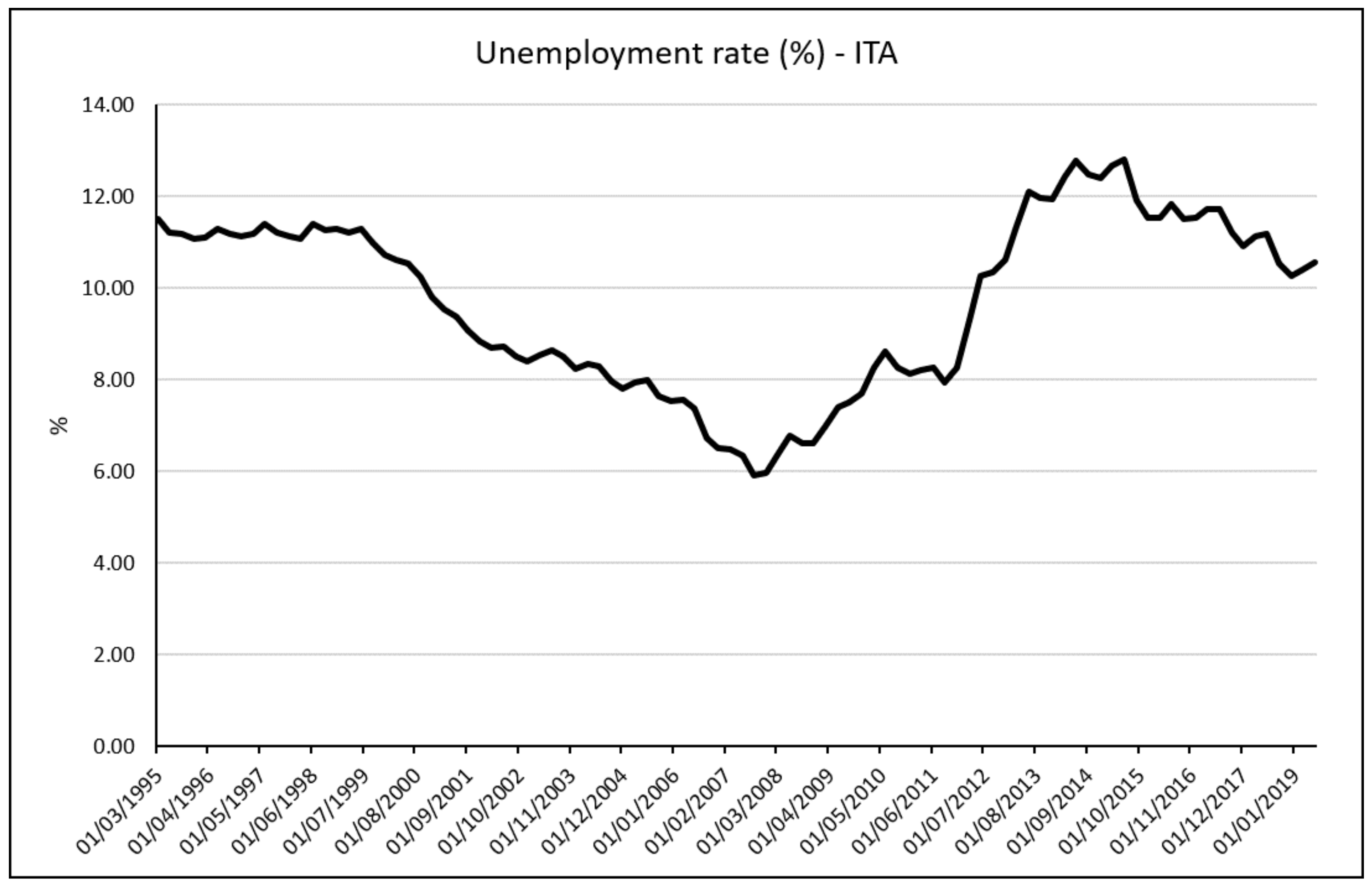
3.1. Unemployment Rate
Unemployment rate is an important indicator used to determine the health of the economy condition of a country. Indeed, it expresses the well-being of the labour market. It is simply calculated by dividing the number of unemployed people by the number of the civilian labour force. In order to be counted in the unemployment rate, the person must be without a job but active to look for a new one. For this reason, there is an important gap between the statistics about the unemployment rate, and the real unemployment rate, which is higher because it includes those who are discouraged and ceased looking for a job.
If we look at
Figure 1, unemployment rate is almost stable in the long run and it is, on average, below 10%. If we consider the pure values of the indicator, unemployment rate is a lagging indicator to forecast GDP. This means that it measures the effect of economic events, such as a recession: this because it does not rise significantly until after a recession has already started and it will continue to rise even after the economy has started to recover. This happens for several reasons, one is that employers are reluctant both to lay people off when the economy turns bad and to hire new workers until they are sure the economy is well into the expansion phase of the business cycle. The decreasing of the unemployment rate is usually taken as an important positive indicator of the state of things. It means that employers’ demand works to increase the supply of their products and services in a growing market and at the same time workers can have new means to sustain their own demand.
The decreasing of the unemployment rate is a positive indicator that could change its value until it reaches the condition of full employment. It is not the case of the Italian economy but of the United States. As said above, US are living the longest growth turn of a business cycle from the Great Recession in 1929 and after 10 years from the Great Recession in 2008, it records an unemployment rate of 3.5%. A condition of full employment should be considered as a premonitory of a future recession because it denotes the achievement of the state of the economy maturity. In recent work, it was demonstrated that when an economy reaches an unemployment rate below what considered as the nature rate of unemployment, it implies that the only way forward is an increase in unemployment and this is linked with crises [
18]. We do not consider Italian economy as a full employed economy. The reason we consider unemployment rate is variation in the short period. We agree with Reference [
19], which created a Recession Indicator that confronts the real unemployment rate with its lowest point in the last year, taking a quarterly average a rapid increase, although relatively modest, in the unemployment rate was a clear indication that a recession is underway. If the current level is higher than 0.3 based points there is a concrete risk of crises that become reality if it exceeds 0.5 based points.
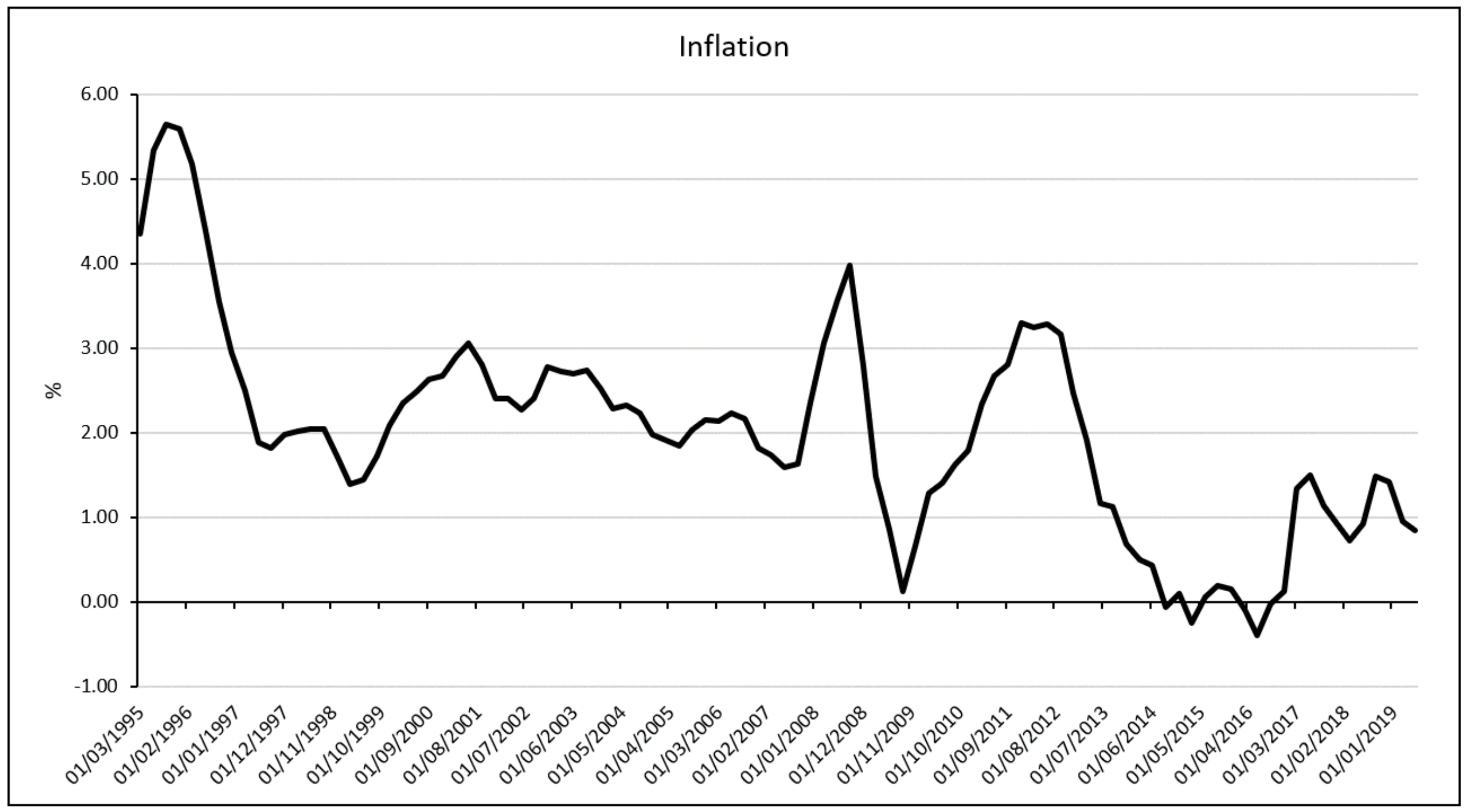
3.2. Inflation
We decided to include inflation as an explanatory variable of the economic contest. In macroeconomics, inflation represents an indicator for which the average price of goods and services increases over a given period. Relationship between inflation and economic growth is relevant for central banks and governments because it generates effects in the purchasing power of a nation’s currency. The first works about the importance of inflation in the economy field were established thanks to the works of monetarists. According to Reference [
20], it is inferred that central bank policy should perform a primary role in monetary policy to the benefit of economic growth. Orphanides and Solow [
21] analyzed the effect of money supply on the most important macroeconomic indicators showing that there is a strong correlation between inflation and GDP performance, and in 2017 an empirical confirmation was established that money and price growth has a significant impact on economic growth [
22]. High and volatile inflation undermines the confidence of foreign investors about the future course of monetary policy. Inflation also affects the accumulation of other determinants of growth such as human capital or investment in R&D: this channel of influence constitutes what is known as the accumulation or investment effect of inflation on growth [
23]. Furthermore, other studies conducted by the authors of Reference [
24] have shown that high inflation is caused by increased public spending and is the same that prevents investment and reduces productivity also in the future [
25,
26]. Other studies [
27] have shown that inappropriate and exaggerated government spending can lead to increased consumer demand and halt production investment.
Most economists today agree that there is a correlation between inflation and the macroeconomic phenomena of economic growth in a non-linear way. It is diffusely accepted the need to keep stable the inflation in order to allow investors and all the stakeholder to plan their chosen. It is a key action for the central banks to stabilise inflation rate and for several reasons, this is often targeted on 2%. Even though the action of the central bank, we see in the Italian economy important movements during all the periods under research.
As shown in
Figure 2, inflation suddenly increases over the inflation rate target and immediately after dropping closes 0%.
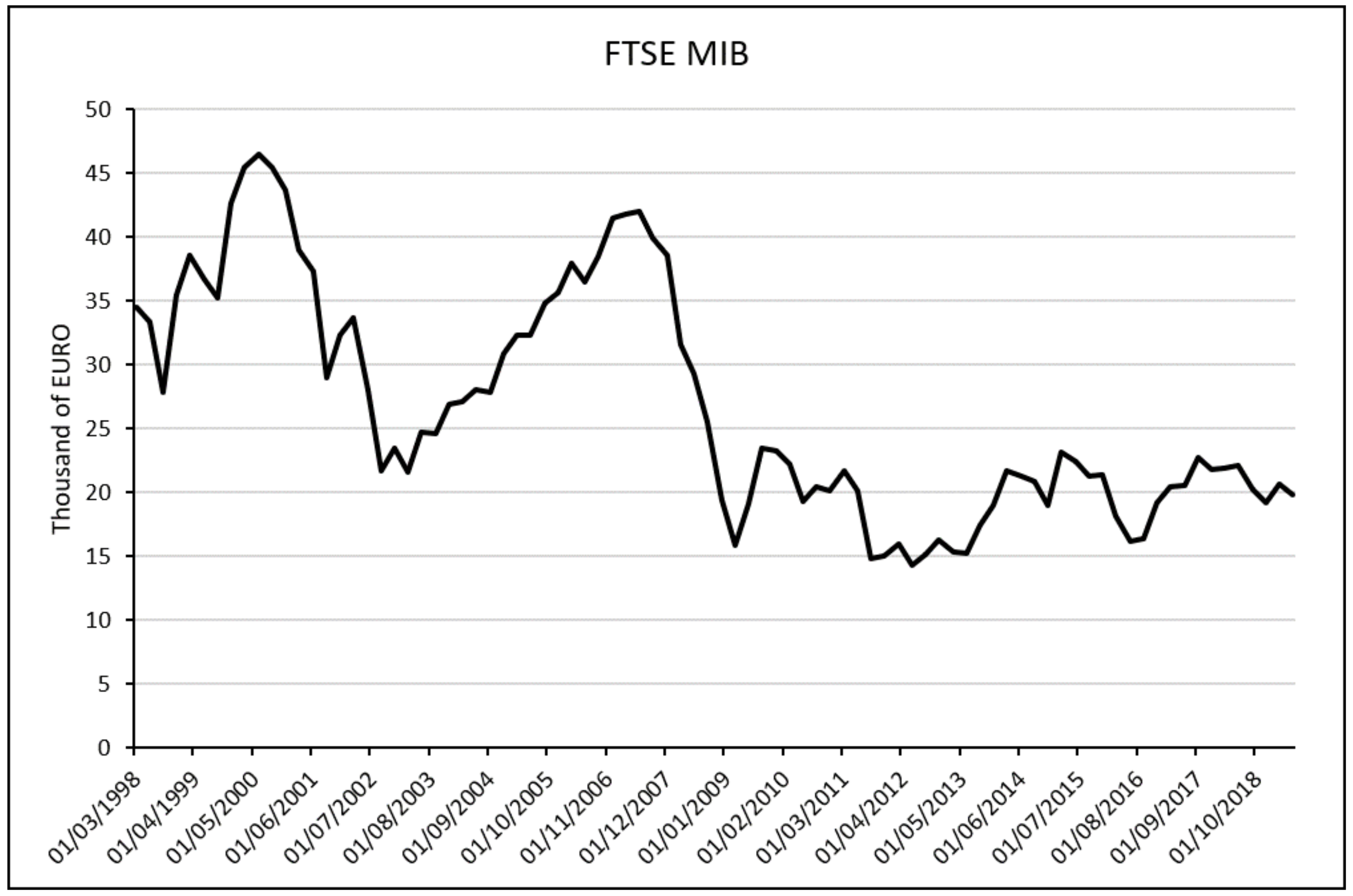
3.3. Stock Market
To conduct our research, we considered the impact of the Stock Market on the GDP. Theoretically, stock price dynamics should match real GDP movements. According to several researchers, the profitability of firms is subject to the trend of the economy. Indeed, economic growth has positive effects on Earnings per Share, dividends and stock prices [
18,
28,
29]. Furthermore, financial system may bear business cycle expansion phase [
30], contributing to the achievement of macroeconomic stability through the action of interest rates [
31]. Moreover, economic growth may increase the demand for financial services, contributing to the development of the financial system [
32]. However, these considerations are valid only in theory if only considering closed economies. In the first instance, financial markets influence the performance of the GDP by influencing economic conditions—on the one hand—and consumers’ sentiments. A widespread lack of optimism among consumer institutions and financial operators is observable when stock exchanges are in the bull phase. Indeed, in such conditions highly capitalized companies have the possibility of obtaining financing—in capital account or in debt—at low prices, allowing to expand their turnover, increase investments and hire additional workers. Investments, hires and new operations support economic growth. The widespread optimism determines a positive spiral that expresses in increased spending and earnings for corporations. On the contrary, when the stock market is in bear mode, it creates a pessimistic climate that impacts on companies, which are forced to cut costs and workers. Consumers are less likely to increase the demand of goods and services, preferring holding liquidity rather than making investments or purchasing choices. These aspects have a negative effect on GDP. The stock market should be considered a lagging indicator. Indeed, there is a significant spill over interplay between economic growth and the stock market. It has been empirically observed that after a financial shock it is normally the prelude to a period of recession [
33]. This was the case, for example, with the internet bubble crisis in the early 2000s and the south-prime mortgage crisis in 2008.
To conduct our analysis on Italian GDP movement we take under consideration the FTSE MIB (as shown in
Figure 3), which is the main Italian equity index representing approximately 80% of the Italian capitalization. It is calculated considering the 40 most capitalized Italian companies trying to give a reliable picture of the health of the various production sectors. It is calculated by measuring the performance of 40 Italian equities and it seeks to replicate the broad sector weights of the Italian stock market.
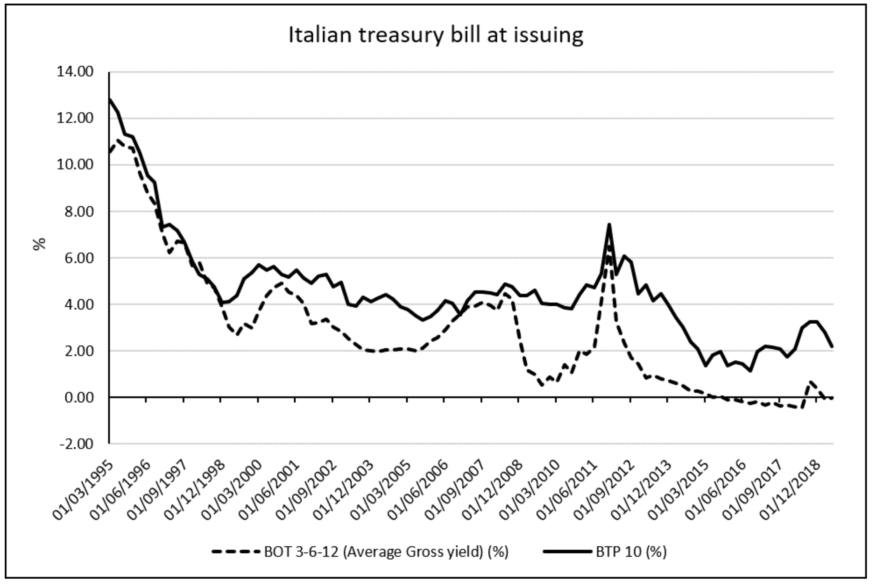
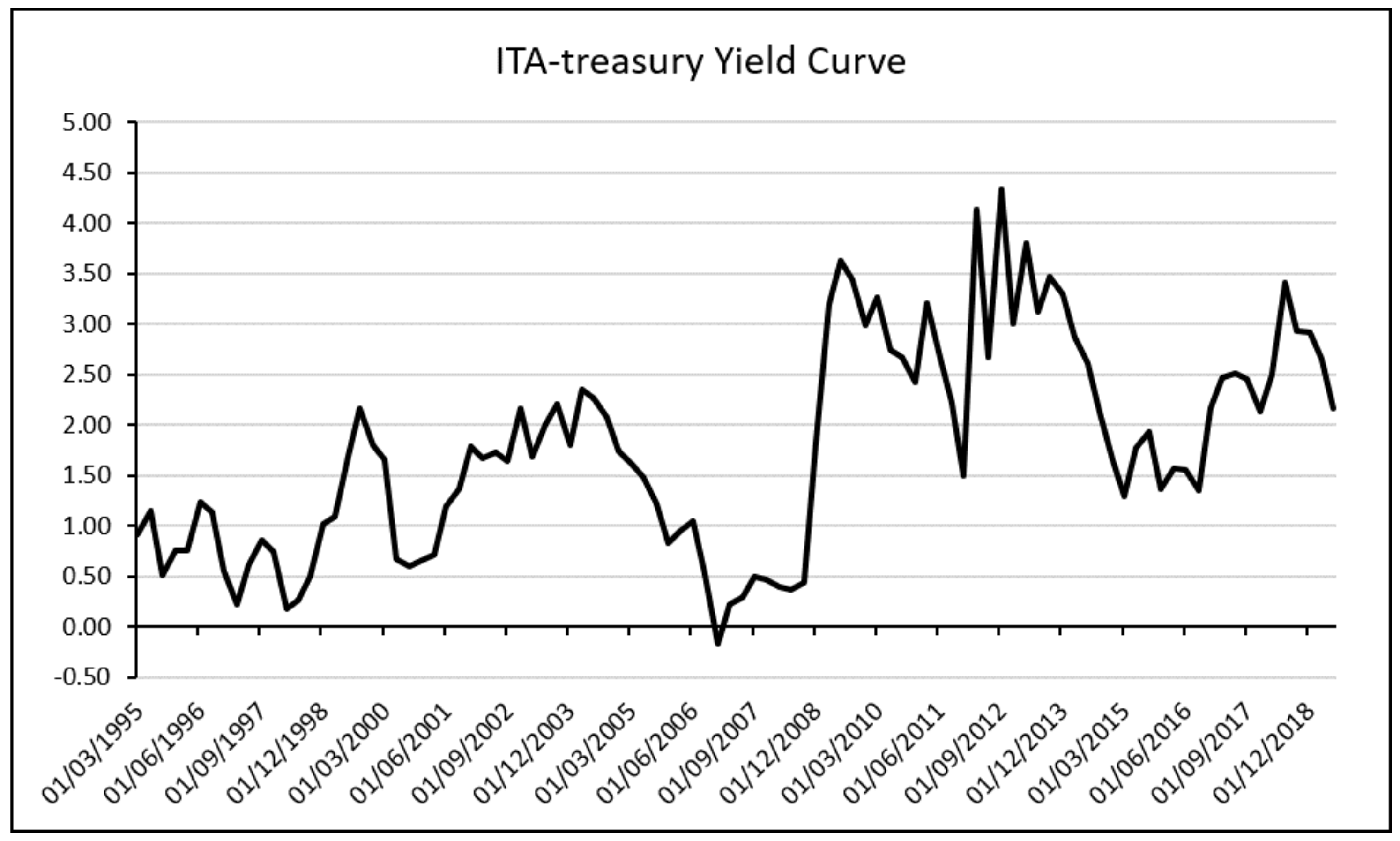
3.4. Yield Curve
The Yield Curve is the monthly average spread between the interest rate on short- term (usually considered 2 years or 3 months maturity bill) and the long-term (normally ten-year constant maturity rate) government bonds. It is an important economic indicator that measures investor confidence. Normally, investors ask for a return proportional related to the duration. In the bearish period, they are inclined to accept much lower returns for securities deemed to be safer. When this happens—the long-term interest rate falls under short-term interest rate—the yield curve is said to be inverted (negative slope). In literature, many researchers discovered important correlations between this event and the beginning of a crisis, and many are confident this is a good predictor of future economic activity [
34]. The Yield Curve tends to flatten when there is a rise in the short rate or a real growth slowdown in the near term. Furthermore, the Yield curve calculates the difference between long-term interest rate—normally and in this case study the ten years treasury bond—and short-term interest rate—normally and in this case study the three months treasury bond. They are quoted on the basis of investors’ presumptions in terms of expected inflation and expected return, which are two powerful indicators of future economic activity forecasts [
35,
36].
The Italian monthly average spread between the ten-year constant maturity rate and the three-month bond rate has turned negative before the great recession of 2008, has estimated by Estrella for the US economy. Yield Curve “inversion” is not a sufficient predictor of a future recession in light of the actual economy condition and the effects on bond market of the Quantitative Easing program that put under control the National debt crises in 2011.
Figure 4 shows the plotting of the Italian treasury bill at issuing for the period from 1995:Q1 to 2019:Q2. In particular, the dotted line represents the average interest rate at issuing request by investors for short term treasury bill maturity and the full line represents the interest rate request by investors at issuing for treasury bill at 10 years maturity.
Figure 5 shows the Yield Curve obtained by the difference between long-term and short-term treasury bill maturity for the period of 1995:Q1 to 2019:Q2.
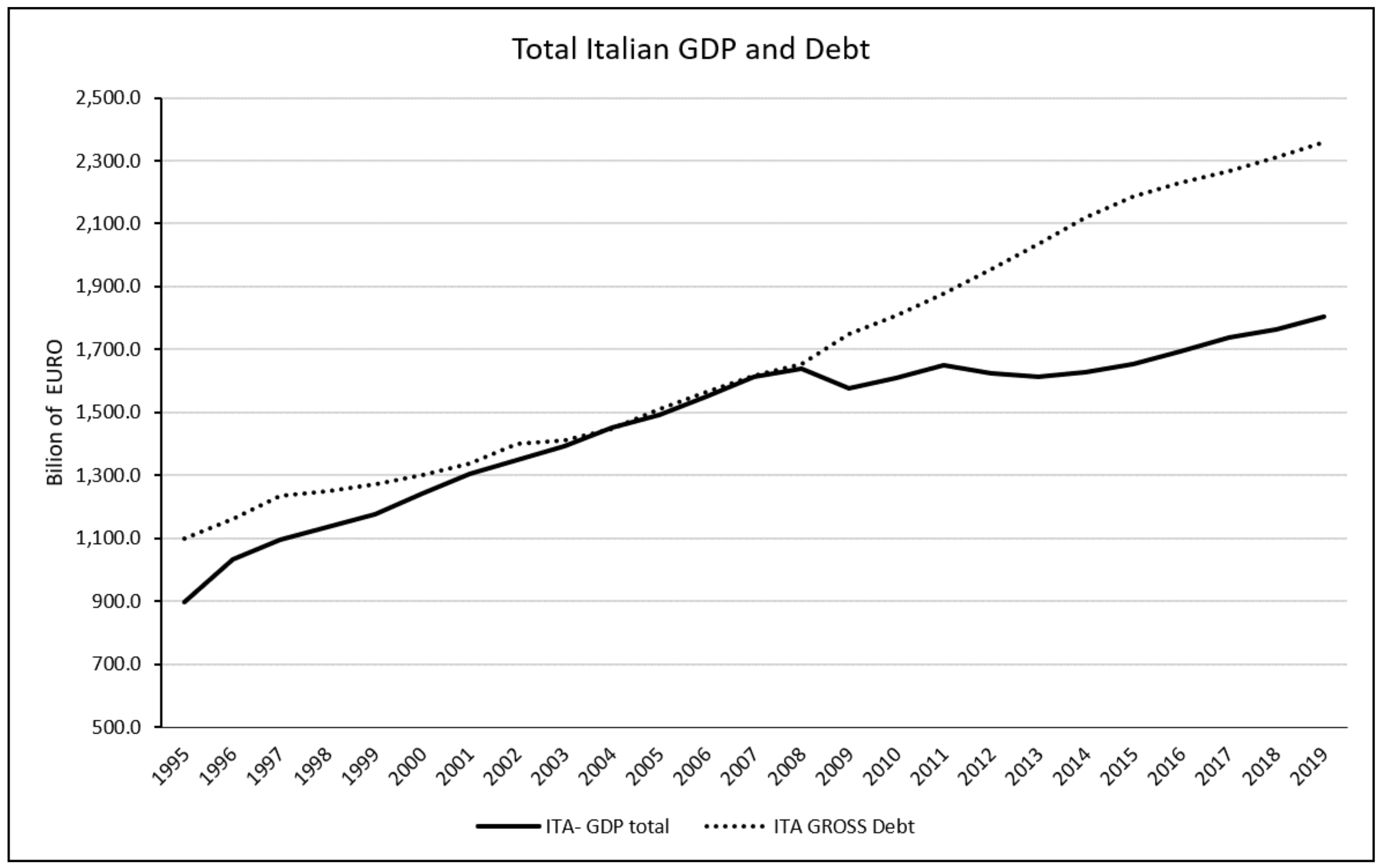
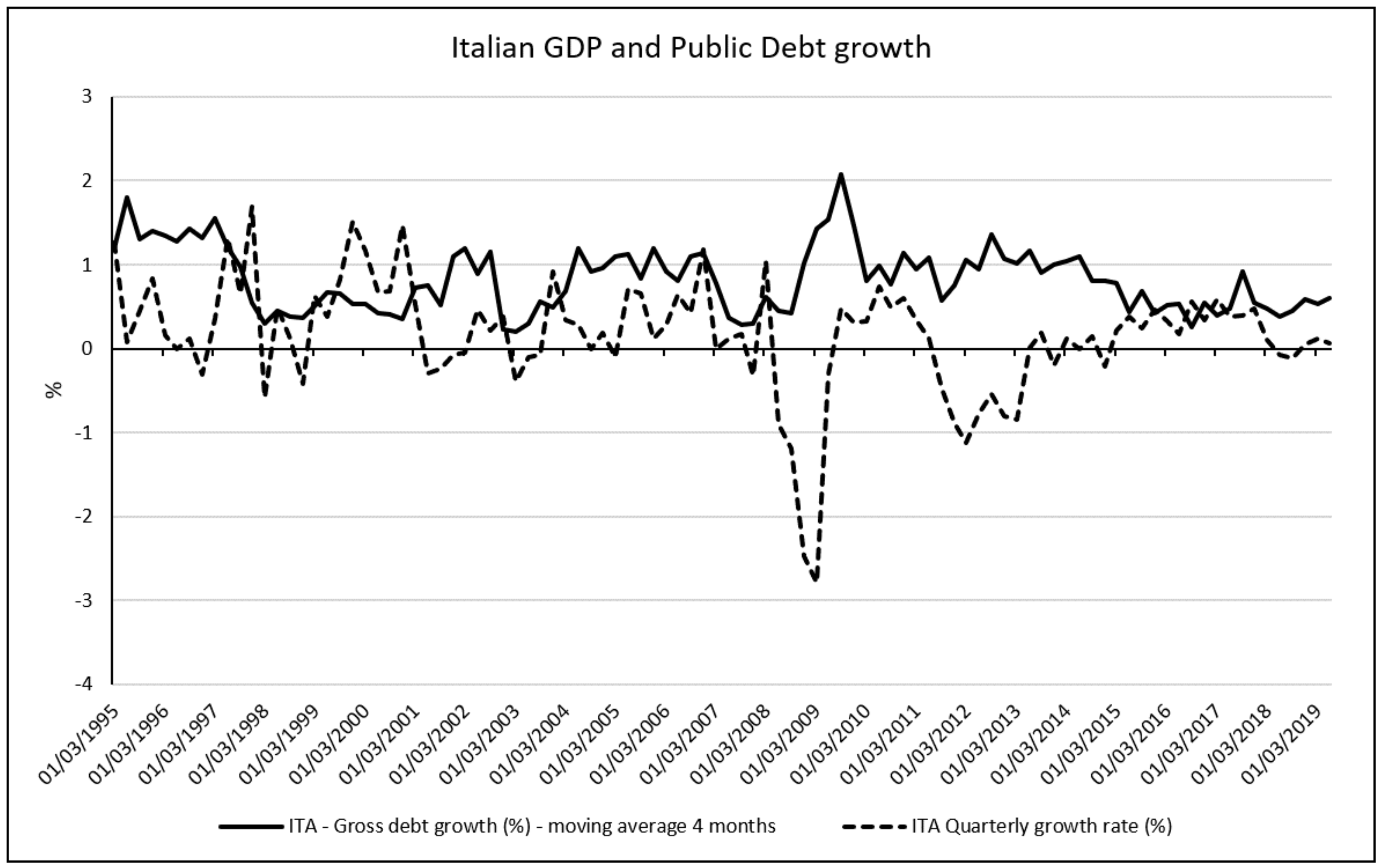
3.5. Gross Debt
In the preliminary stage of building our forecasting model, we decided to consider the Gross Debt. Gross Debt is the total liabilities owned by a country. We considered three aspects of government debt: total stock (in amount and in relation with debt-to- GDP ratio), debt growth rate and interest paid on the stock of debt. Debt dynamics and its sustainability are essential elements for the stability and future growth of an economic system. They are due to several factors and the European Central Bank (EBC) considers as a key indicator of sustainability the difference between the average interest rate paid by the government to honour the debt and the average nominal GDP growth. If the average interest paid for the debt is higher than the growth rate, it would be appropriate to intervene on general taxes in order to reduce the debt-to-GDP ratio so as to reduce the risks of future insolvency. These actions must be proportionate to the size of the debt - in absolute value - and in relation to the debt-to-GDP ratio. On the opposite, it may have no fiscal cost.
In literature, there is an ongoing debate on the effect of Debt on GDP and whether there is a hedge level of debt above which it is considered unsustainable. In literature, per se debt is not a key-driven factor of recession or reducing GDP growth in short-term, but it may reduce long-run economic growth [
37]. Other researchers argue that public debt could have a major negative effect on economic growth if it determined a reduction in productivity of public expenditures [
38], increases uncertainty or creates expectations of future financial repression [
39], and increases sovereign risk [
40], leading to higher real interest rates and lower private investment [
41,
42].
The effect of debt may depend on how it has been accumulated (for instance for investment or social expenditure), on its type and structure. Moreover, the holding of a considerable portion of public debt (in percentage) by foreign investors, in the long run, would result in an outflow of resources from the country, leading to a reduction of resources useful for supporting investments and growth. According to kinds of research, there is empirical evidence of high levels of public debt may reduce future potential growth [
37]. This can also happen for those solvent governments that decide to put in place restrictive fiscal policies aimed at containing possible sudden changes in investors’ sentiments that could cause a negative impact on future economic growth. This policy is able to strongly reduce GDP growth especially if they are put in place during a recession [
43,
44]. Precisely in these conditions, the debt, which has supported economic growth, becomes a ballast for future generations. In Italy, the situation creates concerns at several levels. In the era after the great recession, all countries are living the experience of negative interest and negative interest rate-growth differential (i-g), Italy is the only exception in all euro area (also forecast for 2020) [
45].
In the
Figure 6 and
Figure 7, we show how it is clear that after the great recession in 2008, the Italian government began to produce constantly a primary fiscal deficit at a higher rate than GDP growth rate.
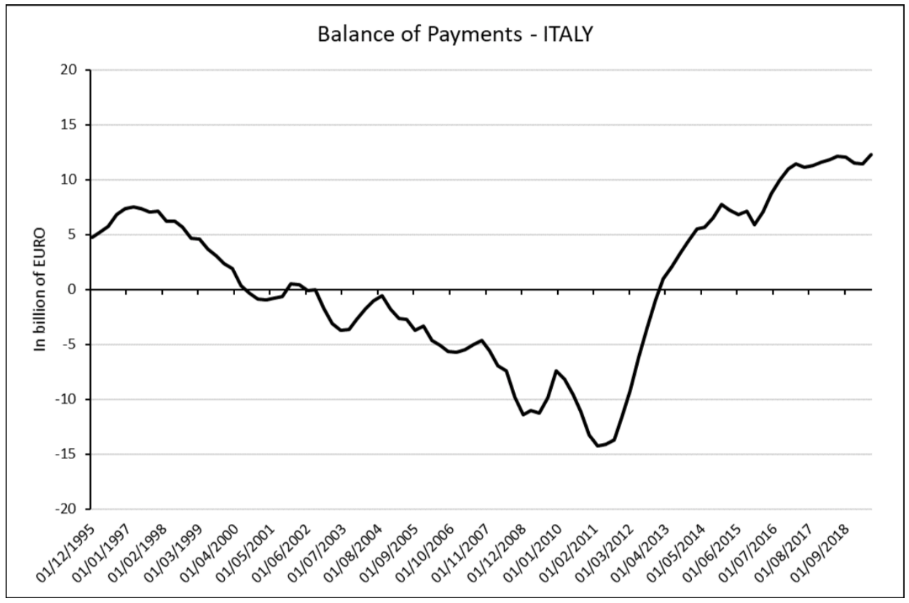
3.6. Balance of Payment
The balance of payments (BoPs) is the measure of trade in goods, services, investment incomes and net transfers with foreign economies. A negative value means that the foreign countries demand of goods produced by a country is lower than the demand of foreign good by that country. Large current account deficit is considered a potential macroeconomic problem because a flow of wealth comes out from a country. During the expansionary phases of the economic cycle, there is a significant increase in consumer spending. This increase in demand for goods and services, if not supported by a development of the economic system, determines an impressive outflow of resources towards other national economies which in the long run can undermine investments in physical and intellectual capital (in the short term) and the growth of the country system (in the long run). This phenomenon depends on the growth drivers that support economic growth. If the key factors of economic growth are given by investments in physical and intellectual capital and by foreign demand, then economic growth can be consistent with a current account surplus. If in the expansionary phase of the economic cycle, the savings rate of households and the growth rate of investments is stable, the trend of the trade balance will be stable with consequent growth and accumulation of resources for the economy in question. However, if growth is sustained by consumption satisfied by foreign goods and services at the expense of internal savings and investments, it translates into a downturn of the balance of payment, which if prolonged over time can undermine the possibility of future growth irremediably. That’s what happened in Italy since 1999. Italian economy grew for all the period until the great recession in 2008. The total expenditure (both private and public) rose and the investment and industrial production remained on average constant. This behaviour brought the Italian economy in a weaker situation. Since 2013 the BoPs curve inverted in a positive region. That’s not happening by virtue of foreign demand and industrial production but as a consequence of change the behaviour of public and private after the two crises that Italy met. In
Figure 8 we show the plotting of the Italian BoPs for the period from 1995:Q1 to 2019:Q2.
4. Methods of Analysis
In this section, we examine the analysis methodology used and provide an overview of the models taken into account for both the statistical and ML approaches. We use an ML supervised approach, with a labelled dataset. Training data are mapped to the new values by the input data (macroeconomic values) and produce the output (GDP values). This method is fast and usually produces accurate results. We use a multivariate regression analysis method to identify the relationship between the variables. ML architectures play an important role in the economic data and can be used in order to fit very complex non-linear systems with a large amount of data by improving short-term forecasting accuracy and predicting periods of recessions. At the first stage, we have conducted descriptive and correlation analysis to understand the nature and the behaviour of the variable chosen on a theoretical basis. Then, we perform the robustness check as a structural validation test, thus verifying how estimates of the initial regression coefficient perform when the regression term is modified with inserting or expelling regressors. Then, we compared the results by using seven regression estimation techniques:
Autoregressive (AR) model;
Ordinary Least Squares regression (OLS);
Nonlinear Autoregression models (NAR);
Nonlinear Autoregressive with exogenous variables model (NARX);
Support Vector Regression (SVR);
K-Nearest Neighbors (KNN);
Boosted Trees (BT).
AR model (
1) is usually used in the economic field to describe stochastic processes that vary over time. This model implies that the output variable depends linearly on its previous values and a stochastic term, thus using the observations of the previous time steps as input values to predict the value at the next step. We used the AR model as a benchmark for quarterly GDP growth.
where
c is a costant,
are parameters,
are the past time-series values, and
is random noise.
OLS is one of the most used methods for estimating the parameter of a linear regression model. This methodology chooses the parameter of the linear function in order to minimize the sum of squares of errors, that is the difference between prediction and reality. For the regression goal we used all the features to predict the output. However, to understand if this is a non-linear problem, just run the fit function on the sampled data and you will get a high error.
NARX model is a nonlinear autoregressive model (NAR) with exogenous inputs values, so, it takes into account the current value of a time series with both the past values of the same series and the current and past values of the exogenous variable. NAR and NARX with exogenous variables models were estimated using the LM algorithm [
1]. LM (
2) was originated to solve nonlinear least-squares problems and uses the gradient descent method and the Gauss-Newton method to minimize the errors. For little sized problems, the Gauss-Newton method is better and converges much faster than gradient-descent methods. However, LM method is very similar to the gradient-descent method when the parameters are far from their optimal value. Pratically, LM adaptively modifies parameter updates between gradient descent and Gauss-Newton update [
1].
where
is a normal equation for the Gauss-Newton update, and
represents the
that is usually initialized to a large value to allow you to move in small steps in the direction of the steepest gradient descent. The advantages of implementing LM techniques is that there are two possible options for the algorithm’s direction at each iteration and also is more robust than the Gauss-Newton techniques [
46].
KNN (
3) is another approach taken for the comparison of regression models. It represents a non-parametric method based on the closest neighbours and is used in cases where the data output is a continuous rather than discrete value.
where
is the neighbour of
x with the
k closest points
.
The output is calculated based on the average of the values of its neighbours in the training set and a distance function (‘’ in our case) is used to quantify the similarity between the training and testing set. So, the prediction is based on the average of the most similar k instances and the training phase is made up of the k closest neighbours of each query point.
We used Adaptive Boosting (AdaBoost) that is an ensemble ML technique that is used in conjunction with other algorithms to improve the performance of the final model for classification rather than regression problems. The basic concept is to build a predictive model from the residuals of weak predictive models (in our case decision trees), so the final improved output will correspond to the weighted sum of the outputs of other learning algorithms called `weak learners’. The AdaBoost technique splits the space of the predictors into a set of potential values of , where corresponds to the set of characteristics of training instances n. It is an iterative algorithm that starts with the forecast of the original dataset and gives equal importance to each observation n. If the accuracy of prediction is not good using the first weak learner model, then it gives more weight to the observation that was predicted incorrectly. This procedure continues until reaching a certain setted threshold in terms of accuracy or number of weak learners.
We also used non-linear SVR that are a popular nonparametric ML methods for regression analysis that is based on kernel functions. SVR uses the same methods like Support Vector Machines (SVM) for the classification problems with a few differences. In fact, considering that the output is a real number, it is very difficult to predict the information, which has infinity possibility values. For regression problem, we set a margin of tolerance (named “epsilon”) in approximation to the SVM which would have already requested from the problem.
The nonlinear SVR function (
4) is used to predict new values:
where (
) represent the difference between two Lagrange multipliers of support vectors,
G named
is an n-by-n matrix that contains elements
and
b is the bias. To minimize errors, it determines the hyperplane which maximizes the margin, so the functions, of kernel type, transform the data into a space to high dimension, allowing learning better of nonlinear models [
47].
For the performance evaluation of the models, we use the adjusted as index of accuracy of the model used. It measures the fraction of the variance of the dependent variable expressed by the predictors. We used the Mean Square Error () as estimator that measures the average of the squares of the errors, that is, the average squared difference between the estimated values and the actual values. We train each model on a time window from 1995:Q1 to 2019:Q2 by choosing the default parameter settings for each algorithm. Next, we measure the accuracy of the predictions of each model by computing and , comparing the predictions graphically.
However, we considered that the
, alone, does not represent an always valid comparison tool since it is not possible to conclude that a model with the highest determination index is the best and we used a statistical test as further proof of the predictive superiority of the ML models. In particular, we used the Diebold-Mariano (DM) [
48] statistic test as a tool for the analysis and comparison of various forecasting models. DM test fits into the economic context by trying to establish which, between two alternative models, has the best forecasting performance of a historical time series. DM test measures the statistical significance by comparing the averages of the two loss functions (in our case, we considered MSE) by verifying the existence of the null hypothesis, thus demonstrating that the two models provide the same accuracy in the forecasts.
Although the performance of modern ML methods depends heavily on their hyperparametric configurations, we have chosen to use a default configuration for each model as these default values are usually chosen ad hoc to work well enough on a wide variety of data sets. We demonstrate the effectiveness and efficiency of this principle approach that has improved model performance without adding additional algorithmic complexity and calculation costs to the training procedure.
In
Table 1 we present the experimental environment settings in which we operate and the tools we use. We train the ML on a MacBook Pro with i7 Processor under the MacOS operating system (Mojave release), as development environment we used MATLAB software.
5. Results
In this section, we show the results obtained in terms of best fit obtained with the methodology and analysis of the regression models evaluated in
Section 4. The results indicate with a great majority that ML models are able to give better predictions in the recession periods than statistical models, obtaining a higher degree of
and a lower
than the AR statistical approach.
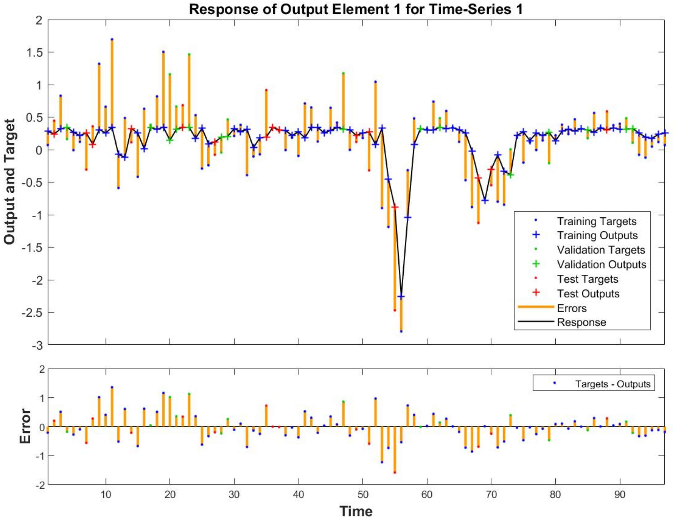
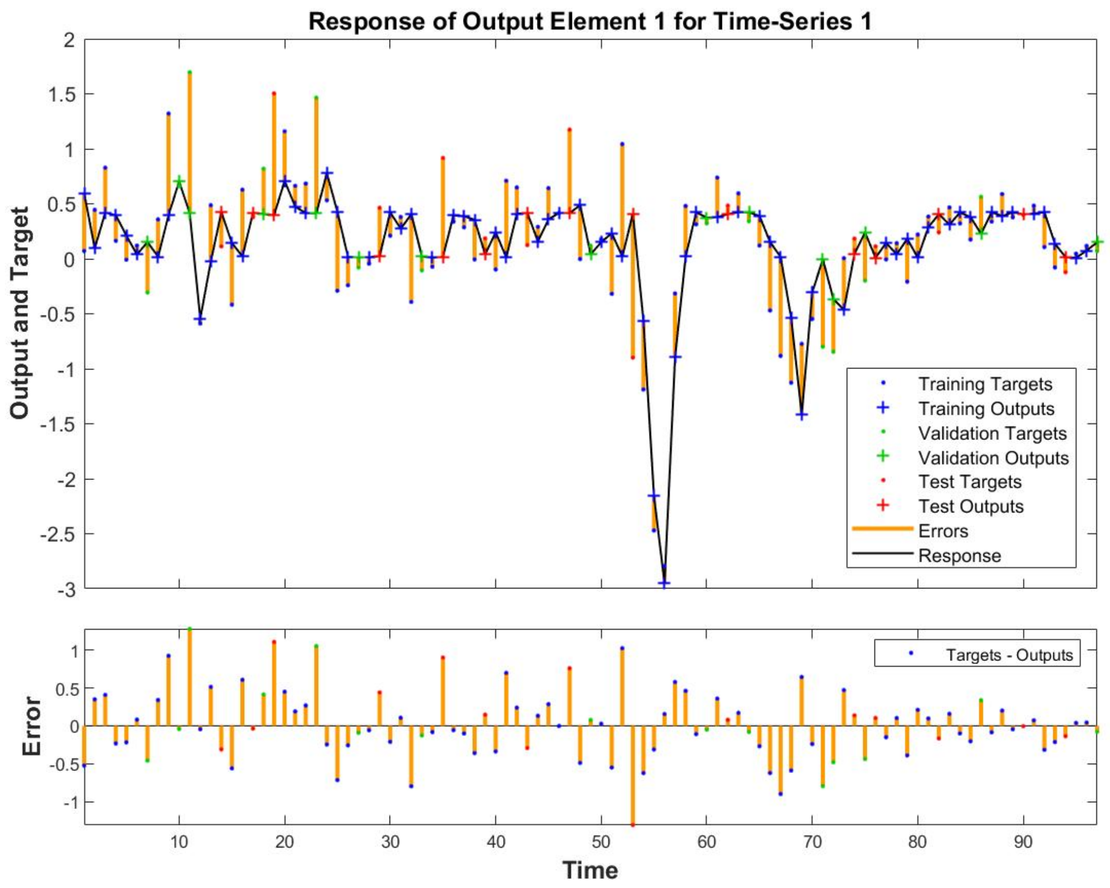
Over the period under research, all models implemented were able to forecast the two main crisis. But all of them miss a momentous negative turning (just one quarter). The most powerful model that we implemented appears to be the NARX one.
The ML algorithm that generates the autoregressive model using the exogenous variables gives surprising results. Indeed, it was able not just to obtain the lowest error (see
Figure 9 and
Figure 10), but also, as shown in
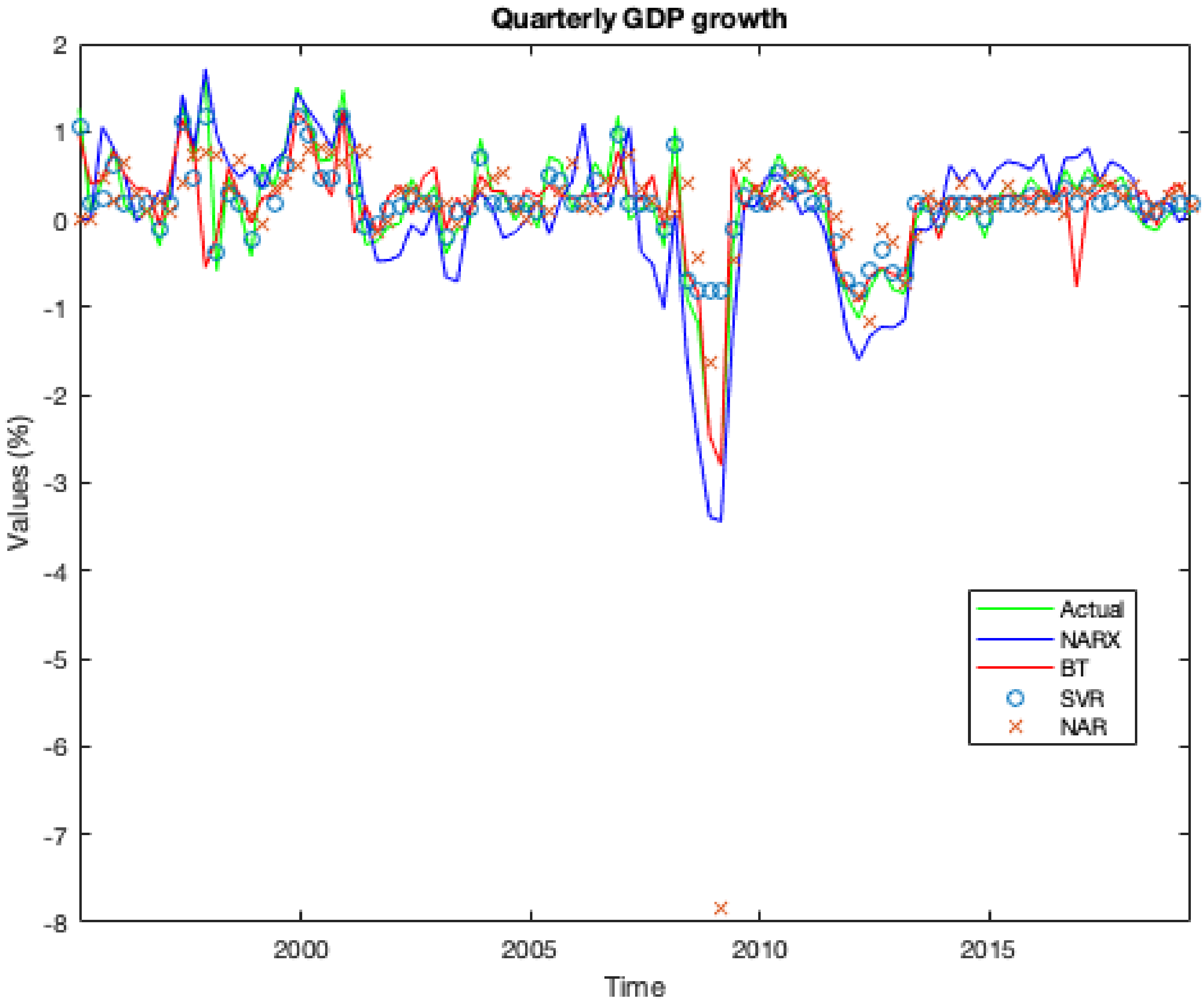
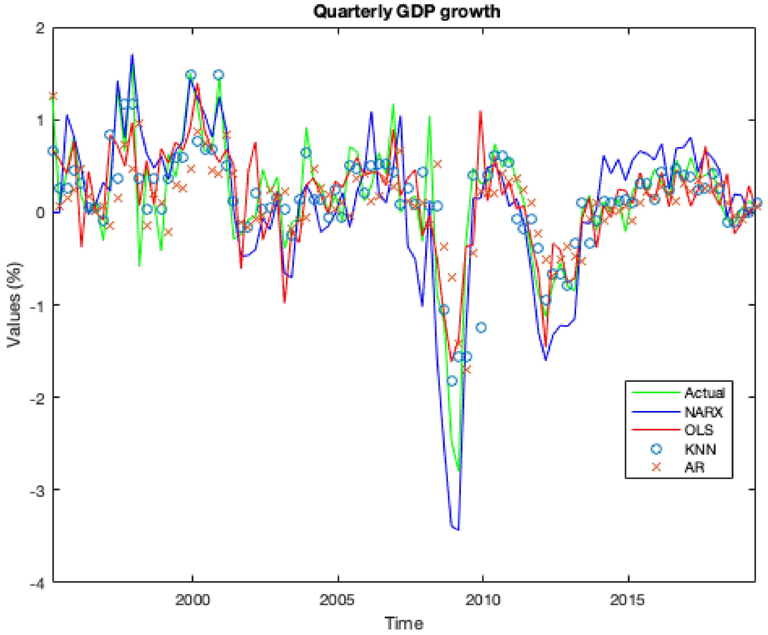
Figure 11 and in
Figure 12 it was able to correctly forecast the recession period at the beginning of the millennium and the two crises. In particular, regarding the two crises, the model forecast the upcoming recession two (for the 2008 ones) and one (for the 2011 ones) quarters before that they take place.
In the
Table 2, we report the values of the real GDP growth rate published by OECD and the relative values predicted by our models for the relative period of the two crises by combining the forecasts of all ML models with the current GDP value. The results indicate that the NARX model is able to predict GDP trends one or two quarters ahead of the start of the event. In addition, it is able to avoid false positives, that is, temporary phases of recession (only one quarter). On the other hand, the AR model is not a good predictor of the future trend of GDP both for predicting GDP variations (in intensity) and for being always behind the evolution of the economic cycle.
As we can see in the summary
Table 3, our proposed NARX model provided significant performance for our dataset when compared with other popular regression models. The two main ML models that came close to NARX performance were BT and SVR, that achieved an overall accuracy of close to 80 per cent and reduced average forecasting errors by about 0.003 per cent while KNN was unable to predict recessionary periods, although they improved accuracy by 31 per cent compared to the AR benchmark. The fourth and fifth columns show us the DM test statistics and the
p-value of the DM test statistics to test the significance of forecast accuracy for each model compared to the OLS model taken as benchmark. As we can see there is no significant difference between the ML and statistical forecasts. This means that the null hypothesis is rejected and, by considering MSE, ML models have better performances in terms of accuracy.
The performance obtained by the several models previously demonstrates how the traditional econometric tools—the linear regression model - is not sufficient to obtain remarkable performances compared to the more modern ML techniques. Indeed, NAR, SVR and NARX get better results and as previously reported, the simple auto-regression model is theoretically more robust. The results, however, must be treated with caution given our small sample size of 98 observations. So, we believe that it is necessary to consider other explanatory variables to obtain a higher level of accuracy.
6. Conclusions and Research Perspectives
The model proposed tried to replicate the actual forecasting situation for the Italian economy for the period span from the period of 1995:Q1 to 2019:Q2. We use several economic variables in order to make a prediction. The results that we obtained by our research did not make use of any data optimization by using simply the raw input parameters for all our ML models and linear regression model. Thanks to the dataset chosen as previously explained, it allowed us to obtain a good fitting. Even if persists an unexplained component that the linear regression model was not able to explain per sé, it was able to predict the two main crises in the period under research, the 2008 subprime mortgage crisis and the 2011 sovereign debt crisis. Implementing the ML techniques, we were able to increase the accuracy of our results. In particular, the non-linear regression model with exogenous variables was able to forecast not just the event but also the strength of these events. The results of the DM test confirm the superior performance of the ML models over the OLS taken as a benchmark statistical model. We are now working in comparing the ML analysis with a more classical approach using time-varying factors in the modelization. The main limit to improve this technique is the lack of officially published data. Indeed, ISTAT and other organization, such as OECD, published these data just since 1995. However, we are confident that these techniques providing better and prompt information to policy makers in making reliable predictions of recession periods and to allow them to issue all the necessary measures act to overcome the situation reducing the negative effect of the recession on all economic aspect. We believe that the bunch of ML techniques will ensure and support further research in this field. In particular, Deep Learning and Ensemble ML could support macroeconomists to have a prompt and highest quality insight into the future movement of GDP. The authors planned to investigate in this direction in the next future.


