Article

Deep Hybrid Model Based on EMD with Classification by Frequency Characteristics for Long-Term Air Quality Prediction

1
School of Computer and Information Engineering, Beijing Technology and Business University, Beijing 100048, China
2
China Light Industry Key Laboratory of Industrial Internet and Big Data, Beijing Technology and Business University, Beijing 100048, China
3
Beijing Key Laboratory of Big Data Technology for Food Safety, Beijing Technology and Business University, Beijing 100048, China
*
Authors to whom correspondence should be addressed.
Mathematics 2020, 8(2), 214; https://doi.org/10.3390/math8020214
Submission received: 10 January 2020 / Revised: 3 February 2020 / Accepted: 5 February 2020 / Published: 7 February 2020
(This article belongs to the Special Issue Advances in Machine Learning Prediction Models)

Abstract

:
Air pollution (mainly PM2.5) is one of the main environmental problems about air quality. Air pollution prediction and early warning is a prerequisite for air pollution prevention and control. However, it is not easy to accurately predict the long-term trend because the collected PM2.5 data have complex nonlinearity with multiple components of different frequency characteristics. This study proposes a hybrid deep learning predictor, in which the PM2.5 data are decomposed into components by empirical mode decomposition (EMD) firstly, and a convolutional neural network (CNN) is built to classify all the components into a fixed number of groups based on the frequency characteristics. Then, a gated-recurrent-unit (GRU) network is trained for each group as the sub-predictor, and the results from the three GRUs are fused to obtain the prediction result. Experiments based on the PM2.5 data from Beijing verify the proposed model, and the prediction results show that the decomposition and classification can develop the accuracy of the proposed predictor for air pollution prediction greatly.

1. Introduction

With the rapid development of industrialization and urbanization, urban air pollution has become increasingly serious, which has affected the living environment and health greatly. Presently, air quality monitoring stations can record hourly data to monitor the city’s PM2.5 and other air pollutants. Based on the collected data, the prediction of air pollution and the evolution of PM2.5 concentration are considered to be a key issue of air quality monitoring task for environmental air protection and governance [1].
The accurate long-term prediction can have more time to deal with air pollution in advance, so comparing the short-term prediction, the long-term prediction of air quality is more important. While the air quality data, such as PM2.5, PM10, SO2, etc., are complex nonlinear time series data with multiple components of different frequency characteristics, the long-term prediction is still an open research issue.
The prediction methods have been widely used for the time series data. In general, time series prediction methods can be roughly divided into two categories: traditional probabilistic methods [2] and machine learning models [3]. The disadvantage of the traditional time series prediction method is that the model parameters need to be determined based on theoretical assumptions and prior knowledge of the data. However, when the actual distribution of the data does not match the model’s assumptions, it will not be able to give accurate long-term prediction results.
Unlike traditional time series prediction methods, machine learning methods do not require prior physical information or linear assumptions. As long as the historical data is known, based on preset rules and algorithms, model parameters can be learned and hidden relationships and knowledge between the data can be obtained. The deep learning networks have exceeded traditional time series prediction methods in many non-linear modeling fields.
Although in theory, deep learning networks can model any complex non-linear time-series data, the deep learning network cannot obtain sufficient accuracy long-term prediction for the prediction of PM2.5 data due to the limitation of the amount of training data and the size of the network. In the following Section 2, we will describe the related works about the current prediction methods for time series data and discuss the pros and cons of traditional probabilistic methods and machine learning models. At the end of Section 2, the innovative contributions of this paper are discussed. Then, Section 3 introduces each part of the proposed predictor. Experimental results of the proposed predictor are shown and evaluated in Section 4, and finally, Section 5 presents our conclusion.

2. Related Works

Traditional methods include chemical analysis models and prediction models based on statistical theory. In the physical models, the equations are established based on the physical relationships between variables, and then the prediction models analyze and predict time series data [2]. The statistical models used include the autoregressive moving average (ARMA) [4,5,6], autoregressive integrated moving average (ARIMA) [7], threshold autoregressive (TAR) model [8], hidden Markov model (HMM) [9], etc. In [10], Berrocal et al. had discussed geostatistical techniques, such as kriging, and spatial statistical models that use the information contained in air quality model outputs, such as statistical downscaling models.
These traditional time series prediction methods determine the model parameters based on theoretical assumptions and prior knowledge of the data. However, it is often difficult to know the prior parameters because of the lack of background knowledge. When the data distribution does not match the model’s hypothesis, it will cause a mismatch between the model and the data, which seriously affects the accuracy of the prediction. Therefore, the traditional methods are less applied in the complex application of the environment.
Different from traditional time series prediction methods, machine learning methods require no prior physical information or linear assumptions. These methods build prediction models based on learning algorithms and historical data and perform operations based on preset rules and algorithms to adaptively learn model parameters and obtain hidden relationships and knowledge between data. The trained model is then used to predict the future development trends and patterns of time series data. The prediction is based on mathematical models and some parameter identification methods can be used, such as iterative algorithms [11,12,13], particle-based algorithms [14], and recursive algorithms [15,16,17].
Regression models initially were used for predictive tasks. Tang et al. [18] applied a linear regression method to predict PM2.5 emissions in the Northeast United States from 2002 to 2013 based on fine-resolution aerosol optical depth. Oteros et al. [19] used different factors of pollen concentration and took into account the extreme weather events in the Mediterranean climate characteristics to establish a multivariate regression model. Donnelly et al. [20] presented a real-time approach based on multiple linear regression for air quality prediction. While these linear regression models all faced challenges in prediction tasks with highly nonlinear time series data.
The shallow network, such as artificial neural networks (ANNs), ensemble extreme learning machine and gradient boosting machine play a key role in solving nonlinear problems [21,22,23,24]. Ni et al. [25] developed a short-term prediction method based on a back-propagation (BP) neural network for PM2.5 concentrations data such as meteorological data, including regional average rainfall, daily mean temperature, average relative humidity, average wind speed, maximum wind speed, and other pollutant concentration data, including CO, NO2, SO2, PM10, etc. In [26], a prediction model based on classification and regression tree and ensemble extreme learning machine methods were developed to split the dataset into subsets in a hierarchical fashion and build a prediction model for each leaf. Bai et al. studied the combined prediction method of shallow nonlinear autoregressive network (NAR) on the basis of BP [27], and proposed the prediction method from time and space dimensions by using shallow networks [28]. Du et al. [29] developed the geographically-weighted gradient boosting machine to address the spatial non-stationarity of the relationships between PM2.5 concentrations based on aerosol optical depth (AOD) and meteorological conditions. The above results show that these machine learning methods, which are mainly structured with shallow network features, can only obtain accurate results in short-term prediction. The reason is that its network structure is relatively simple and can only obtain short-term changes. Therefore, if we want to achieve accurate long-term prediction performance, we must use more complex networks that can capture long-term changes.
Comparing with the shallow network, the so-called deep learning networks had shown the outstanding ability for the complex time series relation. Recurrent neural network (RNN) [30] for time series prediction has attracted extensive attention from researchers because it could capture the high nonlinearity of time series data. Yadav et al. [31] predicted hourly/daily/monthly average solar radiation by an RNN, and an adaptive learning rate for the RNN was proposed. The approach was found promising when compared to the multilayer perceptron. As an improved version of the RNN, long short-term memory (LSTM), replaced it as a popular time-series data prediction technology [32,33]. The gated recurrent unit (GRU) [34] inherits the advantages of LSTM to automatically learn features and efficiently model long-term dependent information, and it also exhibits a significant increase in computational speed.
Though the deep learning model can extract more accurate information from complex environments, however, the accuracy of long-term prediction still needs to be developed further, because PM2.5 concentration series has the characteristics of randomness, strong non-linearity and non-stationarity due to the influence of meteorological factors and atmospheric pollutants. As for the air quality, the long-term precision prediction, which we mean predicting 20 to 30 steps ahead hourly, is more meaningful for the management of environmental air protection and governance. Therefore, how to obtain an accurate long-term prediction has been a considerate research field.
The researchers have found that PM2.5 data have complex nonlinearities with multiple components of different frequency characteristics [35]. In recent years, the combined methods based on data decomposition have been proven effective in improving the prediction performance, and various hybrid models have been introduced to predict nonlinear time series data.
For example, wavelet decomposition [36,37] decomposed the data into multi-dimensional information by setting suitable wavelet basis function, then, to predict each sequence and reconstruct the prediction. Another decomposition method, seasonal trend decomposition procedure based on loess (STL) [38,39] can give the seasonal components, which has been used to model air pollen for short-term predict. In our previous research, we also proposed an integrated predictor for PM2.5 long-term prediction based on STL [35], in which, we used STL to decompose PM2.5 into three components, i.e., trend, period and residual component, and ARIMA was used to model for trend component, two GRU networks for period component and residual, respectively.
Different from wavelet decomposition and STL, empirical mode decomposition (EMD) can decompose the time series data into intrinsic mode function (IMF) components with different frequency characteristics features [40]. Each component obtained by EMD is a local characteristic signal based on different time scales of the original time series itself, representing each frequency component in the original signal, and arranged in order from high frequency to low frequency, which are independent of each other. The process of EMD decomposition is actually the simplification of complex time series. In [41], the decomposition process of EMD was regarded as a denoising procedure of training data, and the prediction results were obtained by support vector regression (SVR) based on different feature vectors. The results showed the superiority of the model in power load prediction. In some other studies, prediction methods combined with EMD treated the first high-frequency IMF sequence, which did not contribute to the prediction result, as a noise term and discarded it [42,43].
Qiu et al. [44] presented an integrated method based on an EMD algorithm and a deep learning method, in which the load demand sequence was first decomposed into several IMFs. Then, the extracted IMFs were modeled using a deep belief network (DBN) containing two restricted Boltzmann machines (RBMs) to accurately predict the evolution of each IMF. The predictions of each model were finally combined by an additional operation to obtain the total output of the load demand. Wang et al. [45] introduced a feedforward neural network (FNN) into the prediction framework based on EMD, proposed a weighted reorganization strategy, and conducted a single-step prediction experiment on four nonlinear nonstationary sequences to verify and compare the effectiveness of the proposed model. Bedi et al. [46] combined EMD with LSTM to estimate the electricity demand for a given time interval. The performance of the proposed approach was evaluated by comparison with the prediction results of RNN and EMD with RNN models.
The above-combined models [44,45,46] were based on such a framework, that is, the original time series data was first decomposed into several IMFs and one residue by the EMD method. Then, the predicted model, such as LSTM, was applied to each IMF including the residue independently. Finally, the prediction results of all IMFs were aggregated by simply summed to produce an ensemble prediction of the original time series. We must mention that because the frequency components in each segment are different, the number of IMF components obtained by EMD decomposition is also different. This can result in different numbers of trained and online predicted models, but the above references do not explain how to solve this problem.
Significantly different from previous studies, we will combine IMF components to achieve the unification of the training model and prediction model in practical applications. Our innovative contributions are highlighted as follows.
(1)
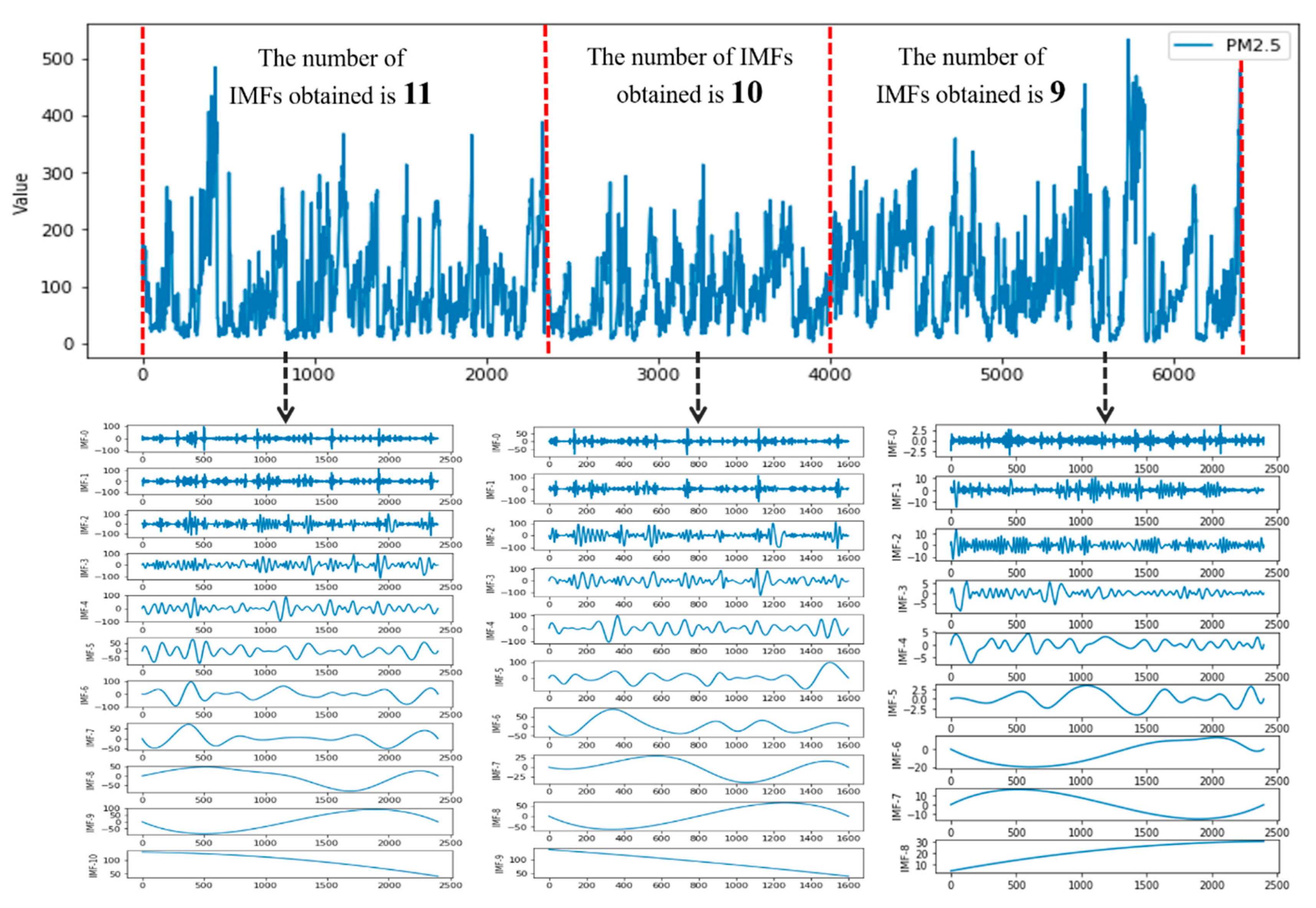
After EMD, the obtained IMF components are further analyzed for their frequency characteristics, and all the components are divided into a fixed number of groups by convolutional neural network (CNN) networks. Different from [44,45,46], the fixed number can effectively solve the problem that a variable number of IMF components will be obtained when predicting different time intervals.
(2)
We present a general framework that predicts the PM2.5 data from air quality monitoring systems and obtains accurate long-term predictions that can meet the needs of precision in air quality warning.

3. Hybrid Deep Predictor

The proposed predictor has a hybrid structure, in which the data are decomposed by EMD to reduce their nonlinear complexity, and then the IMFs’ frequency characteristics are analyzed, and all the components are divided into a fixed number of groups by CNN networks. For each group, the deep learning network GRU is used to model and predict, and finally, all the predictions of GRU are added to obtain the prediction result. Next, we will detail each part of the proposed model and provide its flowchart.

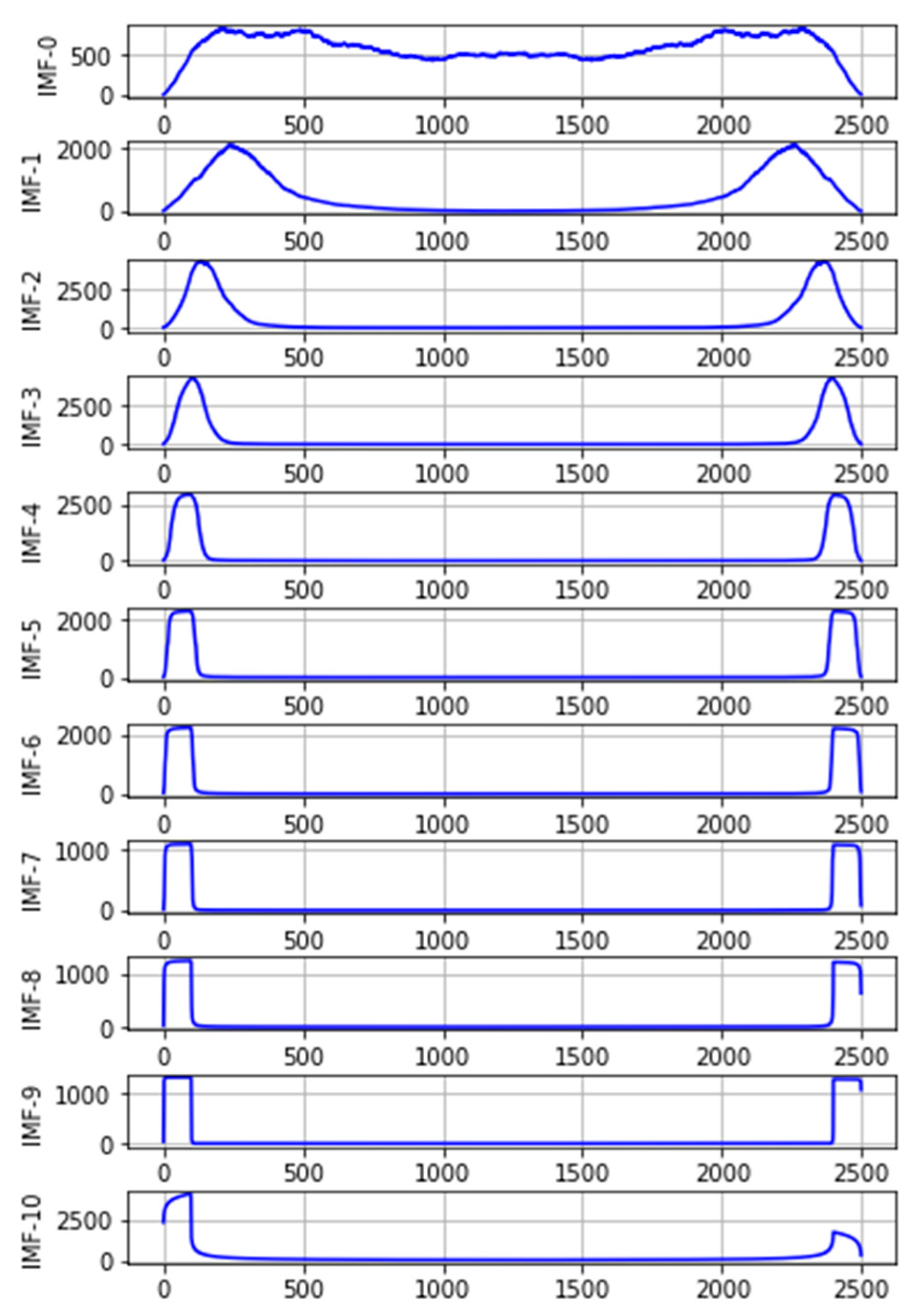
3.1. Decomposition and Analysis of PM2.5 Time Series

EMD decomposes complex signals into a finite number of IMFs automatically based on the frequency characteristics of the data, and the decomposed IMF components contain local characteristic information of different timescales of the original signal, which should satisfy the following conditions: (1) over the entire time range, the absolute value of the difference between the number of zero crossings and the number of extreme points is equal to 0 or 1; and (2) the mean value of the envelope constructed by local maxima and minima must be zero at any point. EMD is an adaptive data processing or mining method and is essentially a smoothing process for time series data (or signals). It can theoretically be applied to the decomposition of any type of time series (or signal).
Assume D t is the time series to be decomposed, h e is the expected decomposition result to be obtained. The decomposition process is as follows [47]:
(1)
Identify the local maximum point of the given time series data D t and fit the maximum point with a cubic spline interpolation function to form an upper envelope of the original data.
(2)
Similarly, find the local minimum point of D t and fit all the minimum points through the cubic spline interpolation function to form the lower envelope of the original data.
(3)
Calculate the mean of the upper envelope and the lower envelope, denoted as m e .
(4)
Subtract the average m e of the envelope from the original data sequence D t to obtain a new data sequence h e : h e = D t m e .
(5)
Repeat steps 1-4 with h e until one of the following stop criteria is met: ①, the preset maximum number of iterations is reached; ②, the last IMF separated is small; ③, the maximum or minimum value of the signal is less than 2; ④, h e is monotonic curve.
(6)
Treat h e as an IMF, and calculate the remainder R t = D t h e .
(7)
Use R t as the new D t , and repeat steps (1)–(6) until all IMFs are obtained.
In the above decomposition algorithm, is the average value of the upper envelope and the lower envelope, represents the difference between the sequence and the IMF. The traditional EMD algorithm performs spline interpolation on the extreme points, making the derivative at the boundary of the IMF component large, and resulting in an end defect. Therefore, in this study, the first point and endpoint of the sequence curve were added as extreme points to the spline to avoid the end defect.
To show the time and frequency domain characteristics of different components, we take PM2.5 data with 2500 samples from the air quality monitoring systems as an example to give the results of EMD decomposition. In Figure 1a, all the obtained IMFs are shown in the time domain (from IMF-0 to IMF-10), and correspondingly, each sub-picture on the right-hand side, Figure 1b is the transformed component of the frequency domain by the fast Fourier transform (FFT). It can be seen from Figure 2 that each IMF has a specific time domain and frequency domain correspondence, and the frequency components contained in the IMF are reduced from top to bottom.
To further illustrate the different frequency components contained in each IMF, we perform a one-dimensional convolution operation on each IMF in the frequency domain. The convolution formula is as follow:
f ( x ) * g ( x ) = + f ( τ ) * g ( x τ ) d τ ,
where f ( x ) is the convolved function, and g ( x ) is the convolution kernel function. The result of the one-dimensional convolution is equal to the integral of the integrand function f ( τ ) * g ( x τ ) on the interval ( , + ) and the convolution kernel g ( x ) is selected as a Gaussian kernel function.
The results of the convolution of IMFs and the Gaussian kernel function g ( x ) are shown in Figure 2. It can be clearly seen that the IMF-0 component contains a wider band of frequency components. In contrast, the frequency components contained in IMF-1 and IMF-2 are significantly reduced, but there are still long tails in the cutoff band. Differently, as for IMF-3 and IMF-4, the downhill is significantly steeper, indicating that fewer frequency components are included. Furthermore, for IMF-5–10, the downslope is almost vertical, and we can find that the fluctuations of these components in the time domain map (Figure 1a) are relatively flat.
It can be seen that the frequency characteristics of the IMFs are different. Compared to the original data, each IMF only contains partial frequency components. Therefore, after decomposing and predicting each component separately, more accurate prediction results can be obtained.
Moreover, we found that the number of IMFs varies for different time periods. The decomposition result of the EMD algorithm depends on the original time series itself. The number of IMFs obtained by EMD is usually different within different prediction intervals. As shown in Figure 3, we performed EMD on the three different data intervals [0, 2400), [2400, 4000), and [4000, 6400) of thePM2.5 data, and the number of IMFs obtained was 11, 10, and 9, respectively.
We can note that the number of trained prediction sub-models will be different from the number of IMF components in the different prediction intervals. Therefore, it is necessary to combine an unfixed number of IMFs into a fixed number according to frequency characteristics.
In this study, according to the respective frequency characteristics of IMFs, we combined all the IMFs into a fixed number of groups. That is to say, the decomposition components having similar frequency characteristics will be labeled, grouped and added together, then for each group, one model will be trained. Therefore, the number of models in each prediction interval will be fixed.

3.2. Classification and Combination for IMFs

Convolution calculation can effectively capture the dynamic change of the signal and obtain the mode characteristics of its change. This method has achieved good results in many pattern recognition applications, so we would use the CNN neural network to classify and group IMFs.
The IMF components to be processed in this study are one-dimensional discrete time series. Therefore, we use one-dimensional convolution as the convolutional layer to construct one-dimensional CNN, which is suitable for feature extraction from IMF sequences. Given an input IMF sequence X t , t = 1 , , n , and the convolution kernel function, the filters sequentially perform a local convolution operation on the input features of the previous layer. The output of the convolution is as follows:
x t = l = 1 m k l × X t l + 1 .
The convolutional layer needs an activation function f ( ) for nonlinear feature mapping. In this study, the rectified linear unit (ReLU) with fast convergence speed is selected as the activation function. The formula is as follows:
f ( x t ) = { 0 , x t 0 x t , x t > 0
Then by flattening and full connection process [48], a one-dimensional convolutional neural network extracts the frequency characteristics of the IMFs, the Softmax classifier, classifies the features and finally achieves the network output, i.e., the labels of each IMF. The schematic of the one-dimensional CNN is shown in Figure 4, where X t is the input IMF sequence, and y is the output label of each IMF. In consequence, the IMFs in each group will be added (noted as S t ) and as the input data for the GRU network.

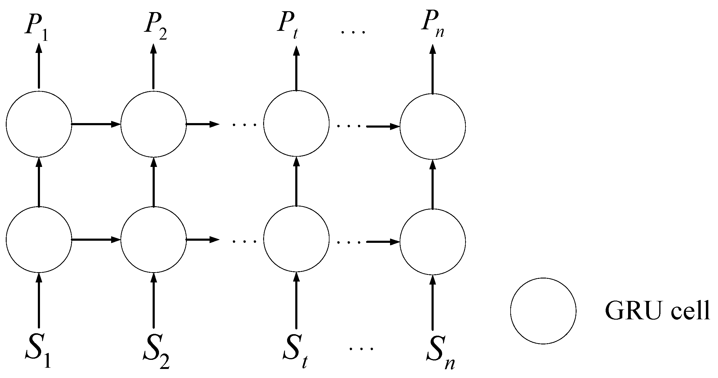
3.3. Deep Prediction Network for Combined IMFs

In this study, the GRU network was designed to train and predict the IMFs groups. Using the known input and output data, the network is trained by the stochastic gradient descent algorithm, and the optimal weight can be obtained. The GRU network was trained on the sum of IMFs sequences in each group. The GRU network consisted of multiple GRU cells, and here the number of hidden layers is set as 2. Shown as Figure 5, S t , t = 1 , 2 , , n is the input of the GRU network, P t   , t = 1 , 2 , , n is the output.
GRU uses the update gate to control the degree to which the state information of the previous moment is brought into the current state. The larger the value of the update gate, the more the state information is brought in from the previous moment. The reset gate is similar to the forget gate in LSTM, which is used to control the degree of ignoring the state information of the previous moment. The smaller the reset gate value, the more the information neglected.
The forward propagation formulas in each GRU cell are as follows [49]:
z t = σ ( a t U z + h t 1 W z + b z ) r t = σ ( a t U r + h t 1 W r + b r ) h ˜ t = tanh ( a t U h + ( h t 1 r t ) W h + b h ) h t = ( 1 z t ) h ˜ t + z t h t 1
where a t R d is the input vector to each GRU cell; z t , r t , h ˜ t , and h t stand for the update gate, reset gate, candidate state of the current hidden node, and the active state of the current hidden node output at time t , respectively; U and W are weight matrices to be learned during model training; b represents bias vectors; is an element-wise multiplication; and σ and tanh are activation functions. The GRU is trained by the gradient descent algorithm, and the parameters are continually updated until convergence. The proposed methods proposed in this paper can combine other identification approaches [50] to study the modeling and prediction problems applied to other fields [51,52] such as internet of things systems [53,54] and water environment prediction and management control [55,56].

3.4. Hybrid Model Framework
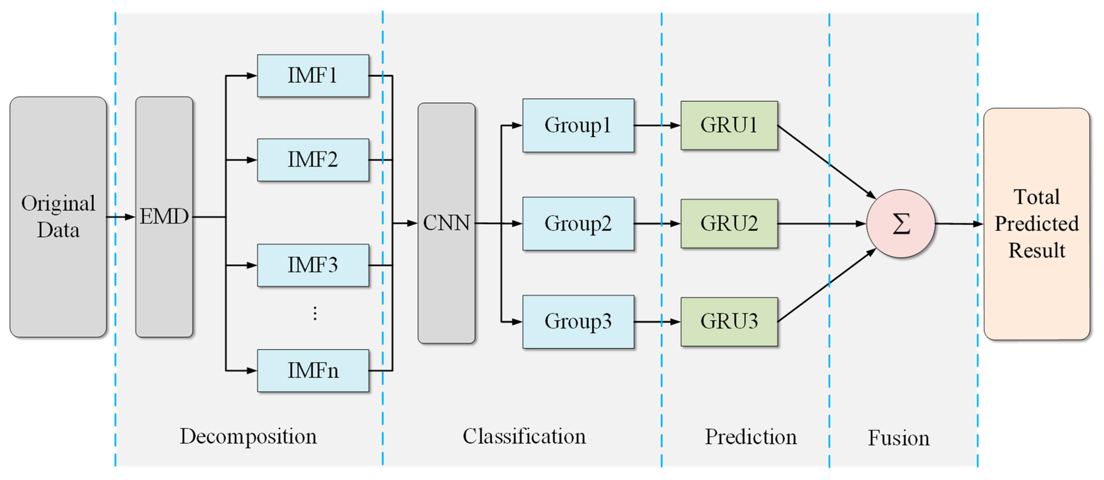
In conclusion, based on the discussion in Section 3.1, Section 3.2 and Section 3.3, the proposed deep learning predictor is shown in Figure 6. The number of groups is fixed at three, which is a result of the experiment. We have used the PM2.5 data from an air quality monitoring system to verify the proposed predictor, and this shows that the three groups of IMFs can maintain high performance at a low calculation cost.
The hybrid predictor includes the two processes of training and predicting. The first process is to train the CNN and GRU based on the IMFs decomposed by EMD. The details are as follows:
(1)
Decompose the data into IMFs by EMD and label each IMF into three groups based on its frequency characteristics as Group1–3.
(2)
Train the CNN by IMFs and labels, and add the sequences to each group.
(3)
Train GRU models for each group to get three GRU sub-predictors.
The predicting process is to predict the future trends of data by the trained networks, and it is implemented as follows:
(1)
Decompose the input data into IMFs by EMD.
(2)
Use CNN to classify IMFs into three groups, and add the sequences of the same group together.
(3)
Use GRU models to obtain the predictions of all the groups.
(4)
Fuse all the predictions to obtain the integrated output of the original time series.

4. Experiment Results and Discussion

4.1. Dataset and Experimental Setup

Our experiments are based on the PM2.5 dataset, which is from the US Department of State [57]. The dataset includes 37,704 records of hourly PM2.5 average concentration data in Beijing from January 2013 to December 2017. To assess the prediction performance of the different models, we selected the first 75% of the data for training and the remaining 25% for testing. The rang of the test data is from 2 μ g / m 3 to 601 μ g / m 3 .
The open-source deep learning library Keras, based on TensorFlow, was used to build all of the learning models. All of the experiments were performed on a PC server with an Intel CORE CPU i5-4200U at 1.60 GHz, with 4 GB of memory. The default parameters in Keras were used for deep neural network initialization (e.g., weight initialization). The ReLU was used as the activation function of the CNN, which was set with 32 convolution kernels in each layer. The group labels were set by one-hot encoding. For the sub-predictors, we designed GRU networks with two hidden layers, and the Adam algorithm was selected as GRU’s optimized method.
In the experiments, the long-term prediction with 24 steps ahead was considered, in which we used the PM2.5 data during the previous 24 h to predict the next 24 h. In order to compare the accuracy performance of the proposed predictor, five evaluation indicators are used, such as root mean square error (RMSE), normalized root mean square error (NRMSE), mean absolute error (MAE), symmetric mean absolute percentage error (SMAPE), Pearson correlation coefficient (R) whose calculation formula are shown in Equations (5)–(9).
R M S E = i = 1 N ( x p r e ( i ) x o b s ( i ) ) 2 N
N R M S E = 1 max ( x p r e ) min ( x p r e ) i = 1 N ( x p r e ( i ) x o b s ( i ) ) 2 N
M A E = 1 N i = 1 N | x p r e ( i ) x o b s ( i ) |
S M A P E = 1 N i = 1 N | x o b s ( i ) x p r e ( i ) | ( | x o b s ( i ) | + | x p r e ( i ) | ) / 2
R = i = 1 N ( x o b s ( i ) x ¯ o b s ( i ) ) ( x p r e ( i ) x ¯ p r e ( i ) ) i = 1 N ( x o b s ( i ) x ¯ o b s ( i ) ) 2 i = 1 N ( x p r e ( i ) x ¯ p r e ( i ) ) 2 ,
where N is the number of predictive datasets; x o b s represents PM2.5 data, namely, the ground truth value and x p r e is the predicted value; max ( x p r e ) represents the maximum of predictive data; min ( x p r e ) represents the minimum of predictive data; x ¯ o b s represents the average of PM2.5 and x ¯ p r e represents the average of prediction.
The comparison of the two cases shows that our proposed model is effective in predicting PM2.5. From Case 1 (Section 4.2), it can be seen that the decomposition and prediction using EMD technology is effective. In Case 2 (in Section 4.3), by comparing with the results of different combinations of IMF components, the results show that the proposed combination method has advantages in PM2.5′s long-term prediction.

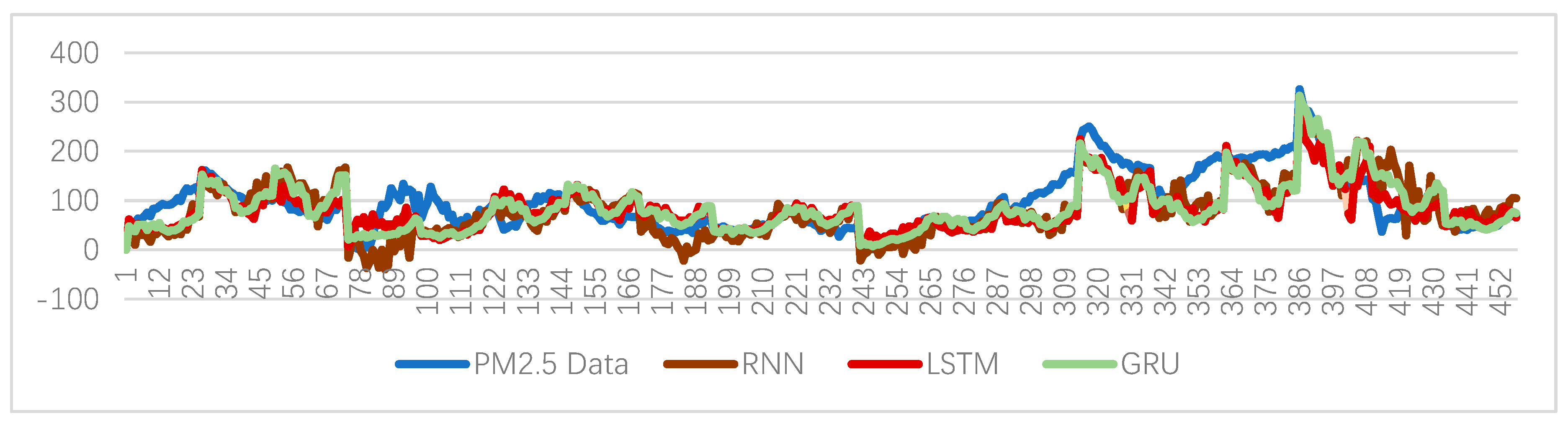
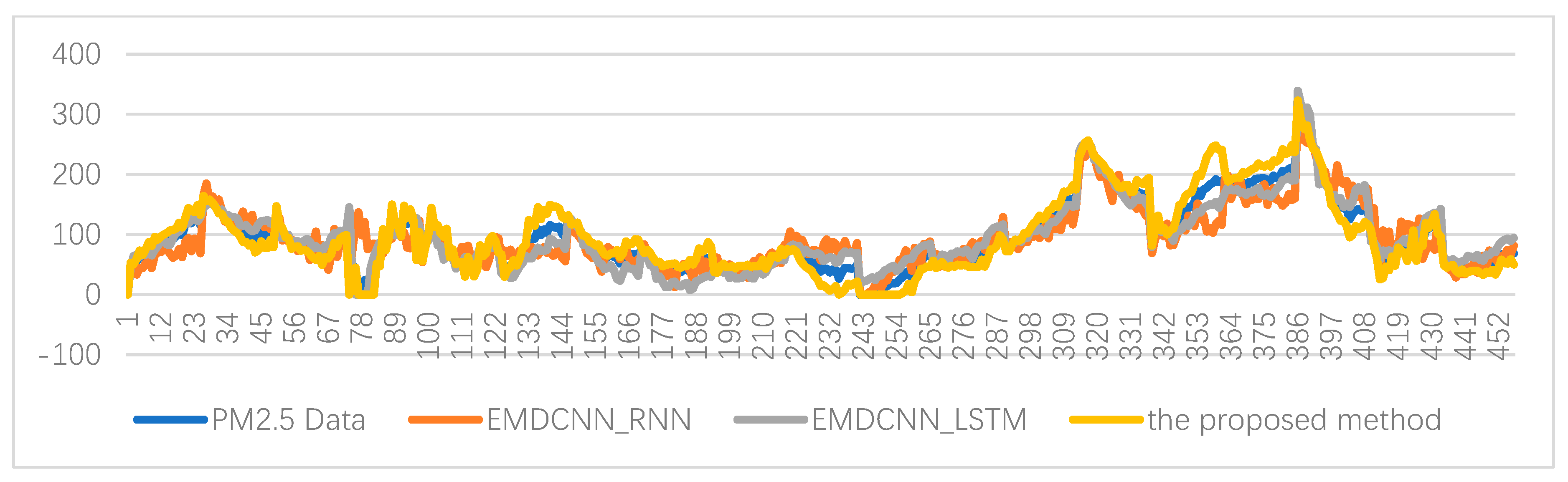
4.2. Case 1: Prediction Performance Analysis of Different Predictor

In this experiment, in addition to the proposed method, six other models are used to predict 24 h ahead of the PM2.5 average concentration, which are RNN [31], LSTM [32], GRU [34], Decomposition-ARIMA-GRU-GRU [35], and after decomposing the data by EMD and classification of CNN firstly, RNN [31] and LSTM [32] as the sub-predictors, respectively. The PM2.5 data introduced in Section 4.1 is used to show the prediction result. Figure 7 and Figure 8 give the predictions of hourly PM2.5 average concentration data in Beijing from 1 to 20 December, 2017 by RNN [31], LSTM [32], GRU [33], EMDCNN_RNN (EMD and CNN-based RNN), EMDCNN_LSTM (EMD and CNN-based LSTM), and the proposed method.
To evaluate the performance of each method numerically, Table 1 gives a comparison of the prediction results in terms of RMSE, NRMSE, MAE, SMAPE, and R. The smaller the values of RMSE, NRMSE, MAE, SMAPE, the more accurate the predictions. A higher value of R indicates a better fit between prediction and observation. It is apparent from the comparison of prediction results that the decomposition models are significantly outperformed than the undecomposed ones, and the proposed EMDCNN_GRU model has a more accurate prediction than other models with the smallest RMSE, NRMSE, MAE, SMAPE. The correlation coefficient, R, of the EMDCNN_GRU model is above 0.8.
Compared with our previous work Decomposition-ARIMA-GRU-GRU model [35], the prediction RMSE, NRMSE, MAE, SMAPE of the proposed EMDCNN_GRU model for PM2.5 are approximately 9.61%, 12.27%, 14.61%, 4.94% lower, respectively, and the R coefficient is approximately increased by 5.63%.
The results show that it can effectively improve the accuracy of prediction results to decompose PM2.5 into multiple components as the RMSEs can be significantly reduced. The reason is that affected by weather, pollution emissions, and regional relationships, PM2.5 contains multiple components, which makes long-term prediction difficult. The modeling of the decomposed components can reduce the difficulty, so that the prediction accuracy of each component can be guaranteed, and the accuracy of the prediction results can be improved. Moreover, for each component, more accurate modeling is necessary. The more accurate prediction result obtained by each component, the more accurate the final prediction result will be. Therefore, we found that different sub-predictor can obtain different prediction results. Consistent with many research results, GRU is better than LSTM and RNN.

4.3. Case 2: Prediction Performance Analysis of Different Combinations for IMFs

In this experiment, the collected hourly PM2.5 data in Beijing from January, 2013 to December, 2017 are used to show the prediction result. We will conclude that mode No. 5 including three groups with Group1: {IMF 0–2}, Group2: {IMF 3–4}, Group3: {IMF 5–10} is the suitable mode in long-term prediction (24-h ahead) for PM2.5.
Table 2 lists the prediction performances of 12 different modes. For each mode, we used adifferent combination mode to train the CNN, and obtained a different number of groups, then GRUs are trained for each group. The details are as follows, and a parenthesis represents a group, several parentheses indicate that several GRU sub-predictors need to be built.
(1)
Mode No. 1: IMFs is divided into a group, i.e., {IMF 1–10}. Removing noise term, IMF0, others use one GRU to predict;
(2)
Mode No. 2: do not decompose the PM2.5 data, using one GRU for prediction;
(3)
Mode No. 3: IMFs is divided into two groups, i.e., {IMF 0}, {IMF 1–10}. Using two GRUs for two sub-sequences prediction separately;
(4)
Mode No. 4: IMFs is divided into two groups, i.e., {IMF 0–2}, {IMF 3–10}. Using two GRUs for two sub-sequences prediction separately;
(5)
Mode No. 5: IMFs is divided into three groups, i.e., {IMF 0–2}, {IMF 3–4}, {IMF 5–10}. Using three GRUs for three sub-sequences prediction separately;
(6)
Mode No. 6: IMFs is divided into four groups, i.e., {IMF 0–2}, {IMF 3–4}, {IMF 5–6}, {IMF 7–10}. Using four GRUs for four sub-sequences prediction separately;
(7)
Mode No. 7: IMFs is divided into five groups, i.e., {IMF 0}, {IMF 1–2} {IMF 3–4}, {IMF 5–6}, {IMF 7–10}. Using five GRUs for five sub-sequences prediction separately;
(8)
Mode No. 8: IMFs is divided into six groups, i.e., {IMF 0}, {IMF 1–2}, {IMF 3–4}, {IMF 5–6}, {IMF 7–8}, {IMF 9–10}. Using six GRUs for six sub-sequences prediction separately;
(9)
Mode No. 9: IMFs is divided into seven groups, i.e., {IMF 0}, {IMF 1–2}, {IMF 3}, {IMF 4}, {IMF 5–6}, {IMF 7–8}, {IMF 9–10}. Using seven GRUs for seven sub-sequences prediction separately.
(10)
Mode No. 10: IMFs is divided into eight groups, i.e., {IMF 0}, {IMF 1–2}, {IMF 3}, {IMF 4}, {IMF 5}, {IMF 6}, {IMF 7–8}, {IMF 9–10}. Using eight GRUs for eight sub-sequences prediction separately;
(11)
Mode No. 11: IMFs is divided into nine groups, i.e., {IMF 0}, {IMF 1–2}, {IMF 3}, {IMF 4}, {IMF 5}, {IMF 6}, {IMF 7}, {IMF 8}, {IMF 9–10}. Using nine GRUs for nine sub-sequences prediction separately;
(12)
Mode No. 12: IMFs is divided into ten groups, i.e., {IMF 0}, {IMF 1–2}, {IMF 3}, {IMF 4}, {IMF 5}, {IMF 6}, {IMF 7}, {IMF 8}, {IMF 9}, {IMF 10}. Using ten GRUs for ten sub-sequences prediction separately.
From Table 2, we can note a large difference in performance across the different groups. The RMSE of {IMF 1–10} in mode No. 1 is 6.9% lower than mode No. 2, which indicates that removing the first IMF component (noise item) decomposed by EMD is helpful for prediction. The value of five evaluation indicators from mode No. 1 to mode No. 12 is highly variable, but the prediction error in mode No. 5, 6, and 7 is the smallest.
Mode No. 5, 6, and 7 have similar prediction performance, with RMSE reaching 46.2619, 46.0065, and 45.0356, respectively. Compared with mode No. 5, the RMSE, NRMSE, MAE, the SMAPE of mode No. 6 or 7 is slightly reduced, but we have to train 4 or 5 GRUs, so the training parameters are increased by 1/3, 2/3 respectively. The results show that the decomposition of the data is effective, while the data do not be excessively decomposed. We believe that the reason is that for each decomposition component, the prediction will produce a certain error. If too many decomposed components are used for prediction, each component will bring errors that will lead to a reduction in the accuracy of the final prediction result. In addition to the accuracy of the predictions, we believe that the amount of computation in the air quality monitoring system is also important. In order to reduce the cost of the actual system, we choose a method of calculating less. Therefore, to ensure the prediction performance and keep the cost of parameters, mode No. 5 with three groups is a suitable choice for the PM2.5 data of the application in the air quality monitoring system.
Further, from the comparison of mode 1 and mode 3, it can be seen that for PM2.5 data, the RMSE of mode 1 is 58.7715, which is smaller than 59.6399 of mode 3. However, we think this is not much different. Because the average value of PM2.5 is about 100, such a small RMSE difference cannot have a very large impact on the prediction result. Therefore, we believe that it has little reduction in the predicted final performance by using IMF0 as a component for prediction or discarding it as just noise. We think that the reasons may be that the PM2.5 data is so-called chaotic data, therefore, the removal of noise cannot fundamentally improve prediction performance. Therefore, in the proposed prediction structure, IMF0 is not regarded as noise and discarded.

5. Conclusions

In recent years, environmental problems such as PM2.5 have seriously affected people’s normal lives, and air quality has begun to receive more and more public attention. Due to the influence of meteorological factors and atmospheric pollutants, the PM2.5 concentration series has the characteristics of randomness, strong non-linearity, and non-stationarity with multiple components of different frequency characteristics. Therefore, accurate long-term prediction is still a challenge.
This study proposes a hybrid deep learning predictor based on EMD and GRU group model to predict complex PM2.5 concentration time series. The key issue is to combine the IMF components obtained by the EMD algorithm, so as to solve the problem of inconsistent IMF components in different periods of time series and improve the precision of prediction. A CNN was used to classify IMFs into groups based on the frequency feature, and the GRUs were trained as the sub-predictors for separate predictions. The prediction results of the sub-predictor are finally added to obtain the final prediction result. The proposed predictor can obtain accurate predictions for the next 24 h, which can provide the advantage information for air pollution prevention and management in advance.
The proposed method has universal characteristics and can be used for the prediction of other data, such as meteorological data, such as air temperature, wind speed, relative humidity and other air pollutant measurements, such as PM10, SO2, etc.

Author Contributions

Conceptualization, X.-B.J. and N.-X.Y.; data curation, Y.-T.B. and T.-L.S.; formal analysis, J.-L.K.; methodology, X.-B.J. and N.-X.Y.; software, N.-X.Y.; Supervision, X.-Y.W., Y.-T.B., T.-L.S. and J.-L.K.; validation, X.-Y.W., Y.-T.B. and T.-L.S.; validation, N.-X.Y.; writing—original draft, X.-B.J. and N.-X.Y.; writing—review and editing, X.-B.J. and N.-X.Y. All authors have read and agree to the published version of the manuscript.

Funding

This work was supported in part by the National Key Research and Development Program of China no. 2017YFC1600605, National Natural Science Foundation of China, No. 61673002, 61903009, 61903008, Beijing Municipal Education Commission, No. KM201910011010, KM201810011005, Young Teacher Research Foundation Project of BTBU No. QNJJ2020-26 and Beijing excellent talent training support project for young top-notch team No. 2018000026833TD01.

Conflicts of Interest

The authors declare no conflict of interest.

References

  1. Xu, J.; Yang, W.; Han, B.; Wang, M.; Wang, Z.; Zhao, Z.; Bai, Z.; Vedal, S. An advanced spatio-temporal model for particulate matter and gaseous pollutants in Beijing, China. Atmos. Environ. 2019, 211, 120–127. [Google Scholar] [CrossRef]
  2. Di, Q.; Koutrakis, P.; Schwartz, J. A hybrid prediction model for PM2.5 mass and components using a chemical transport model and land use regression. Atmos. Environ. 2016, 131, 390–399. [Google Scholar] [CrossRef]
  3. Bai, Y.; Wang, W.; Jin, X.; Su, T.; Kong, J.; Zhang, B. Adaptive filtering for MEMS gyroscope with dynamic noise model. ISA Trans. 2020. [Google Scholar] [CrossRef] [PubMed]
  4. Benmouiza, K.; Cheknane, A. Small-scale solar radiation forecasting using ARMA and nonlinear autoregressive neural network models. Theor. Appl. Climatol. 2016, 124, 945–958. [Google Scholar] [CrossRef]
  5. Kocak, C. ARMA (p,q) type high order fuzzy time series forecast method based on fuzzy logic relations. Appl. Soft Comput. 2017, 58, 92–103. [Google Scholar] [CrossRef]
  6. Perez, E.G.; Ceballos, R.F. Malaria Incidence in the Philippines: Prediction using the Autoregressive Moving Average Models. Int. J. Eng. Future Tech. 2019, 16, 1–10. [Google Scholar] [CrossRef] [Green Version]
  7. Ruby-Figueroa, R.; Saavedra, J.; Bahamonde, N.; Cassano, A. Permeate flux prediction in the ultrafiltration of fruit juices by ARIMA models. J. Membr. Sci. 2017, 524, 108–116. [Google Scholar] [CrossRef]
  8. Aero, O.; Ogundipe, A. Fiscal Deficit and Economic Growth in Nigeria: Ascertaining a Feasible Threshold. Soc. Sci. Electr. Public 2018. Available online: https://ssrn.com/abstract=2861505 (accessed on 31 December 2016).
  9. Guo, H.; Pedrycz, W.; Liu, X. Hidden Markov Models-Based Approaches to Long-term Prediction for Granular Time Series. IEEE Trans. Fuzzy Syst. 2018, 26, 2807–2817. [Google Scholar] [CrossRef]
  10. Berrocal, V.J.; Guan, Y.; Muyskens, A.; Wang, H.; Reich, B.J.; Mulholland, J.A.; Chang, H.H. A comparison of statistical and machine learning methods for creating national daily maps of ambient PM2.5 concentration. Atmos. Environ. 2019, 222, 117130. [Google Scholar] [CrossRef] [Green Version]
  11. Ding, F.; Pan, J.; Alsaedi, A.; Hayat, T. Gradient-based iterative parameter estimation algorithms for dynamical systems from observation data. Mathematics 2019, 7, 428. [Google Scholar] [CrossRef] [Green Version]
  12. Ding, F.; Lv, L.; Pan, J.; Wan, X.; Jin, X.B. Two-stage gradient-based iterative estimation methods for controlled autoregressive systems using the measurement data. Int. J. Control Autom. Syst. 2020, 18. [Google Scholar] [CrossRef]
  13. Xu, L.; Ding, F. Iterative parameter estimation for signal models based on measured data. Circuits Syst. Signal Process. 2018, 37, 3046–3069. [Google Scholar] [CrossRef]
  14. Ding, J.; Chen, J.; Lin, J.X.; Wan, L.J. Particle filtering based parameter estimation for systems with output-error type model structures. J. Frankl. Inst. 2019, 356, 5521–5540. [Google Scholar] [CrossRef]
  15. Ding, F.; Xu, L.; Meng, D.; Jin, X.B.; Alsaedi, A.; Hayat, T. Gradient estimation algorithms for the parameter identification of bilinear systems using the auxiliary model. J. Comput. Appl. Math. 2020, 369, 112575. [Google Scholar] [CrossRef]
  16. Cui, T.; Ding, F.; Jin, X.B.; Alsaedi, A.; Hayat, T. Joint multi-innovation recursive extended least squares parameter and state estimation for a class of state-space systems. Int. J. Control Autom. Syst. 2020, 18. [Google Scholar] [CrossRef]
  17. Xu, L.; Xiong, W.L.; Alsaedi, A.; Hayat, T. Hierarchical parameter estimation for the frequency response based on the dynamical window data. Int. J. Control Autom. Syst. 2018, 16, 1756–1764. [Google Scholar] [CrossRef]
  18. Tang, C.H.; Coull, B.A.; Schwartz, J.; Di, Q.; Koutrakis, P. Trends and spatial patterns of fine-resolution aerosol optical depth–derived PM2.5 emissions in the Northeast United States from 2002 to 2013. J. Air Waste Manag. Assoc. 2017, 67, 64–74. [Google Scholar] [CrossRef] [Green Version]
  19. Oteros, J.; García-Mozo, H.; Hervás, C.; Galán, C. Bioweather and autoregressive indices for predicting olive pollen intensity. Int. J. Biometeorol. 2013, 57, 307–316. [Google Scholar] [CrossRef]
  20. Donnelly, A.; Misstear, B.; Broderick, B. Real time air quality forecasting using integrated parametric and non-parametric regression techniques. Atmos. Environ. 2015, 103, 53–65. [Google Scholar] [CrossRef]
  21. Bai, Y.T.; Wang, X.Y.; Jin, X.B.; Zhao, Z.Y.; Zhang, B.H. A neuron-based kalman filter with nonlinear autoregressive model. Sensor 2020, 20, 299. [Google Scholar] [CrossRef] [Green Version]
  22. Wang, L.; Zhang, T.; Wang, X.; Jin, X.; Xu, J.; Yu, J.; Zhang, H.; Zhao, Z. An approach of improved Multivariate Timing-Random Deep Belief Net modelling for algal bloom prediction. Biosyst. Eng. 2019, 177, 130–138. [Google Scholar] [CrossRef]
  23. Zhan, Y.; Luo, Y.; Deng, X.; Chen, H.; Grieneisen, M.L.; Shen, X.; Zhu, L.; Zhang, M. Spatiotemporal prediction of continuous daily PM2.5 concentrations across China using a spatially explicit machine learning algorithm. Atmos. Environ. 2017, 155, 129–139. [Google Scholar] [CrossRef]
  24. Wang, L.; Zhang, T.; Jin, X.; Xu, J.; Wang, X.; Zhang, H.; Yu, J.; Sun, Q.; Zhao, Z.; Xie, Y. An approach of recursive timing deep belief network for algal bloom forecasting. Neural Comput. Appl. 2020, 32, 163–171. [Google Scholar] [CrossRef]
  25. Ni, X.Y.; Huang, H.; Du, W.P. Relevance analysis and short-term prediction of PM 2.5 concentrations in Beijing based on multi-source data. Atmos. Environ. 2017, 150, 146–161. [Google Scholar] [CrossRef]
  26. Shang, Z.; Deng, T.; He, J.; Duan, X. A novel model for hourly PM2.5 concentration prediction based on CART and EELM. Sci. Total Environ. 2019, 651, 3043–3052. [Google Scholar] [CrossRef]
  27. Bai, Y.; Jin, X.; Wang, X. Compound Autoregressive Network for Prediction of Multivariate Time Series. Complexity 2019, 2019, 9107167. [Google Scholar] [CrossRef]
  28. Bai, Y.; Wang, X.; Sun, Q. Spatio-Temporal Prediction for the Monitoring-Blind Area of Industrial Atmosphere Based on the Fusion Network. Int. J. Environ. Res. Public Health 2019, 16, 3788. [Google Scholar] [CrossRef] [Green Version]
  29. Du, P.; Wang, J.; Hao, Y.; Niu, T.; Yang, W. A novel hybrid model based on multi-objective Harris hawks optimization algorithm for daily PM 2.5 and PM 10 forecasting 1 Introduction. Sci. Total Environ. 2019, 651, 1–24. [Google Scholar]
  30. Wang, Y.; Wang, Y.; Lui, Y.W. Generalized Recurrent Neural Network accommodating Dynamic Causal Modeling for functional MRI analysis. Neuroimage 2018, 178, 385–402. [Google Scholar] [CrossRef]
  31. Yadav, A.P.; Kumar, A.; Behera, L. RNN based solar radiation forecasting using adaptive learning rate. In International Conference on Swarm, Evolutionary, and Memetic Computing; Springer: Cham, Switzerland, 2013. [Google Scholar]
  32. Lin, H.; Shi, C.; Wang, B.; Chan, M.F.; Ji, W. Towards real-time respiratory motion prediction based on long short-term memory neural networks. Phys. Med. Biol. 2019, 64, 085010. [Google Scholar] [CrossRef]
  33. Zhang, D.; Lindholm, G.; Ratnaweera, H. Use long short-term memory to enhance Internet of Things for combined sewer overflow monitoring. J. Hydrol. 2018, 556, 409–418. [Google Scholar] [CrossRef]
  34. Rui, Z.; Wang, D.; Yan, R.; Mao, K.; Fei, S.; Wang, J. Machine Health Monitoring Using Local Feature-Based Gated Recurrent Unit Networks. IEEE Trans. Ind. Electron. 2017, 65, 1539–1548. [Google Scholar]
  35. Jin, X.B.; Yang, N.; Wang, X.; Bai, Y.; Su, T.; Kong, J. Integrated predictor based on decomposition mechanism for PM2.5 long-term prediction. Appl. Sci. 2019, 9, 4533. [Google Scholar] [CrossRef] [Green Version]
  36. Cheng, Y.; Zhang, H.; Liu, Z.; Chen, L.; Wang, P. Hybrid algorithm for short-term forecasting of PM2.5 in China. Atmos. Environ. 2019, 200, 264–279. [Google Scholar] [CrossRef]
  37. Liu, D.; Niu, D.; Wang, H.; Fan, L. Short-term wind speed forecasting using wavelet transform and support vector machines optimized by genetic algorithm. Renew. Energy 2014, 62, 592–597. [Google Scholar] [CrossRef]
  38. Rojo, J.; Rivero, R.; Romero-Morte, J.; Fernandez-González, F.; Perez-Badia, R. Modeling pollen time series using seasonal-trend decomposition procedure based on LOESS smoothing. Int. J. Biometeorol. 2017, 61, 335–348. [Google Scholar] [CrossRef]
  39. Xiong, T.; Li, C.; Bao, Y. Seasonal forecasting of agricultural commodity price using a hybrid STL and ELM method: Evidence from the vegetable market in China. Neurocomputing 2018, 275, 2831–2844. [Google Scholar] [CrossRef]
  40. Wang, Z.Y.; Qiu, J.; Li, F.F. Hybrid models combining EMD/EEMD and ARIMA for Long-term streamflow forecasting. Water 2018, 10, 853. [Google Scholar] [CrossRef] [Green Version]
  41. Yaslan, Y.; Bican, B. Empirical mode decomposition based denoising method with support vector regression for time series prediction: A case study for electricity load forecasting. Measurement 2017, 103, 52–61. [Google Scholar] [CrossRef]
  42. Kumar, S.; Panigrahy, D.; Sahu, P.K. Denoising of Electrocardiogram (ECG) signal by using empirical mode decomposition (EMD) with non-local mean (NLM) technique. Biocybern. Biomed. Eng. 2018, 38, 297–312. [Google Scholar] [CrossRef]
  43. Wang, J.; Wei, Q.; Zhao, L.; Tao, Y.; Rui, H. An improved empirical mode decomposition method using second generation wavelets interpolation. Digit. Signal Process. 2018, 79, 164–174. [Google Scholar] [CrossRef]
  44. Qiu, X.; Ren, Y.; Suganthan, P.N.; Amaratunga, G.A.J. Empirical Mode Decomposition based ensemble deep learning for load demand time series forecasting. Appl. Soft Comput. 2017, 54, 246–255. [Google Scholar] [CrossRef]
  45. Wang, J.; Tang, L.; Luo, Y.; Peng, G. A weighted EMD-based prediction model based on TOPSIS and feed forward neural network for noised time series. Knowl.-Based Syst. 2017, 132, S0950705117303027. [Google Scholar]
  46. Bedi, J.; Toshniwal, D. Empirical Mode Decomposition Based Deep Learning for Electricity Demand Forecasting. IEEE Access 2018, 6, 49144–49156. [Google Scholar] [CrossRef]
  47. Huang, N.E.; Shen, Z.; Long, S.R.; Wu, M.C.; Shih, H.H.; Zheng, Q.; Yen, N.C.; Chi, C.T.; Liu, H.H. The empirical mode decomposition and the Hilbert spectrum for nonlinear and non-stationary time series analysis. Proc. Math. Phys. Eng. Sci. 1998, 454, 903–995. [Google Scholar] [CrossRef]
  48. Salamon, J.; Bello, J.P. Deep convolutional neural networks and data augmentation for environmental sound classification. IEEE Signal Process. Lett. 2017, 24, 279–283. [Google Scholar] [CrossRef]
  49. Yang, W.; Zuo, W.; Cui, B. Detecting malicious URLs via a keyword-based convolutional gated-recurrent-unit neural network. IEEE Access 2019, 7, 29891–29900. [Google Scholar] [CrossRef]
  50. Zheng, Y.Y.; Kong, J.L.; Jin, X.B.; Wang, X.Y.; Su, T.L.; Zuo, M. Cropdeep: The crop vision dataset for deep-learning-based classification and detection in precision agriculture. Sensor 2019, 19, 1058. [Google Scholar] [CrossRef] [Green Version]
  51. Wang, Z.; Jin, X.; Wang, X.; Xu, J.; Bai, Y. Hard decision-based cooperative localization for wireless sensor networks. Sensor 2019, 19, 4665. [Google Scholar] [CrossRef] [Green Version]
  52. Wang, F.; Su, T.; Jin, X.; Zheng, Y.; Kong, J.; Bai, Y. Indoor Tracking by RFID Fusion with IMU Data. Asian J. Control 2019, 21, 1768–1777. [Google Scholar] [CrossRef]
  53. Wang, X.; Zhou, Y.; Zhao, Z.; Wang, L.; Xu, J.; Yu, J. A novel water quality mechanism modeling and eutrophication risk assessment method of lakes and reservoirs. Nonlinear Dyn. 2019, 96, 1037–1053. [Google Scholar] [CrossRef]
  54. Yu, J.; Deng, W.; Zhao, Z.; Wang, X.; Xu, J.; Wang, L.; Sun, Q.; Shen, Z. A hybrid path planning method for an unmanned cruise ship in water quality sampling. IEEE Access 2019, 7, 87127–87140. [Google Scholar] [CrossRef]
  55. Zhao, Z.; Yao, P.; Wang, X.; Xu, J.; Wang, L.; Yu, J. Reliable flight performance assessment of multirotor based on interacting multiple model particle filter and health degree. Chin. J. Aeronaut. 2019, 32, 444–453. [Google Scholar] [CrossRef]
  56. Wang, X.; Zhou, Y.; Zhao, Z.; Wei, W.; Li, W. Time-Delay System Control Based on an Integration of Active Disturbance Rejection and Modified Twice Optimal Control. IEEE Access 2019, 7, 130734–130744. [Google Scholar] [CrossRef]
  57. US Department of State - Mission China, Beijing. Available online: http://www.stateair.net/web/historical/1/1.html (accessed on 1 December 2019).
Figure 1. Correspondence of each intrinsic mode function (IMF) between time domain and frequency domain after decomposition. Left to right: IMFs in the (a) time domain, (b) frequency domain by the fast Fourier transform (FFT).
Mathematics 08 00214 g001
Figure 2. Convolution results for each IMF in the frequency domain.
Mathematics 08 00214 g002
Figure 3. The number of IMFs within different time intervals of PM2.5.
Mathematics 08 00214 g003
Figure 4. Schematic of one-dimensional convolutional neural network (CNN).
Mathematics 08 00214 g004
Figure 5. The network structure of gated recurrent unit (GRU).
Mathematics 08 00214 g005
Figure 6. Flowchart of a PM2.5 hybrid predictor for an air quality monitoring system.
Mathematics 08 00214 g006
Figure 7. The predictions of hourly PM2.5 in Beijing from 1 to 20 December, 2017 by RNN [31], LSTM [32], GRU [34].
Mathematics 08 00214 g007
Figure 8. The predictions of hourly PM2.5 in Beijing from 1 to 20 December, 2017 by EMDCNN_RNN, EMDCNN_LSTM, and the proposed method.
Mathematics 08 00214 g008
Table 1. Comparison of prediction results with different predictors.
ModelRMSE
μ g / m 3
NRMSE
μ g / m 3
MAE
μ g / m 3
SMAPER
RNN [31]64.05600.181748.73310.62560.6604
LSTM [32]65.42830.227549.72050.56670.6426
GRU [34]63.12710.206447.49700.52510.6523
Decomposition-ARIMA -GRU-GRU [35]61.29170.193346.97180.52330.6508
EMDCNN_RNN [31]54.55750.163241.80000.49180.7423
EMDCNN_LSTM [32]51.17810.139440.94140.51000.7749
The proposed method46.26190.122334.95980.48480.8185
Table 2. Comparison of prediction results with different groupings.
Combination ModeNumber of GroupsRMSE
μ g / m 3
NRMSE
μ g / m 3
MAE
μ g / m 3
SMAPER
Mode No. 11 group58.77150.183543.85600.49760.6792
Mode No. 21 group63.12710.206447.49700.52510.6523
Mode No. 32 groups59.63990.182344.05170.49420.6801
Mode No. 42 groups87.26780.141554.25450.59640.5098
Mode No. 53 groups46.26190.122334.95980.48480.8185
Mode No. 64 groups46.00650.110934.70760.44320.8192
Mode No. 75 groups45.03560.100133.62870.43180.8207
Mode No. 86 groups48.35030.133337.00700.53360.8172
Mode No. 97 groups48.06020.128135.86170.49780.8096
Mode No. 108 groups51.82190.115538.07790.50090.7756
Mode No.119 groups72.81650.150055.91360.81140.6812
Mode No.1210 groups52.28200.129839.26680.48000.7860

