Some Second-Order σ Schemes Combined with an H¹-Galerkin MFE Method for a Nonlinear Distributed-Order Sub-Diffusion Equation

Abstract

In this article, some high-order time discrete schemes with an $H^1$-Galerkin mixed finite element (MFE) method are studied to numerically solve a nonlinear distributed-order sub-diffusion model. Among the considered techniques, the interpolation approximation combined with second-order $\sigma$ schemes in time is used to approximate the distributed order derivative. The stability and convergence of the scheme are discussed. Some numerical examples are provided to indicate the feasibility and efficiency of our schemes.

1. Introduction

Fractional differential equations (FDEs) have been greatly developed, and in fact they can be found in many scientific and engineering fields, and include some practical models, such as fractional diffusion or advection models [1,2,3,4,5,6,7,8,9,10,11,12,13,14,15,16,17], fractional water wave models [18,19], fractional telegraph models [20], fractional Cable models [21,22], and fractional control models [23]. It is very important to find the solution of FDEs. However, the analytical solutions for a large number of FDEs are hard to look for, so we have to develop efficient numerical algorithms to find numerical solutions for these model equations. Recently, distributed-order DEs, which are yielded by FDEs, are considered by more and more people.

In [24], Mainardi et al. developed a continuous distribution of fractional time derivatives. In 2009, Diethelm and Ford in [25] presented some numerical analysis for distributed-order differential equations and gave a convergence theory. In [26], Ford et al. looked for the numerical solution of a distributed-order diffusion model using an implicit finite difference approximation. In [27], Ye et al. solved a distributed-order time-fractional diffusion-wave equation by a compact difference algorithm. In [28], Meerschaert et al. studied distributed-order fractional diffusions. In [29], Luchko discussed some boundary value problems for the distributed-order time-fractional diffusion problem. Gao et al. in [30] studied the time multi-term and distributed-order fractional sub-diffusion equations. In [31], Lorenzo and Hartley studied variable order and distributed-order fractional operators. Li et al. [32] developed a novel finite volume method for a space distributed-order diffusion model. Recently, based on the approximation methods [30,33], Li et al. [34] considered the $H^1$-Galerkin MFE schemes to a linear distributed-order fractional diffusion problem. In [35], Abbaszadeh and Dehghan solved a 2D distributed-order diffusion-wave model with a time-fractional derivative by using an improved meshless method.

In this paper, we will consider the following nonlinear distributed-order sub-diffusion equation

$$\left\{\begin{array}{c}{p}_t+{\mathcal{D}}_t^{\omega }p(x,t)-\frac{{\partial }^{2}p}{\partial x^2}-\frac{{\partial }^{3}p}{\partial x^2\partial t}+m\left(p\right)=f(x,t),(x,t)\in \Omega \times J,\hfill \\ p(0,t)=p(1,t)=0,t\in \overline{J},\hfill \\ p(x,0)=g\left(x\right),x\in \overline{\Omega },\hfill \end{array}\right.$$

(1)

where $\Omega =(0,1)$, $J=(0,T]$, and the nonlinear reaction term $m\left(p\right)$ satisfies $|m(p)|\le C|p|$ with $|m^{{}^{\prime }}\left(p\right)|\le C$, where C is a positive constant.

Define

$${\mathcal{D}}_t^{\omega }p(x,t)={\int }_0^1\omega {\left(\alpha \right)}_0^C{D}_t^{\alpha }p(x,t)d\alpha ,$$

(2)

where

$${}_0^C{D}_t^{\alpha }p(x,t)=\left\{\begin{array}{c}\frac{1}{\Gamma (1-\alpha )}{\int }_0^t{(t-\xi )}^{-\alpha }\frac{\partial p}{\partial \xi }(x,\xi )d\xi ,0\le \alpha <1,\hfill \\ p_t(x,t),\alpha =1,\hfill \end{array}\right.$$

(3)

where $\omega \left(\alpha \right)\ge 0$, ${\int }_0^1\omega \left(\alpha \right)d\alpha =c_0>0$. Here, we develop the $H^1$-Galerkin mixed finite element (GMFE) method [18,36,37,38,39,40,41,42] to solve the initial-boundary problem (1)–(3) of the nonlinear time distributed-order model. Compared with the standard finite element method, the $H^1$-GMFE method can simultaneously obtain the numerical solution for both unknown scalar function p and its derivative $u=p_x$. Here, motivated by the works [21,22,30], some second-order $\sigma$ schemes combined with the higher accurate interpolation approximation were developed to discretize the distributed-order derivative. Meanwhile, the temporal integer derivative $\frac{\partial u}{\partial t}$ at any point $t_{n-1+\sigma }(\forall \sigma \in [\frac{1}{2},1])$ is approximated by some second-order $\sigma$ formulas which are proposed in [21]. The second-order $\sigma$ formulas are called second-order $\theta$ schemes in [21]. Some terms including the first derivative and the nonlinear term can be discretized by the corresponding second-order approximation formulas, which can be found in Lemmas 8–10 in this article. Here, the $\sigma$ can be selected according to the method in [30]; see also Lemmas 2–3 in our current article. The stability and optimal a priori error estimates for both p and u are derived, and some numerical tests on three parameters are implemented to verify our theoretical results.

The article is organized as follows. In Section 2, we give some lemmas. In Section 3, we analyze the stability for the $H^1$-Galerkin mixed finite element scheme. In Section 4, we demonstrate the error analysis in $L^2$-norm. In Section 5, some numerical experiments are presented to confirm the theoretical analysis. Throughout the paper, we denote $C>0$ as a positive constant.

2. Some Lemmas

We insert the nodes ${\alpha }_i=i\Delta \alpha$, $i=0,1,2\cdots ,2I$ in the interval $[0,1]$, where $\Delta \alpha =\frac{1}{2I}$ and $0={\alpha }_0<{\alpha }_1<{\alpha }_2<\cdots <{\alpha }_{2I}=1$. $\Delta t=\frac{T}{N}$ is the step size, $t_n=n\Delta t(n=0,1,2,\cdots ,N)$, and $0=t_0<t_1<t_2<\cdots <t_N=T$, where N is a positive integer, and for a smooth function $\psi$ on $[0,T]$, we define ${\psi }^n=\psi \left(t_n\right)$.

In order to give the numerical approximation of (1), we need to introduce some lemmas.

Lemma 1.

Set $s\left(\alpha \right)\in C^2[0,1]$, then we have the following composite Trapezoid formula:

$${\int }_0^{1}s\left(\alpha \right)d\alpha =\Delta \alpha {\displaystyle \sum _{k=0}^{2I}}{c}_{k}s\left({\alpha }_k\right)-\frac{\Delta {\alpha }^2}{12}{s}^{\left(2\right)}\left(\gamma \right),\gamma \in (0,1),$$

(4)

where

$$\begin{array}{c}{c}_k=\left\{\begin{array}{c}\frac{1}{2},k=0,2I,\hfill \\ 1,\mathrm{otherwise}\hfill \end{array}\right.\hfill \end{array}$$

Following Reference [30], to obtain the higher accurate interpolation approximation of distributed-order fractional derivative with the convergence result $O(\Delta {\alpha }^2+\Delta t^2)$, we need to consider Lemmas 2–4.

Lemma 2.

Denote

$$\begin{array}{c}Q\left(\sigma \right)={\displaystyle \sum _{i=0}^{2I}}\frac{{\zeta }_i}{\Gamma (3-{\alpha }_i)}{\sigma }^{1-{\alpha }_i}\left[\sigma -\left(1-\frac{{\alpha }_i}{2}\right)\right]\Delta t^{2-{\alpha }_i},\sigma \ge 0,\hfill \end{array}$$

where ${\zeta }_i=\Delta \alpha c_i\omega \left({\alpha }_i\right)$, $a=\frac{1}{2}$, $b=1$. Then, the equation $Q\left(\sigma \right)=0$ has a unique positive root ${\sigma }^{*}\in [a,b]$.

Lemma 3.

For $2I\ge 1$, the Newton iteration sequence ${\left\{{\sigma }_k\right\}}_{k=0}^{\infty }$, generated by

$$\begin{array}{c}\left\{\begin{array}{c}{\sigma }_{k+1}={\sigma }_k-\frac{Q\left({\sigma }_k\right)}{Q^{{}^{\prime }}\left({\sigma }_k\right)},k=0,1,2,\cdots ,\hfill \\ {\sigma }_0=b,\hfill \end{array}\right.\hfill \end{array}$$

is monotonically decreasing and convergent to ${\sigma }^{*}$.

In the next analysis, to simplify the markup, we denote $\sigma ={\sigma }^{*}$, that is to say $\sigma \in [\frac{1}{2},1]$, such that $Q\left(\sigma \right)=0$.

Remark 1.

It is easy to know from Lemmas 2–3 that σ is how to be selected in the current algorithm. One can also see from Lemma 2 that the value of σ depends on two step size parameters $\Delta \alpha$ and $\Delta t$, and in fact this relation can also be verified by the computed data of

Table 1. The errors and convergence rates in time with $\Delta \alpha =\frac{1}{500}$ and $h=\frac{1}{500}$.

$\mathsf{\Delta }\mathit{t}$	$\mathit{\sigma }$	$\parallel \mathit{p}-{\mathit{p}}_{\mathit{h}}\parallel$	Rate	$\parallel \mathit{u}-{\mathit{u}}_{\mathit{h}}\parallel$	Rate	Time (s)
1/10	0.6720	1.59 × 10${}^{-5}$	-	1.35 × 10${}^{-3}$	-	146.4
1/20	0.6487	4.04 × 10${}^{-6}$	1.9491	3.41 × 10${}^{-4}$	1.9848	325.5
1/40	0.6290	1.03 × 10${}^{-6}$	1.9717	8.39 × 10${}^{-5}$	2.0230	685.9

,

Table 2. The errors and convergence rates in distributed-order with $\Delta t^2\approx h^2\approx \Delta {\alpha }^4$.

$\mathsf{\Delta }\mathit{\alpha }$	$\mathit{\sigma }$	$\parallel \mathit{p}-{\mathit{p}}_{\mathit{h}}\parallel$	Rate	$\parallel \mathit{u}-{\mathit{u}}_{\mathit{h}}\parallel$	Rate	Time (s)
1/2	0.6856	3.21 × 10${}^{-3}$	-	1.08 × 10${}^{-2}$	-	0.4
1/4	0.6431	2.22 × 10${}^{-4}$	3.8494	5.67 × 10${}^{-4}$	4.2515	7.5
1/8	0.6125	1.48 × 10${}^{-5}$	3.9069	2.90 × 10${}^{-5}$	4.2892	132.0

and

Table 3. The errors and convergence rates in space with $\Delta \alpha =\frac{1}{500}$ and $\Delta t=\frac{1}{500}$.

h	$\mathit{\sigma }$	$\parallel \mathit{p}-{\mathit{p}}_{\mathit{h}}\parallel$	Rate	$\parallel \mathit{u}-{\mathit{u}}_{\mathit{h}}\parallel$	Rate	Time (s)
1/10	0.5820	5.06 × 10${}^{-4}$	-	3.11 × 10${}^{-4}$	-	171.2
1/20	0.5820	1.41 × 10${}^{-4}$	1.8435	7.79 × 10${}^{-5}$	1.9972	337.0
1/40	0.5820	3.71 × 10${}^{-5}$	1.9249	1.95 × 10${}^{-5}$	1.9982	673.7

in Section 5.

Based on the chosen $\sigma$ by using Lemmas 2–3, we will give a numerical differentiation formula at the point $t=t_{n-1+\sigma }=(n-1+\sigma )\Delta t$ and reveal its numerical accuracy.

Lemma 4.

(See [30]) Suppose $q\in C^3\left([t_0,t_n]\right)$, then we have

$$\begin{array}{cc}Dq\left(t_{n-1+\sigma }\right)\hfill & \equiv {\displaystyle \sum _{i=0}^{2I}}{\zeta }_i{}_0^C{D}_t^{{\alpha }_i}q\left(t_{n-1+\sigma }\right)\hfill \\ \hfill & ={\displaystyle \sum _{i=0}^{2I}}\frac{{\zeta }_i}{\Gamma (1-{\alpha }_i)}({\displaystyle \sum _{k=1}^{n-1}}{\int }_{t_{k-1}}^{t_k}q{}^{\prime }\left(s\right){(t_{n-1+\sigma }-s)}^{-{\alpha }_i}ds\hfill \\ \hfill & +{\int }_{t_{n-1}}^{t_{n-1+\sigma }}q{}^{\prime }\left(s\right){(t_{n-1+\sigma }-s)}^{-{\alpha }_i}ds),\hfill \end{array}$$

and

$$\begin{array}{cc}\mathcal{D}q\left(t_{n-1+\sigma }\right)\equiv \hfill & {\displaystyle \sum _{i=0}^{2I}}\frac{{\zeta }_i}{\Gamma (1-{\alpha }_i)}({\displaystyle \sum _{k=1}^{n-1}}{\int }_{t_{k-1}}^{t_k}{L}_{2,k}^{{}^{\prime }}\left(s\right){(t_{n-1+\sigma }-s)}^{-{\alpha }_i}ds\hfill \\ \hfill & +{\int }_{t_{n-1}}^{t_{n-1+\sigma }}{L}_{1,n}^{{}^{\prime }}\left(s\right){(t_{n-1+\sigma }-s)}^{-{\alpha }_i}ds),\hfill \end{array}$$

where $L_{1,n}\left(s\right)$ is a linear polynomial on $[t_{n-1},t_n]$ satisfying

$$\begin{array}{c}{L}_{1,n}\left(t_{n-1}\right)=q\left(t_{n-1}\right),L_{1,n}\left(t_n\right)=q\left(t_n\right),\hfill \end{array}$$

and $L_{2,n}\left(s\right)$ is a quadratic polynomial on $[t_{k-1},t_{k+1}]$ satisfying

$$\begin{array}{c}{L}_{2,k}\left(t_{k-1}\right)=q\left(t_{k-1}\right),L_{2,k}\left(t_k\right)=q\left(t_k\right),L_{2,k}\left(t_{k+1}\right)=q\left(t_{k+1}\right).\hfill \end{array}$$

Then, we can get

$$\begin{array}{c}|Dq\left(t_{n-1+\sigma }\right)-\mathcal{D}q\left(t_{n-1+\sigma }\right)|\le \underset{t_0\le s\le t_n}{max}|q{}^{‴}\left(s\right)|{\displaystyle \sum _{i=0}^{2I}}\frac{{\zeta }_i}{\Gamma (2-{\alpha }_i)}·\left(\frac{1-{\alpha }_i}{12}+\frac{\sigma }{6}\right){\sigma }^{-{\alpha }_i}\Delta t^{3-{\alpha }_i}.\hfill \end{array}$$

Based on Lemma 1 and Lemma 5, we easily prove that the following error result holds.

Lemma 5.

The numerical differentiation formula $\mathcal{D}q\left(t_{n-1+\sigma }\right)$ can be rewritten as

$$\mathcal{D}q\left(t_{n-1+\sigma }\right)={\displaystyle \sum _{k=0}^{n-1}}{\tilde{\kappa }}_k^n(q\left(t_{n-k}\right)-q\left(t_{n-k-1}\right)),$$

(5)

where

$${\tilde{\kappa }}_k^n={\displaystyle \sum _{i=0}^{2I}}\frac{{\zeta }_i\Delta t^{-{\alpha }_i}}{\Gamma (2-{\alpha }_i)}{\kappa }_k^{(n,{\alpha }_i)}.$$

For $\alpha \in [0,1]$, denote

$$\begin{array}{c}{a}_0^{\left(\alpha \right)}={\sigma }^{1-\alpha },a_i^{\left(\alpha \right)}={(i+\sigma )}^{1-\alpha }-{(i-1+\sigma )}^{1-\alpha },i\ge 1,\hfill \\ b_i^{\left(\alpha \right)}=\frac{1}{2-\alpha }[{(i+\sigma )}^{2-\alpha }-{(i-1+\sigma )}^{2-\alpha }]-\frac{1}{2}[{(i+\sigma )}^{1-\alpha }+{(i-1+\sigma )}^{1-\alpha }],i\ge 1.\hfill \end{array}$$

When $n=1$,

$${\kappa }_0^{(n,\alpha )}=a_0^{\left(\alpha \right)}.$$

When $n\ge 2$,

$$\begin{array}{c}{\kappa }_k^{(n,\alpha )}=\left\{\begin{array}{c}{a}_0^{\left(\alpha \right)}+b_1^{\left(\alpha \right)},k=0,\hfill \\ a_k^{\left(\alpha \right)}+b_{k+1}^{\left(\alpha \right)}-b_k^{\left(\alpha \right)},1\le k\le n-2,\hfill \\ a_k^{\left(\alpha \right)}-b_k^{\left(\alpha \right)},k=n-1.\hfill \end{array}\right.\hfill \end{array}$$

According to [30], we can get the following two properties of the coefficients $\left\{{\tilde{\kappa }}_k^n\right\}$.

Lemma 6.

For ${\alpha }_i\in [0,1]$, $i=0,1,\cdots ,2I$, we have

$${\tilde{\kappa }}_1^n>{\tilde{\kappa }}_2^n>\cdots >{\tilde{\kappa }}_{n-1}^n>{\displaystyle \sum _{i=0}^{2I}}\frac{{\zeta }_i\Delta t^{-{\alpha }_i}}{\Gamma (2-{\alpha }_i)}·\frac{1-{\alpha }_i}{2}{(n-1+\sigma )}^{-{\alpha }_i}.$$

(6)

Lemma 7.

For ${\alpha }_i\in [0,1]$, $i=0,1,\cdots ,2I$, $\exists \Delta t_0>0$, such that

$$(2\sigma -1){\tilde{\kappa }}_0^n-\sigma {\tilde{\kappa }}_1^n>0,\Delta t\le \Delta t_0,n\ge 2,$$

(7)

hence ${\tilde{\kappa }}_0^n>{\tilde{\kappa }}_1^n$.

For discretizing the time direction, we need to introduce the following results.

Lemma 8.

(See [5,21,43]) With $w\left(t\right)\in C^3[0,T]$, $\forall \sigma \in [\frac{1}{2},1],$ at time $t_{n-1+\sigma },$ we can get

$$\frac{\partial w}{\partial t}\left(t_{n-1+\sigma }\right)=\left\{\begin{array}{c}{\partial }_t[w^{n-1+\sigma }]+O(\Delta t^2),n\ge 2,\hfill \\ \frac{w^1-w^0}{\Delta t}+O(\Delta t),n=1,\hfill \end{array}\right.$$

(8)

where

$${\partial }_t[w^{n-1+\sigma }]\triangleq \frac{(1+2\sigma )w^n-4\sigma w^{n-1}+(2\sigma -1)w^{n-2}}{2\Delta t}.$$

Lemma 9.

(See [21,22]) With $w\left(t\right)\in C^2[0,T]$, $\forall \sigma \in [\frac{1}{2},1],$ at time $t_{n-1+\sigma }$, we can get

$$f\left(t_{n-1+\sigma }\right)=\sigma f^n+(1-\sigma )f^{n-1}+O(\Delta t^2)\triangleq f^{n-1+\sigma }+O(\Delta t^2),$$

(9)

and

$$m\left(w\left(t_{n-1+\sigma }\right)\right)=(1+\sigma )m\left(w^{n-1}\right)-\sigma m\left(w^{n-2}\right)+O(\Delta t^2)\triangleq m[w^{n-1+\sigma }]+O(\Delta t^2).$$

(10)

Lemma 10.

(See [21]) With $u\left(t\right)\in C^2[0,T]$, $\forall \sigma \in [\frac{1}{2},1],$ at time $t_{n-1+\sigma }$, we can get

$$\begin{array}{cc}\frac{\partial u}{\partial x}\left(t_{n-1+\sigma }\right)\hfill & =\sigma \frac{\partial u^n}{\partial x}+(1-\sigma )\frac{\partial u^{n-1}}{\partial x}+O(\Delta t^2)\hfill \\ & \triangleq \frac{\partial u^{n-1+\sigma }}{\partial x}+O(\Delta t^2)\hfill \end{array}$$

(11)

and

$$u\left(t_{n-1+\sigma }\right)=\sigma u^n+(1-\sigma )u^{n-1}+O(\Delta t^2)\triangleq u^{n-1+\sigma }+O(\Delta t^2).$$

(12)

Lemma 11.

(See [21,43]) For series $\left\{{\chi }^n\right\}(n\ge 2)$, the following inequality holds

$$\begin{array}{c}({\partial }_t[{\chi }^{n-1+\sigma }],{\chi }^{n-1+\sigma })\ge \frac{1}{4\Delta t}(\mathcal{G}[{\chi }^n]-\mathcal{G}[{\chi }^{n-1}]),\hfill \end{array}$$

(13)

where

$$\begin{array}{c}\mathcal{G}[{\chi }^n]=(1+2\sigma )\parallel {\chi }^n{\parallel }^2-(2\sigma -1)\parallel {\chi }^{n-1}{\parallel }^2+(1+\sigma )(2\sigma -1){\parallel {\chi }^n-{\chi }^{n-1}\parallel }^2\hfill \end{array}$$

(14)

and

$$\mathcal{G}[{\chi }^n]\ge {\parallel {\chi }^n\parallel }^2.$$

(15)

3. Numerical Approximation and Analysis of Stability

By introducing $u=\frac{\partial p}{\partial x}$, the nonlinear distributed-order fractional sub-diffusion Equation (1) can be rewritten as

$$\left\{\begin{array}{cc}\left(a\right)\hfill & \frac{\partial p}{\partial x}=u,\hfill \\ \left(b\right)\hfill & -p_t-{\mathcal{D}}_t^{\omega }p(x,t)+\frac{\partial u}{\partial x}+\frac{{\partial }^{2}u}{\partial x\partial t}-m\left(p\right)=-f(x,t).\hfill \end{array}\right.$$

(16)

We formulate the weak formulation for system (16) at $t=t_{n-1+\sigma }$: Find a pair: $\{p,u\}:[0,T]⟶H_0^1\times H^1$ such that

$$\left\{\begin{array}{cc}\left(a\right)\hfill & \left(\frac{\partial p}{\partial x}\left(t_{n-1+\sigma }\right),\frac{\partial v}{\partial x}\right)=\left(u\left(t_{n-1+\sigma }\right),\frac{\partial v}{\partial x}\right),\forall v\in H_0^1,\hfill \\ \left(b\right)\hfill & (u_t\left(t_{n-1+\sigma }\right),w)+({\mathcal{D}}_t^{\omega }u\left(t_{n-1+\sigma }\right),w)+\left(\frac{\partial u}{\partial x}\left(t_{n-1+\sigma }\right),\frac{\partial w}{\partial x}\right)\hfill \\ \hfill & +\left(\frac{{\partial }^{2}u}{\partial x\partial t}\left(t_{n-1+\sigma }\right),\frac{\partial w}{\partial x}\right)-\left(m\left(p\left(t_{n-1+\sigma }\right)\right),\frac{\partial w}{\partial x}\right)=-\left(f\left(t_{n-1+\sigma }\right),\frac{\partial w}{\partial x}\right),\forall w\in H^1,\hfill \end{array}\right.$$

(17)

where $H_0^1=\{w\in H^1(\Omega ):w\left(0\right)=w\left(1\right)=0\}$.

Using Lemma 1, we discretize the integral term in Equation (17) $\left(b\right)$. Supposing $s\left(\alpha \right)\in C^2[0,1]$ and setting $s\left(\alpha \right)=\omega {\left(\alpha \right)}_0^C{D}_t^{\alpha }u$, we have

$${\mathcal{D}}_t^{\omega }u=\Delta \alpha {\displaystyle \sum _{i=0}^{2I}}{c}_i\omega {\left({\alpha }_i\right)}_0^C{D}_t^{{\alpha }_i}u-R_1,$$

(18)

where $R_1=O(\Delta {\alpha }^2)$ and is defined in Lemma 1.

Based on Lemmas 2–10 and formula (18), Equation (17) can be changed as follows:

When $n=1$,

$$\begin{array}{cc}\left(a\right)\hfill & \left(\frac{\partial p^{\sigma }}{\partial x},\frac{\partial v}{\partial x}\right)=\left(u^{\sigma },\frac{\partial v}{\partial x}\right)+\left(R_8^{\sigma }+R_9^{\sigma },\frac{\partial v}{\partial x}\right),\forall v\in H_0^1,\hfill \\ \left(b\right)\hfill & ({\partial }_t[u^1],w)+({\tilde{\kappa }}_0^1(u^1-u^0),w)+\left(\frac{\partial u^{\sigma }}{\partial x},\frac{\partial w}{\partial x}\right)+\left({\partial }_t\left[\frac{\partial u^1}{\partial x}\right],\frac{\partial w}{\partial x}\right)\hfill \\ \hfill & -\left(m\left(p^0\right),\frac{\partial w}{\partial x}\right)=-\left(f^{\sigma },\frac{\partial w}{\partial x}\right)+\left({\displaystyle \sum _{l=1}^7}{R}_l^{\sigma },\frac{\partial w}{\partial x}\right),\forall w\in H^1.\hfill \end{array}$$

(19)

When $n\ge 2$,

$$\begin{array}{cc}\left(a\right)\hfill & \left(\frac{\partial p^{n-1+\sigma }}{\partial x},\frac{\partial v}{\partial x}\right)=\left(u^{n-1+\sigma },\frac{\partial v}{\partial x}\right)+\left(R_8^{n-1+\sigma }+R_9^{n-1+\sigma },\frac{\partial v}{\partial x}\right),\forall v\in H_0^1,\hfill \\ \left(b\right)\hfill & ({\partial }_t[u^{n-1+\sigma }],w)+\left({\displaystyle \sum _{k=0}^{n-1}}{\tilde{\kappa }}_k^n(u^{n-k}-u^{n-k-1}),w\right)+\left(\frac{\partial u^{n-1+\sigma }}{\partial x},\frac{\partial w}{\partial x}\right)+\left({\partial }_t\left[\frac{\partial u^{n-1+\sigma }}{\partial x}\right],\frac{\partial w}{\partial x}\right)\hfill \\ \hfill & -\left(m[p^{n-1+\sigma }],\frac{\partial w}{\partial x}\right)=-\left(f^{n-1+\sigma },\frac{\partial w}{\partial x}\right)+\left({\displaystyle \sum _{l=1}^7}{R}_l^{n-1+\sigma },\frac{\partial w}{\partial x}\right),\forall w\in H^1,\hfill \end{array}$$

(20)

where

$$\begin{array}{cc}\hfill & R_1^{n-1+\sigma }=\Delta \alpha {\displaystyle \sum _{i=0}^{2I}}{c}_i\omega {\left({\alpha }_i\right)}_0^C{D}_t^{{\alpha }_i}u\left(t_{n-1+\sigma }\right)-{\mathcal{D}}_t^{\omega }u\left(t_{n-1+\sigma }\right)=O(\Delta {\alpha }^2),\hfill \\ \hfill & R_1^{\sigma }=\Delta \alpha {\displaystyle \sum _{i=0}^{2I}}{c}_i\omega {\left({\alpha }_i\right)}_0^C{D}_t^{{\alpha }_i}u\left(t_{\sigma }\right)-{\mathcal{D}}_t^{\omega }u\left(t_{\sigma }\right)=O(\Delta \alpha ),\hfill \\ \hfill & R_2^{n-1+\sigma }={\partial }_t[u^{n-1+\sigma }]-\frac{\partial u}{\partial t}\left(t_{n-1+\sigma }\right)=O(\Delta t^2),\hfill \\ \hfill & R_2^{\sigma }=\frac{u^1-u^0}{\Delta t}-\frac{\partial u}{\partial t}\left(t_{\sigma }\right)\triangleq {\partial }_t[u^1]-\frac{\partial u}{\partial t}\left(t_{\sigma }\right)=O(\Delta t),\hfill \\ \hfill & R_3^{n-1+\sigma }=f^{n-1+\sigma }-f\left(t_{n-1+\sigma }\right)=O(\Delta t^2),R_3^{\sigma }=f^{\sigma }-f^1=O(\Delta t),\hfill \\ \hfill & R_4^{n-1+\sigma }=m\left(p\left(t_{n-1+\sigma }\right)\right)-m[p^{n-1+\sigma }]=O(\Delta t^2),R_4^{\sigma }=m\left(p^{\sigma }\right)-m\left(p^0\right)=O(\Delta t),\hfill \\ \hfill & R_5^{n-1+\sigma }=\frac{\partial u^{n-1+\sigma }}{\partial x}-\frac{\partial u}{\partial x}\left(t_{n-1+\sigma }\right)=O(\Delta t^2),R_5^{\sigma }=\frac{\partial u^{\sigma }}{\partial x}-\frac{\partial u}{\partial x}\left(t_{\sigma }\right)=O(\Delta t),\hfill \\ \hfill & R_6^{n-1+\sigma }={\partial }_t\left[\frac{u^{n-1+\sigma }}{\partial x}\right]-\frac{{\partial }^{2}u}{\partial x\partial t}\left(t_{n-1+\sigma }\right)=O(\Delta t^2),R_6^{\sigma }={\partial }_t\left[\frac{u^1}{\partial x}\right]-\frac{{\partial }^{2}u}{\partial x\partial t}\left(t_{\sigma }\right)=O(\Delta t),\hfill \\ \hfill & R_7^{n-1+\sigma }={\displaystyle \sum _{k=0}^{n-1}}{\tilde{\kappa }}_k^n(u\left(t_{n-k}\right)-u\left(t_{n-k-1}\right))-\Delta \alpha {\displaystyle \sum _{i=0}^{2I}}{c}_i\omega {\left({\alpha }_i\right)}_0^C{D}_t^{{\alpha }_i}u\left(t_{n-1+\sigma }\right)=O(\Delta t^{3-{\alpha }_i}),\hfill \\ \hfill & R_7^{\sigma }={\tilde{\kappa }}_0^1(u\left(t_1\right)-u\left(t_0\right))-\Delta \alpha {\displaystyle \sum _{i=0}^{2I}}{c}_i\omega {\left({\alpha }_i\right)}_0^C{D}_t^{{\alpha }_i}u\left(t_{\sigma }\right)=O(\Delta t^{2-{\alpha }_i}),\hfill \\ \hfill & R_8^{n-1+\sigma }=\frac{\partial p^{n-1+\sigma }}{\partial x}-\frac{\partial p}{\partial x}\left(t_{n-1+\sigma }\right)=O(\Delta t^2),R_8^{\sigma }=\frac{\partial p^{\sigma }}{\partial x}-\frac{\partial p}{\partial x}\left(t_{\sigma }\right)=O(\Delta t),\hfill \\ \hfill & R_9^{n-1+\sigma }=u\left(t_{n-1+\sigma }\right)-u^{n-1+\sigma }=O(\Delta t^2),R_9^{\sigma }=u\left(t_{\sigma }\right)-u^{\sigma }=O(\Delta t).\hfill \end{array}$$

(21)

Set $V_h$ and $W_h$ as finite dimensional subspaces of $H_0^1$ and $H^1$, respectively, and have the following approximation properties, where $1\le p\le \infty$, k and r are positive integers.

$$\left\{\begin{array}{cc}\left(a\right)\hfill & {\displaystyle \underset{v_h\in V_h}{inf}}\{\parallel v-v_h{\parallel }_{L^p(\Omega )}+h\parallel v-v_h{\parallel }_{W^{1,p}(\Omega )}\}\le C{h}^{k+1}{\parallel v\parallel }_{W^{k+1,p}(\Omega )},\forall v\in H_0^1\cap W^{k+1,p}(\Omega ),\hfill \\ \left(b\right)\hfill & {\displaystyle \underset{w_h\in W_h}{inf}}\{\parallel w-w_h{\parallel }_{L^p(\Omega )}+h\parallel w-w_h{\parallel }_{W^{1,p}(\Omega )}\}\le C{h}^{r+1}{\parallel w\parallel }_{W^{r+1,p}(\Omega )},\forall w\in H^1\cap W^{r+1,p}(\Omega ),\hfill \end{array}\right.$$

(22)

where $W^{m,p}(\Omega )$, $1\le p\le \infty$ is the classical Sobolev spaces and we denote it as $W^{m,p}$ with norm ${\parallel ·\parallel }_{m,p}$.

Find a pair $\{p_h^n,u_h^n\}\in V_h\times W_h$ to derive

When $n=1$,

$$\begin{array}{cc}\left(a\right)\hfill & \left(\frac{\partial p_h^{\sigma }}{\partial x},\frac{\partial v_h}{\partial x}\right)=\left(u_h^{\sigma },\frac{\partial v_h}{\partial x}\right),\forall v_h\in V_h,\hfill \\ \left(b\right)\hfill & ({\partial }_t[u_h^1],w_h)+({\tilde{\kappa }}_0^1(u_h^1-u_h^0),w_h)+\left(\frac{\partial u_h^{\sigma }}{\partial x},\frac{\partial w_h}{\partial x}\right)+\left({\partial }_t\left[\frac{\partial u_h^1}{\partial x}\right],\frac{\partial w_h}{\partial x}\right)\hfill \\ \hfill & -\left(m\left(p_h^0\right),\frac{\partial w_h}{\partial x}\right)=-\left(f^{\sigma },\frac{\partial w_h}{\partial x}\right),\forall w_h\in W_h.\hfill \end{array}$$

(23)

When $n\ge 2$,

$$\begin{array}{cc}\left(a\right)\hfill & \left(\frac{\partial p_h^{n-1+\sigma }}{\partial x},\frac{\partial v_h}{\partial x}\right)=\left(u_h^{n-1+\sigma },\frac{\partial v_h}{\partial x}\right),\forall v_h\in V_h,\hfill \\ \left(b\right)\hfill & ({\partial }_t[u_h^{n-1+\sigma }],w_h)+\left({\displaystyle \sum _{k=0}^{n-1}}{\tilde{\kappa }}_k^n(u_h^{n-k}-u_h^{n-k-1}),w_h\right)+\left(\frac{\partial u_h^{n-1+\sigma }}{\partial x},\frac{\partial w_h}{\partial x}\right)+\left({\partial }_t\left[\frac{\partial u_h^{n-1+\sigma }}{\partial x}\right],\frac{\partial w_h}{\partial x}\right)\hfill \\ \hfill & -\left(m[p_h^{n-1+\sigma }],\frac{\partial w_h}{\partial x}\right)=-\left(f^{n-1+\sigma },\frac{\partial w_h}{\partial x}\right),\forall w_h\in W_h.\hfill \end{array}$$

(24)

Next, we will give the analysis of stability for Schemes (23)–(24).

Theorem 1.

For systems (23)–(24), the following stability holds:

$$\begin{array}{cc}\hfill & \parallel p_h^{n-1+\sigma }\parallel +\parallel u_h^n{\parallel }_1\le C(\parallel p_h^0\parallel +\parallel u_h^0{\parallel }_1+\underset{0\le l\le n}{max}\parallel f^l\parallel ).\hfill \end{array}$$

(25)

Proof. 

When $n\ge 2$, we set $w_h=u_h^{n-1+\sigma }$ in Equation (24) $\left(b\right)$ to obtain

$$\begin{array}{cc}\hfill & ({\partial }_t[u_h^{n-1+\sigma }],u_h^{n-1+\sigma })+\left({\displaystyle \sum _{k=0}^{n-1}}{\tilde{\kappa }}_k^n(u_h^{n-k}-u_h^{n-k-1}),u_h^{n-1+\sigma }\right)+\parallel \frac{\partial u_h^{n-1+\sigma }}{\partial x}{\parallel }^2\hfill \\ \hfill & +\left({\partial }_t\left[\frac{\partial u_h^{n-1+\sigma }}{\partial x}\right],\frac{\partial u_h^{n-1+\sigma }}{\partial x}\right)-\left(m[p_h^{n-1+\sigma }],\frac{\partial u_h^{n-1+\sigma }}{\partial x}\right)=-\left(f^{n-1+\sigma },\frac{\partial u_h^{n-1+\sigma }}{\partial x}\right).\hfill \end{array}$$

(26)

From Lemma 11 and [34], we have

$$\begin{array}{cc}\hfill & \left(a\right)({\partial }_t[u_h^{n-1+\sigma }],u_h^{n-1+\sigma })\ge \frac{1}{4\Delta t}(\mathcal{G}[u_h^n]-\mathcal{G}[u_h^{n-1}]),\hfill \\ \hfill & \left(b\right)\left({\partial }_t\left[\frac{\partial u_h^{n-1+\sigma }}{\partial x}\right],\frac{\partial u_h^{n-1+\sigma }}{\partial x}\right)\ge \frac{1}{4\Delta t}\left(\mathcal{G}\left[\frac{\partial u_h^n}{\partial x}\right]-\mathcal{G}\left[\frac{\partial u_h^{n-1}}{\partial x}\right]\right),\hfill \\ \hfill & \left(c\right)\left({\displaystyle \sum _{k=0}^{n-1}}{\tilde{\kappa }}_k^n(u_h^{n-k}-u_h^{n-k-1}),u_h^{n-1+\sigma }\right)\ge \frac{1}{2}{\displaystyle \sum _{k=0}^{n-1}}{\tilde{\kappa }}_k^n(\parallel u_h^{n-k}{\parallel }^2-\parallel u_h^{n-k-1}{\parallel }^2).\hfill \end{array}$$

(27)

Substitute formula (27) into Equation (26) to get

$$\begin{array}{c}\frac{1}{4\Delta t}(\mathcal{G}[u_h^n]-\mathcal{G}[u_h^{n-1}])+\frac{1}{2}{\displaystyle \sum _{k=0}^{n-1}}{\tilde{\kappa }}_k^n(\parallel u_h^{n-k}{\parallel }^2-\parallel u_h^{n-k-1}{\parallel }^2)+\parallel \frac{\partial u_h^{n-1+\sigma }}{\partial x}{\parallel }^2\hfill \\ +\frac{1}{4\Delta t}\left(\mathcal{G}\left[\frac{\partial u_h^n}{\partial x}\right]-\mathcal{G}\left[\frac{\partial u_h^{n-1}}{\partial x}\right]\right)-\left(m[p_h^{n-1+\sigma }],\frac{\partial u_h^{n-1+\sigma }}{\partial x}\right)\hfill \\ \le -\left(f^{n-1+\sigma },\frac{\partial u_h^{n-1+\sigma }}{\partial x}\right).\hfill \end{array}$$

(28)

By multiplying $4\Delta t$ on both sides of inequality (28) and summing from 2 to n, $n=2,3,\cdots ,Z$$(Z\le N)$, we can arrive at

$$\begin{array}{cc}\hfill & \mathcal{G}[u_h^Z]+\mathcal{G}\left[\frac{\partial u_h^Z}{\partial x}\right]+2\Delta t{\displaystyle \sum _{n=2}^Z}{\displaystyle \sum _{k=0}^{n-1}}{\tilde{\kappa }}_k^n(\parallel u_h^{n-k}{\parallel }^2-\parallel u_h^{n-k-1}{\parallel }^2)+4\Delta t{\displaystyle \sum _{n=2}^Z}\parallel \frac{\partial u_h^{n-1+\sigma }}{\partial x}{\parallel }^2\hfill \\ \le \hfill & \mathcal{G}[u_h^1]+\mathcal{G}\left[\frac{\partial u_h^1}{\partial x}\right]+4\Delta t{\displaystyle \sum _{n=2}^Z}\left(m[p_h^{n-1+\sigma }],\frac{\partial u_h^{n-1+\sigma }}{\partial x}\right)-4\Delta t{\displaystyle \sum _{n=2}^Z}\left(f^{n-1+\sigma },\frac{\partial u_h^{n-1+\sigma }}{\partial x}\right).\hfill \end{array}$$

(29)

By using Lemma 11 and Cauchy–Schwarz inequality as well as Young inequality, formula (29) can be transformed into

$$\begin{array}{cc}\hfill & \parallel u_h^Z{\parallel }^2+\parallel \frac{\partial u_h^Z}{\partial x}{\parallel }^2+2\Delta t{\displaystyle \sum _{n=2}^Z}{\displaystyle \sum _{k=0}^{n-1}}{\tilde{\kappa }}_k^n(\parallel u_h^{n-k}{\parallel }^2-\parallel u_h^{n-k-1}{\parallel }^2)+4\Delta t{\displaystyle \sum _{n=2}^Z}\parallel \frac{\partial u_h^{n-1+\sigma }}{\partial x}{\parallel }^2\hfill \\ \le \hfill & \mathcal{G}[u_h^1]+\mathcal{G}\left[\frac{\partial u_h^1}{\partial x}\right]+C\Delta t{\displaystyle \sum _{n=0}^Z}\parallel p_h^{n-1+\sigma }{\parallel }^2+\epsilon 4\Delta t{\displaystyle \sum _{n=2}^Z}\parallel \frac{\partial u_h^{n-1+\sigma }}{\partial x}{\parallel }^2+C\Delta t{\displaystyle \sum _{n=1}^Z}{\parallel f^n\parallel }^2\hfill \\ \le \hfill & \mathcal{G}[u_h^1]+\mathcal{G}\left[\frac{\partial u_h^1}{\partial x}\right]+C\Delta t{\displaystyle \sum _{n=0}^Z}\parallel p_h^{n-1+\sigma }{\parallel }^2+C\Delta t{\displaystyle \sum _{n=1}^Z}{\parallel f^n\parallel }^2.\hfill \end{array}$$

(30)

By a simple derivation, the third term on the left-hand side of inequality (30) can be written as

$$\begin{array}{cc}\hfill & 2\Delta t{\displaystyle \sum _{n=2}^Z}{\displaystyle \sum _{k=0}^{n-1}}{\tilde{\kappa }}_k^n(\parallel u_h^{n-k}{\parallel }^2-\parallel u_h^{n-k-1}{\parallel }^2)\hfill \\ =\hfill & 2\Delta t{\displaystyle \sum _{n=2}^Z}{\displaystyle \sum _{k=0}^{n-1}}{\tilde{\kappa }}_k^n\parallel u_h^{n-k}{\parallel }^2-2\Delta t{\displaystyle \sum _{n=2}^Z}{\displaystyle \sum _{k=0}^{n-1}}{\tilde{\kappa }}_k^n{\parallel u_h^{n-k-1}\parallel }^2\hfill \\ =\hfill & 2\Delta t{\displaystyle \sum _{n=2}^Z}{\displaystyle \sum _{k=0}^{n-1}}{\tilde{\kappa }}_k^n\parallel u_h^{n-k}{\parallel }^2-2\Delta t{\displaystyle \sum _{n=2}^Z}{\displaystyle \sum _{k=0}^{n-2}}{\tilde{\kappa }}_k^{n-1}\parallel u_h^{n-k-1}{\parallel }^2-2\Delta t{\displaystyle \sum _{n=1}^{Z-1}}{\displaystyle \sum _{i=0}^{2I}}\frac{{\zeta }_i\Delta t^{-{\alpha }_i}}{\Gamma (2-{\alpha }_i)}{b}_n^{\left({\alpha }_i\right)}{\parallel u_h^1\parallel }^2.\hfill \end{array}$$

(31)

Substitute formula (31) into inequality (30) to derive

$$\begin{array}{cc}\hfill & \parallel u_h^Z{\parallel }^2+\parallel \frac{\partial u_h^Z}{\partial x}{\parallel }^2+2\Delta t{\displaystyle \sum _{k=0}^{Z-1}}{\tilde{\kappa }}_k^Z{\parallel u_h^{Z-k}\parallel }^2+4\Delta t{\displaystyle \sum _{n=2}^Z}\parallel \frac{\partial u_h^{n-1+\sigma }}{\partial x}{\parallel }^2\hfill \\ \le \hfill & \mathcal{G}[u_h^1]+\mathcal{G}\left[\frac{\partial u_h^1}{\partial x}\right]+C\Delta t{\displaystyle \sum _{n=0}^Z}\parallel p_h^{n-1+\sigma }{\parallel }^2+C\Delta t{\displaystyle \sum _{n=1}^Z}\parallel f^n{\parallel }^2+2\Delta t{\displaystyle \sum _{n=1}^{Z-1}}{\displaystyle \sum _{i=0}^{2I}}\frac{{\zeta }_i\Delta t^{-{\alpha }_i}}{\Gamma (2-{\alpha }_i)}{b}_n^{\left({\alpha }_i\right)}{\parallel u_h^1\parallel }^2.\hfill \end{array}$$

(32)

When $n=1$, set $w_h=u_h^{\sigma }$ in Equation (23) $\left(b\right)$ to get

$$\begin{array}{cc}({\partial }_t[u_h^1],u_h^{\sigma })+({\tilde{\kappa }}_0^1(u_h^1-u_h^0),u_h^{\sigma })\hfill & +\left(\frac{\partial u_h^{\sigma }}{\partial x},\frac{\partial u_h^{\sigma }}{\partial x}\right)\hfill \\ & +\left({\partial }_t\left[\frac{\partial u_h^1}{\partial x}\right],\frac{\partial u_h^{\sigma }}{\partial x}\right)-\left(m\left(p_h^0\right),\frac{\partial u_h^{\sigma }}{\partial x}\right)=-\left(f^{\sigma },\frac{\partial u_h^{\sigma }}{\partial x}\right).\hfill \end{array}$$

(33)

Noting that

$$\begin{array}{c}\left(\frac{u_h^1-u_h^0}{\Delta t},u_h^{\sigma }\right)=\frac{\parallel u_h^1{\parallel }^2-{\parallel u_h^0\parallel }^2}{2\Delta t}+\frac{2\sigma -1}{2\Delta t}{\parallel u_h^1-u_h^0\parallel }^2,\hfill \end{array}$$

(34)

we have

$$\begin{array}{cc}\hfill & \frac{\parallel u_h^1{\parallel }^2-{\parallel u_h^0\parallel }^2}{2\Delta t}+\frac{2\sigma -1}{2\Delta t}{\parallel u_h^1-u_h^0\parallel }^2+({\tilde{\kappa }}_0^1(u_h^1-u_h^0),u_h^{\sigma })+\parallel \frac{\partial u_h^{\sigma }}{\partial x}{\parallel }^2\hfill \\ \hfill & +\frac{\parallel \frac{\partial u_h^1}{\partial x}{\parallel }^2-\parallel \frac{\partial u_h^0}{\partial x}{\parallel }^2}{2\Delta t}+\frac{2\sigma -1}{2\Delta t}\parallel \frac{\partial u_h^1}{\partial x}-\frac{\partial u_h^0}{\partial x}{\parallel }^2-\left(m\left(p_h^0\right),\frac{\partial u_h^{\sigma }}{\partial x}\right)=-\left(f^{\sigma },\frac{\partial u_h^{\sigma }}{\partial x}\right).\hfill \end{array}$$

(35)

By multiplying $2\Delta t$ on both sides of formula (35) and using Cauchy-Schwarz inequality with Young inequality, we arrive at

$$\begin{array}{cc}\hfill & \parallel u_h^1{\parallel }^2+\parallel \frac{\partial u_h^1}{\partial x}{\parallel }^2+(2\sigma -1)\left(\parallel u_h^1-u_h^0{\parallel }^2+\parallel \frac{\partial u_h^1}{\partial x}-\frac{\partial u_h^0}{\partial x}{\parallel }^2\right)\hfill \\ \hfill & +2\Delta t({\tilde{\kappa }}_0^1(u_h^1-u_h^0),u_h^{\sigma })+2\Delta t\parallel \frac{\partial u_h^{\sigma }}{\partial x}{\parallel }^2\hfill \\ =\hfill & 2\Delta t\left(m\left(p_h^0\right),\frac{\partial u_h^{\sigma }}{\partial x}\right)+{\parallel u_h^0\parallel }^2+\parallel \frac{\partial u_h^0}{\partial x}{\parallel }^2-2\Delta t\left(f^{\sigma },\frac{\partial u_h^{\sigma }}{\partial x}\right)\hfill \\ \le \hfill & C\left(\parallel p_h^0{\parallel }^2+{\parallel u_h^0\parallel }^2+\parallel \frac{\partial u_h^0}{\partial x}{\parallel }^2\right)+C\Delta t(\parallel f^0{\parallel }^2+\parallel f^1{\parallel }^2).\hfill \end{array}$$

(36)

By using $2\Delta t({\tilde{\kappa }}_0^1(u_h^1-u_h^0),u_h^{\sigma })\ge \frac{2\Delta t}{2}{\tilde{\kappa }}_0^1(\parallel u_h^1{\parallel }^2-\parallel u_h^0{\parallel }^2)$, we have

$$\begin{array}{cc}\hfill & (1+\Delta t{\tilde{\kappa }}_0^1){\parallel u_h^1\parallel }^2+\parallel \frac{\partial u_h^1}{\partial x}{\parallel }^2+(2\sigma -1)\left(\parallel u_h^1-u_h^0{\parallel }^2+\parallel \frac{\partial u_h^1}{\partial x}-\frac{\partial u_h^0}{\partial x}{\parallel }^2\right)+2\Delta t\parallel \frac{\partial u_h^{\sigma }}{\partial x}{\parallel }^2\hfill \\ \le \hfill & C\parallel p_h^0{\parallel }^2+(C+\Delta t{\tilde{\kappa }}_0^1)\parallel u_h^0{\parallel }^2+C\parallel \frac{\partial u_h^0}{\partial x}{\parallel }^2+C\Delta t(\parallel f^0{\parallel }^2+\parallel f^1{\parallel }^2).\hfill \end{array}$$

(37)

Thus, we have

$$\begin{array}{cc}\hfill & \parallel u_h^1{\parallel }^2+\parallel \frac{\partial u_h^1}{\partial x}{\parallel }^2+{\parallel u_h^1-u_h^0\parallel }^2+\parallel \frac{\partial u_h^1}{\partial x}-\frac{\partial u_h^0}{\partial x}{\parallel }^2\hfill \\ \le \hfill & C\left(\parallel u_h^0{\parallel }^2+{\parallel p_h^0\parallel }^2+\parallel \frac{\partial u_h^0}{\partial x}{\parallel }^2\right)+C\Delta t(\parallel f^0{\parallel }^2+\parallel f^1{\parallel }^2).\hfill \end{array}$$

(38)

Noting that $2\sigma -1\ge 0$, we derive the first term on the right-hand side of formula (32) as follows:

$$\begin{array}{cc}\hfill & \mathcal{G}[u_h^1]+\mathcal{G}\left[\frac{\partial u_h^1}{\partial x}\right]\hfill \\ =\hfill & (2\sigma +1)\left(\parallel u_h^1{\parallel }^2+\parallel \frac{\partial u_h^1}{\partial x}{\parallel }^2\right)-(2\sigma -1)\left(\parallel u_h^0{\parallel }^2+\parallel \frac{\partial u_h^0}{\partial x}{\parallel }^2\right)\hfill \\ \hfill & +(1+\sigma )(2\sigma -1)\left(\parallel u_h^1-u_h^0{\parallel }^2+\parallel \frac{\partial u_h^1}{\partial x}-\frac{\partial u_h^0}{\partial x}{\parallel }^2\right)\hfill \\ \le \hfill & (2\sigma +1)\left(\parallel u_h^1{\parallel }^2+\parallel \frac{\partial u_h^1}{\partial x}{\parallel }^2\right)+(1+\sigma )(2\sigma -1)\left(\parallel u_h^1-u_h^0{\parallel }^2+\parallel \frac{\partial u_h^1}{\partial x}-\frac{\partial u_h^0}{\partial x}{\parallel }^2\right)\hfill \\ \le \hfill & C\left(\parallel u_h^0{\parallel }^2+{\parallel p_h^0\parallel }^2+\parallel \frac{\partial u_h^0}{\partial x}{\parallel }^2\right)+C\Delta t(\parallel f^0{\parallel }^2+\parallel f^1{\parallel }^2).\hfill \end{array}$$

(39)

Substituting formula (39) into formula (32), we can get

$$\begin{array}{cc}\hfill & \parallel u_h^Z{\parallel }^2+\parallel \frac{\partial u_h^Z}{\partial x}{\parallel }^2+2\Delta t{\displaystyle \sum _{k=0}^{Z-1}}{\tilde{\kappa }}_k^Z{\parallel u_h^{Z-k}\parallel }^2+4\Delta t{\displaystyle \sum _{n=2}^Z}\parallel \frac{\partial u_h^{n-1+\sigma }}{\partial x}{\parallel }^2\hfill \\ \le \hfill & C\parallel p_h^0{\parallel }^2+C\parallel u_h^0{\parallel }^2+C\parallel \frac{\partial u_h^0}{\partial x}{\parallel }^2+C\Delta t{\displaystyle \sum _{n=0}^Z}\parallel f^n{\parallel }^2+C\Delta t{\displaystyle \sum _{n=0}^Z}{\parallel p_h^{n-1+\sigma }\parallel }^2\hfill \\ \hfill & +2\Delta t{\displaystyle \sum _{n=1}^{Z-1}}{\displaystyle \sum _{i=0}^{2I}}\frac{{\zeta }_i\Delta t^{-{\alpha }_i}}{\Gamma (2-{\alpha }_i)}{b}_n^{\left({\alpha }_i\right)}{\parallel u_h^1\parallel }^2.\hfill \end{array}$$

(40)

Notice that the following inequality holds:

$$\begin{array}{c}2\Delta t{\displaystyle \sum _{n=1}^{Z-1}}{\displaystyle \sum _{i=0}^{2I}}\frac{{\zeta }_i\Delta t^{-{\alpha }_i}}{\Gamma (2-{\alpha }_i)}{b}_n^{\left({\alpha }_i\right)}\parallel u_h^1{\parallel }^2\le C\parallel u_h^1{\parallel }^2\le C(\parallel u_h^0{\parallel }^2+\parallel p_h^0{\parallel }^2)+C\parallel \frac{\partial u_h^0}{\partial x}{\parallel }^2+C\Delta t(\parallel f^0{\parallel }^2+\parallel f^1{\parallel }^2).\hfill \end{array}$$

(41)

Combine formula (40) with formula (41) to arrive at

$$\begin{array}{cc}\hfill & \parallel u_h^Z{\parallel }^2+\parallel \frac{\partial u_h^Z}{\partial x}{\parallel }^2+2\Delta t{\displaystyle \sum _{k=0}^{Z-1}}{\tilde{\kappa }}_k^Z{\parallel u_h^{Z-k}\parallel }^2+4\Delta t{\displaystyle \sum _{n=2}^Z}\parallel \frac{\partial u_h^{n-1+\sigma }}{\partial x}{\parallel }^2\hfill \\ \le \hfill & C\parallel p_h^0{\parallel }^2+C\parallel u_h^0{\parallel }^2+C\parallel \frac{\partial u_h^0}{\partial x}{\parallel }^2+C\Delta t{\displaystyle \sum _{n=0}^Z}\parallel f^n{\parallel }^2+C\Delta t{\displaystyle \sum _{n=0}^Z}{\parallel p_h^{n-1+\sigma }\parallel }^2.\hfill \end{array}$$

(42)

In Equation (24) $\left(a\right)$, we take $v_h=p_h^{n-1+\sigma }$ and use Poincaré inequality to arrive at

$$\begin{array}{c}\parallel p_h^{n-1+\sigma }{\parallel }^2\le C\parallel \frac{\partial p_h^{n-1+\sigma }}{\partial x}{\parallel }^2\le C{\parallel u_h^{n-1+\sigma }\parallel }^2.\hfill \end{array}$$

(43)

Substitute formula (43) into formula (42) to obtain

$$\begin{array}{cc}\hfill & \parallel u_h^Z{\parallel }^2+\parallel \frac{\partial u_h^Z}{\partial x}{\parallel }^2+2\Delta t{\displaystyle \sum _{k=0}^{Z-1}}{\tilde{\kappa }}_k^Z{\parallel u_h^{Z-k}\parallel }^2+4\Delta t{\displaystyle \sum _{n=2}^Z}\parallel \frac{\partial u_h^{n-1+\sigma }}{\partial x}{\parallel }^2\hfill \\ \le \hfill & C\parallel p_h^0{\parallel }^2+C\parallel u_h^0{\parallel }^2+C\parallel \frac{\partial u_h^0}{\partial x}{\parallel }^2+C\Delta t{\displaystyle \sum _{n=0}^Z}\parallel f^n{\parallel }^2+C\Delta t{\displaystyle \sum _{n=0}^Z}{\parallel u_h^{n-1+\sigma }\parallel }^2.\hfill \end{array}$$

(44)

Using Gronwall lemma, we have

$$\begin{array}{cc}\hfill & \parallel u_h^Z{\parallel }^2+\parallel \frac{\partial u_h^Z}{\partial x}{\parallel }^2+2\Delta t{\displaystyle \sum _{k=0}^{Z-1}}{\tilde{\kappa }}_k^Z{\parallel u_h^{Z-k}\parallel }^2+4\Delta t{\displaystyle \sum _{n=2}^Z}\parallel \frac{\partial u_h^{n-1+\sigma }}{\partial x}{\parallel }^2\hfill \\ \le \hfill & C\left(\parallel p_h^0{\parallel }^2+\parallel u_h^0{\parallel }^2+\parallel \frac{\partial u_h^0}{\partial x}{\parallel }^2+\Delta t{\displaystyle \sum _{n=0}^Z}{\parallel f^n\parallel }^2\right).\hfill \end{array}$$

(45)

Combining formula (43) with formula (45) and using Lemmas 6–7, we have

$$\begin{array}{cc}\hfill & \parallel p_h^{Z-1+\sigma }{\parallel }^2\le C\left(\parallel p_h^0{\parallel }^2+\parallel u_h^0{\parallel }^2+\parallel \frac{\partial u_h^0}{\partial x}{\parallel }^2+\Delta t{\displaystyle \sum _{n=0}^Z}{\parallel f^n\parallel }^2\right).\hfill \end{array}$$

(46)

Using formula (45) and formula (46), we accomplish the proof. □

4. A Priori Error Analysis

Following Reference [37], we introduce elliptic projections $\{{\widehat{p}}_h,{\widehat{u}}_h\}:[0,T]\to V_h\times W_h$ and get the following results:

$$\left\{\begin{array}{cc}\left(a\right)\hfill & \Re (\xi ,w_h)\triangleq \left(\frac{\partial \xi }{\partial x},\frac{\partial w_h}{\partial x}\right)+\lambda (\xi ,w_h)=0,\lambda >0,\forall w_h\in W_h,\hfill \\ \left(b\right)\hfill & {\parallel \xi \parallel }_j+\parallel \frac{\partial \xi }{\partial t}{\parallel }_j\le C{h}^{r+1-j}\left({\parallel u\parallel }_{r+1}+\parallel \frac{\partial u}{\partial t}{\parallel }_{r+1}\right),j=0,1,\hfill \\ \left(c\right)\hfill & \left(\frac{\partial \varphi }{\partial x},\frac{\partial v_h}{\partial x}\right)=0,\forall v_h\in V_h,\hfill \\ \left(d\right)\hfill & {\parallel \varphi \parallel }_j+\parallel \frac{\partial \varphi }{\partial t}{\parallel }_j\le C{h}^{k+1-j}\left({\parallel p\parallel }_{k+1}+\parallel \frac{\partial p}{\partial t}{\parallel }_{k+1}\right),j=0,1,\hfill \end{array}\right.$$

(47)

where $\xi =u-{\widehat{u}}_h$, $\varphi =p-{\widehat{p}}_h$.

To simplify the notations, denote

$$\begin{array}{cc}\hfill & u-u_h=(u-{\widehat{u}}_h)+({\widehat{u}}_h-u_h)=\xi +\eta ,\hfill \\ \hfill & p-p_h=(p-{\widehat{p}}_h)+({\widehat{p}}_h-p_h)=\varphi +\phi .\hfill \end{array}$$

Theorem 2.

Letting $\{p\left(t_n\right),u\left(t_n\right)\}$ be the solution of systems (19)–(20) and $\{p_h^n,u_h^n\}$ be the solution of systems (23)–(24), there exist constants C independent of $h,\Delta t$, and α such that

$$\begin{array}{cc}\left(a\right)\hfill & \parallel u^n-u_h^n{\parallel }_j\le C(\Delta {\alpha }^2+\Delta t^2+h^{min(k+1,r+1-j)}),j=0,1,\hfill \\ \left(b\right)\hfill & \parallel p^{n-1+\sigma }-p_h^{n-1+\sigma }\parallel \le C\left(\Delta {\alpha }^2+\Delta t^2+h^{min(k+1,r+1)}\right).\hfill \end{array}$$

(48)

Proof. 

When $n\ge 2$, the error equations are as follows:

$$\begin{array}{cc}\left(a\right)\hfill & \left(\frac{\partial p^{n-1+\sigma }}{\partial x}-\frac{\partial p_h^{n-1+\sigma }}{\partial x},\frac{\partial v_h}{\partial x}\right)\hfill \\ =\hfill & \left(u^{n-1+\sigma }-u_h^{n-1+\sigma },\frac{\partial v_h}{\partial x}\right)+\left(R_8^{n-1+\sigma }+R_9^{n-1+\sigma },\frac{\partial v_h}{\partial x}\right),\forall v_h\in V_h,\hfill \\ \left(b\right)\hfill & ({\partial }_t[u^{n-1+\sigma }]-{\partial }_t[u_h^{n-1+\sigma }],w_h)+\left({\displaystyle \sum _{k=0}^{n-1}}{\tilde{\kappa }}_k^n((u^{n-k}-u_h^{n-k})-(u^{n-k-1}-u_h^{n-k-1})),w_h\right)\hfill \\ \hfill & +\left(\frac{\partial u^{n-1+\sigma }}{\partial x}-\frac{\partial u_h^{n-1+\sigma }}{\partial x},\frac{\partial w_h}{\partial x}\right)+\left({\partial }_t\left[\frac{\partial u^{n-1+\sigma }}{\partial x}\right]-{\partial }_t\left[\frac{\partial u_h^{n-1+\sigma }}{\partial x}\right],\frac{\partial w_h}{\partial x}\right)\hfill \\ \hfill & -\left(m[p^{n-1+\sigma }]-m[p_h^{n-1+\sigma }],\frac{\partial w_h}{\partial x}\right)=\left({\displaystyle \sum _{l=1}^7}{R}_l^{n-1+\sigma },\frac{\partial w_h}{\partial x}\right),\forall w_h\in W_h.\hfill \end{array}$$

(49)

When $n=1$, we can obtain the following error equations:

$$\begin{array}{cc}\left(a\right)\hfill & \left(\frac{\partial p^{\sigma }}{\partial x}-\frac{\partial p_h^{\sigma }}{\partial x},\frac{\partial v_h}{\partial x}\right)=\left(u^{\sigma }-u_h^{\sigma },\frac{\partial v_h}{\partial x}\right)+\left(R_8^{\sigma }+R_9^{\sigma },\frac{\partial v_h}{\partial x}\right),\forall v_h\in V_h,\hfill \\ \left(b\right)\hfill & ({\partial }_t[u^1]-{\partial }_t[u_h^1],w_h)+({\tilde{\kappa }}_0^1((u^1-u_h^1)-(u^0-u_h^0)),w_h)\hfill \\ \hfill & +\left(\frac{\partial u^{\sigma }}{\partial x}-\frac{\partial u_h^{\sigma }}{\partial x},\frac{\partial w_h}{\partial x}\right)+\left({\partial }_t\left[\frac{\partial u^1}{\partial x}\right]-{\partial }_t\left[\frac{\partial u_h^1}{\partial x}\right],\frac{\partial w_h}{\partial x}\right)\hfill \\ \hfill & -\left(m\left(p^0\right)-m\left(p_h^0\right),\frac{\partial w_h}{\partial x}\right)=\left({\displaystyle \sum _{l=1}^7}{R}_l^{\sigma },\frac{\partial w_h}{\partial x}\right),\forall w_h\in W_h.\hfill \end{array}$$

(50)

Setting $v_h={\phi }^{n-1+\sigma }$, $w_h={\eta }^{n-1+\sigma }$ in Equation (49) and using formula (47), we can write Equation (49) as

$$\begin{array}{cc}\left(a\right)\hfill & \parallel \frac{\partial {\phi }^{n-1+\sigma }}{\partial x}{\parallel }^2=\left({\xi }^{n-1+\sigma }+{\eta }^{n-1+\sigma },\frac{\partial {\phi }^{n-1+\sigma }}{\partial x}\right)+\left(R_8^{n-1+\sigma }+R_9^{n-1+\sigma },\frac{\partial {\phi }^{n-1+\sigma }}{\partial x}\right),\hfill \\ \left(b\right)\hfill & ({\partial }_t[{\eta }^{n-1+\sigma }],{\eta }^{n-1+\sigma })+\left({\displaystyle \sum _{k=0}^{n-1}}{\tilde{\kappa }}_k^n({\eta }^{n-k}-{\eta }^{n-k-1}),{\eta }^{n-1+\sigma }\right)+\parallel \frac{\partial {\eta }^{n-1+\sigma }}{\partial x}{\parallel }^2\hfill \\ \hfill & +\left({\partial }_t\left[\frac{\partial {\eta }^{n-1+\sigma }}{\partial x}\right],\frac{\partial {\eta }^{n-1+\sigma }}{\partial x}\right)-\left(m[p^{n-1+\sigma }]-m[p_h^{n-1+\sigma }],\frac{\partial {\eta }^{n-1+\sigma }}{\partial x}\right)\hfill \\ \hfill & +\lambda ({\eta }^{n-1+\sigma },{\eta }^{n-1+\sigma })+\lambda ({\partial }_t[{\eta }^{n-1+\sigma }],{\eta }^{n-1+\sigma })\hfill \\ =\hfill & -({\partial }_t[{\xi }^{n-1+\sigma }],{\eta }^{n-1+\sigma })-\left({\displaystyle \sum _{k=0}^{n-1}}{\tilde{\kappa }}_k^n({\xi }^{n-k}-{\xi }^{n-k-1}),{\eta }^{n-1+\sigma }\right)+\left({\displaystyle \sum _{l=1}^7}{R}_l^{n-1+\sigma },\frac{\partial {\eta }^{n-1+\sigma }}{\partial x}\right)\hfill \\ \hfill & +\lambda ({\xi }^{n-1+\sigma }+{\eta }^{n-1+\sigma },{\eta }^{n-1+\sigma })+\lambda ({\partial }_t[{\xi }^{n-1+\sigma }]+{\partial }_t[{\eta }^{n-1+\sigma }],{\eta }^{n-1+\sigma }).\hfill \end{array}$$

(51)

Using a similar method to the one in [34] and Lemma 11, we have

$$\begin{array}{cc}\hfill & \left(a\right)({\partial }_t[{\eta }^{n-1+\sigma }],{\eta }^{n-1+\sigma })\ge \frac{1}{4\Delta t}(\mathcal{G}[{\eta }^n]-\mathcal{G}[{\eta }^{n-1}]),\hfill \\ \hfill & \left(b\right)\left({\partial }_t\left[\frac{\partial {\eta }^{n-1+\sigma }}{\partial x}\right],\frac{\partial {\eta }^{n-1+\sigma }}{\partial x}\right)\ge \frac{1}{4\Delta t}\left(\mathcal{G}\left[\frac{\partial {\eta }^n}{\partial x}\right]-\mathcal{G}\left[\frac{\partial {\eta }^{n-1}}{\partial x}\right]\right),\hfill \\ \hfill & \left(c\right)\left({\displaystyle \sum _{k=0}^{n-1}}{\tilde{\kappa }}_k^n({\eta }^{n-k}-{\eta }^{n-k-1}),{\eta }^{n-1+\sigma }\right)\ge \frac{1}{2}{\displaystyle \sum _{k=0}^{n-1}}{\tilde{\kappa }}_k^n(\parallel {\eta }^{n-k}{\parallel }^2-\parallel {\eta }^{n-k-1}{\parallel }^2).\hfill \end{array}$$

(52)

Substitute formula (52) into Equation (51) $\left(b\right)$ to get

$$\begin{array}{cc}\hfill & \frac{1}{4\Delta t}(\mathcal{G}[{\eta }^n]-\mathcal{G}[{\eta }^{n-1}])+\frac{1}{2}{\displaystyle \sum _{k=0}^{n-1}}{\tilde{\kappa }}_k^n(\parallel {\eta }^{n-k}{\parallel }^2-\parallel {\eta }^{n-k-1}{\parallel }^2)+\parallel \frac{\partial {\eta }^{n-1+\sigma }}{\partial x}{\parallel }^2\hfill \\ \hfill & +\frac{1}{4\Delta t}\left(\mathcal{G}\left[\frac{\partial {\eta }^n}{\partial x}\right]-\mathcal{G}\left[\frac{\partial {\eta }^{n-1}}{\partial x}\right]\right)-\left(m[p^{n-1+\sigma }]-m[p_h^{n-1+\sigma }],\frac{\partial {\eta }^{n-1+\sigma }}{\partial x}\right)\hfill \\ \le \hfill & -({\partial }_t[{\xi }^{n-1+\sigma }],{\eta }^{n-1+\sigma })-\left({\displaystyle \sum _{k=0}^{n-1}}{\tilde{\kappa }}_k^n({\xi }^{n-k}-{\xi }^{n-k-1}),{\eta }^{n-1+\sigma }\right)+\left({\displaystyle \sum _{l=1}^7}{R}_l^{n-1+\sigma },\frac{\partial {\eta }^{n-1+\sigma }}{\partial x}\right)\hfill \\ \hfill & +\lambda ({\xi }^{n-1+\sigma },{\eta }^{n-1+\sigma })+\lambda ({\partial }_t[{\xi }^{n-1+\sigma }],{\eta }^{n-1+\sigma }).\hfill \end{array}$$

(53)

Making use of a similar derivation as that in [34], we obtain

$$\begin{array}{c}\left|{\displaystyle \sum _{i=0}^{2I}}\frac{{\zeta }_i\Delta t^{1-{\alpha }_i}}{\Gamma (2-{\alpha }_i)}{\displaystyle \sum _{k=0}^{n-1}}{\kappa }_k^{(n,{\alpha }_i)}\left(\frac{u^{n-k}-u^{n-k-1}}{\Delta t}-\frac{{\widehat{u}}^{n-k}-{\widehat{u}}^{n-k-1}}{\Delta t}\right)\right|\le C(\Delta t^2+h^{r+1}).\hfill \end{array}$$

(54)

Then, we have

$$\begin{array}{cc}\hfill & -\left({\displaystyle \sum _{k=0}^{n-1}}{\tilde{\kappa }}_k^n({\xi }^{n-k}-{\xi }^{n-k-1}),{\eta }^{n-1+\sigma }\right)+\left({\displaystyle \sum _{l=1}^7}{R}_l^{n-1+\sigma },\frac{\partial {\eta }^{n-1+\sigma }}{\partial x}\right)\hfill \\ \le \hfill & \frac{1}{16}{\displaystyle \sum _{i=0}^{2I}}\frac{{\zeta }_i}{T^{{\alpha }_i}\Gamma (1-{\alpha }_i)}(\parallel {\eta }^n{\parallel }^2+\parallel {\eta }^{n-1}{\parallel }^2)+C(\Delta {\alpha }^4+\Delta t^4+h^{2r+2}).\hfill \end{array}$$

(55)

Substitute formula (55) into formula (53) to obtain

$$\begin{array}{cc}\hfill & \frac{1}{4\Delta t}(\mathcal{G}[{\eta }^n]-\mathcal{G}[{\eta }^{n-1}])+\frac{1}{4\Delta t}\left(\mathcal{G}\left[\frac{\partial {\eta }^n}{\partial x}\right]-\mathcal{G}\left[\frac{\partial {\eta }^{n-1}}{\partial x}\right]\right)+\frac{1}{2}{\displaystyle \sum _{k=0}^{n-1}}{\tilde{\kappa }}_k^n{\parallel {\eta }^{n-k}\parallel }^2+\parallel \frac{\partial {\eta }^{n-1+\sigma }}{\partial x}{\parallel }^2\hfill \\ \le \hfill & -({\partial }_t[{\xi }^{n-1+\sigma }],{\eta }^{n-1+\sigma })+\frac{1}{2}{\displaystyle \sum _{k=0}^{n-1}}{\tilde{\kappa }}_k^n{\parallel {\eta }^{n-k-1}\parallel }^2+\left(m[p^{n-1+\sigma }]-m[p_h^{n-1+\sigma }],\frac{\partial {\eta }^{n-1+\sigma }}{\partial x}\right)\hfill \\ \hfill & +\lambda ({\xi }^{n-1+\sigma },{\eta }^{n-1+\sigma })+\lambda ({\partial }_t[{\xi }^{n-1+\sigma }],{\eta }^{n-1+\sigma })\hfill \\ \hfill & +\frac{1}{16}{\displaystyle \sum _{i=0}^{2I}}\frac{{\zeta }_i}{T^{{\alpha }_i}\Gamma (1-{\alpha }_i)}(\parallel {\eta }^n{\parallel }^2+\parallel {\eta }^{n-1}{\parallel }^2)+C(\Delta {\alpha }^4+\Delta t^4+h^{2r+2}).\hfill \end{array}$$

(56)

Using a simple derivation, we rewrite the second term on the right-hand side of formula (56) as

$$\begin{array}{c}\frac{1}{2}{\displaystyle \sum _{k=0}^{n-1}}{\tilde{\kappa }}_k^n\parallel {\eta }^{n-k-1}{\parallel }^2=\frac{1}{2}{\displaystyle \sum _{k=0}^{n-2}}{\tilde{\kappa }}_k^{n-1}\parallel {\eta }^{n-k-1}{\parallel }^2+\frac{1}{2}{\displaystyle \sum _{i=0}^{2I}}\frac{{\zeta }_i\Delta t^{-{\alpha }_i}}{\Gamma (2-{\alpha }_i)}{b}_{n-1}^{\left({\alpha }_i\right)}{\parallel {\eta }^1\parallel }^2.\hfill \end{array}$$

(57)

Substituting formula (57) into formula (56), we have

$$\begin{array}{cc}\hfill & \frac{1}{4\Delta t}(\mathcal{G}[{\eta }^n]-\mathcal{G}[{\eta }^{n-1}])+\frac{1}{4\Delta t}\left(\mathcal{G}\left[\frac{\partial {\eta }^n}{\partial x}\right]-\mathcal{G}\left[\frac{\partial {\eta }^{n-1}}{\partial x}\right]\right)+\frac{1}{2}{\displaystyle \sum _{k=0}^{n-1}}{\tilde{\kappa }}_k^n{\parallel {\eta }^{n-k}\parallel }^2+\parallel \frac{\partial {\eta }^{n-1+\sigma }}{\partial x}{\parallel }^2\hfill \\ \le \hfill & -({\partial }_t[{\xi }^{n-1+\sigma }],{\eta }^{n-1+\sigma })+\left(m[p^{n-1+\sigma }]-m[p_h^{n-1+\sigma }],\frac{\partial {\eta }^{n-1+\sigma }}{\partial x}\right)\hfill \\ \hfill & +\lambda ({\xi }^{n-1+\sigma },{\eta }^{n-1+\sigma })+\lambda ({\partial }_t[{\xi }^{n-1+\sigma }],{\eta }^{n-1+\sigma })\hfill \\ \hfill & +\frac{1}{2}{\displaystyle \sum _{k=0}^{n-2}}{\tilde{\kappa }}_k^{n-1}\parallel {\eta }^{n-k-1}{\parallel }^2+\frac{1}{2}{\displaystyle \sum _{i=0}^{2I}}\frac{{\zeta }_i\Delta t^{-{\alpha }_i}}{\Gamma (2-{\alpha }_i)}{b}_{n-1}^{\left({\alpha }_i\right)}{\parallel {\eta }^1\parallel }^2\hfill \\ \hfill & +\frac{1}{16}{\displaystyle \sum _{i=0}^{2I}}\frac{{\zeta }_i}{T^{{\alpha }_i}\Gamma (1-{\alpha }_i)}(\parallel {\eta }^n{\parallel }^2+\parallel {\eta }^{n-1}{\parallel }^2)+C(\Delta {\alpha }^4+\Delta t^4+h^{2r+2}).\hfill \end{array}$$

(58)

Multiplying both sides of Equation (58) by $4\Delta t$ and summing from 2 to $n,n=2,3,4,\cdots Z$$(Z\le N)$, we obtain

$$\begin{array}{cc}\hfill & {\displaystyle \sum _{n=2}^Z}(\mathcal{G}[{\eta }^n]-\mathcal{G}[{\eta }^{n-1}])+{\displaystyle \sum _{n=2}^Z}\left(\mathcal{G}\left[\frac{\partial {\eta }^n}{\partial x}\right]-\mathcal{G}\left[\frac{\partial {\eta }^{n-1}}{\partial x}\right]\right)+2\Delta t{\displaystyle \sum _{n=2}^Z}{\displaystyle \sum _{k=0}^{n-1}}{\tilde{\kappa }}_k^n{\parallel {\eta }^{n-k}\parallel }^2+4\Delta t{\displaystyle \sum _{n=2}^Z}\parallel \frac{\partial {\eta }^{n-1+\sigma }}{\partial x}{\parallel }^2\hfill \\ \le \hfill & -4\Delta t{\displaystyle \sum _{n=2}^Z}({\partial }_t[{\xi }^{n-1+\sigma }],{\eta }^{n-1+\sigma })+4\Delta t{\displaystyle \sum _{n=2}^Z}\left(m[p^{n-1+\sigma }]-m[p_h^{n-1+\sigma }],\frac{\partial {\eta }^{n-1+\sigma }}{\partial x}\right)\hfill \\ \hfill & +4\lambda \Delta t{\displaystyle \sum _{n=2}^Z}({\xi }^{n-1+\sigma },{\eta }^{n-1+\sigma })+4\lambda \Delta t{\displaystyle \sum _{n=2}^Z}({\partial }_t[{\xi }^{n-1+\sigma }],{\eta }^{n-1+\sigma })\hfill \\ \hfill & +2\Delta t{\displaystyle \sum _{n=2}^Z}{\displaystyle \sum _{k=0}^{n-2}}{\tilde{\kappa }}_k^{n-1}\parallel {\eta }^{n-k-1}{\parallel }^2+2\Delta t{\displaystyle \sum _{n=1}^{Z-1}}{\displaystyle \sum _{i=0}^{2I}}\frac{{\zeta }_i\Delta t^{-{\alpha }_i}}{\Gamma (2-{\alpha }_i)}{b}_n^{\left({\alpha }_i\right)}{\parallel {\eta }^1\parallel }^2\hfill \\ \hfill & +\frac{\Delta t}{4}{\displaystyle \sum _{n=2}^Z}{\displaystyle \sum _{i=0}^{2I}}\frac{{\zeta }_i}{T^{{\alpha }_i}\Gamma (1-{\alpha }_i)}(\parallel {\eta }^n{\parallel }^2+\parallel {\eta }^{n-1}{\parallel }^2)+C(\Delta {\alpha }^4+\Delta t^4+h^{2r+2}).\hfill \end{array}$$

(59)

For formula (59), we have

$$\begin{array}{cc}\hfill & \mathcal{G}[{\eta }^Z]+\mathcal{G}\left[\frac{\partial {\eta }^Z}{\partial x}\right]+2\Delta t{\displaystyle \sum _{k=0}^{Z-1}}{\tilde{\kappa }}_k^Z{\parallel {\eta }^{Z-k}\parallel }^2+4\Delta t{\displaystyle \sum _{n=2}^Z}\parallel \frac{\partial {\eta }^{n-1+\sigma }}{\partial x}{\parallel }^2\hfill \\ \le \hfill & 4(\lambda -1)\Delta t{\displaystyle \sum _{n=2}^Z}({\partial }_t[{\xi }^{n-1+\sigma }],{\eta }^{n-1+\sigma })+4\Delta t{\displaystyle \sum _{n=2}^Z}\left(m[p^{n-1+\sigma }]-m[p_h^{n-1+\sigma }],\frac{\partial {\eta }^{n-1+\sigma }}{\partial x}\right)\hfill \\ \hfill & +4\lambda \Delta t{\displaystyle \sum _{n=2}^Z}({\xi }^{n-1+\sigma },{\eta }^{n-1+\sigma })+\mathcal{G}[{\eta }^1]+\mathcal{G}\left[\frac{\partial {\eta }^1}{\partial x}\right]+2\Delta t{\displaystyle \sum _{n=1}^{Z-1}}{\displaystyle \sum _{i=0}^{2I}}\frac{{\zeta }_i\Delta t^{-{\alpha }_i}}{\Gamma (2-{\alpha }_i)}{b}_n^{\left({\alpha }_i\right)}{\parallel {\eta }^1\parallel }^2\hfill \\ \hfill & +\frac{\Delta t}{4}{\displaystyle \sum _{n=2}^Z}{\displaystyle \sum _{i=0}^{2I}}\frac{{\zeta }_i}{T^{{\alpha }_i}\Gamma (1-{\alpha }_i)}(\parallel {\eta }^n{\parallel }^2+\parallel {\eta }^{n-1}{\parallel }^2)+C(\Delta {\alpha }^4+\Delta t^4+h^{2r+2}).\hfill \end{array}$$

(60)

From [21], we can get

$$\begin{array}{cc}\left(a\right)\hfill & 4(\lambda -1)\Delta t{\displaystyle \sum _{n=2}^Z}({\partial }_t[{\xi }^{n-1+\sigma }],{\eta }^{n-1+\sigma })\le C{\int }_{t_0}^{t_Z}\parallel {\xi }_t{\parallel }^{2}ds+C\Delta t{\displaystyle \sum _{n=1}^Z}{\parallel {\eta }^n\parallel }^2,\hfill \\ \left(b\right)\hfill & 4\lambda \Delta t{\displaystyle \sum _{n=2}^Z}({\xi }^{n-1+\sigma },{\eta }^{n-1+\sigma })\le C{\int }_{t_0}^{t_Z}{\parallel \xi \parallel }^{2}ds+C\Delta t{\displaystyle \sum _{n=1}^Z}{\parallel {\eta }^n\parallel }^2,\hfill \\ \left(c\right)\hfill & 4\Delta t{\displaystyle \sum _{n=2}^Z}\left(m[p^{n-1+\sigma }]-m[p_h^{n-1+\sigma }],\frac{\partial {\eta }^{n-1+\sigma }}{\partial x}\right)\hfill \\ \le \hfill & C\Delta t{\displaystyle \sum _{n=0}^Z}(\parallel {\varphi }^{n-1+\sigma }{\parallel }^2+\parallel {\phi }^{n-1+\sigma }{\parallel }^2)+\epsilon 4\Delta t{\displaystyle \sum _{n=2}^Z}\parallel \frac{\partial {\eta }^{n-1+\sigma }}{\partial x}{\parallel }^2.\hfill \end{array}$$

(61)

Substituting formula (61) into formula (60) and using Cauchy-Schwarz inequality as well as Young inequality, we can get

$$\begin{array}{cc}\hfill & \mathcal{G}[{\eta }^Z]+\mathcal{G}\left[\frac{\partial {\eta }^Z}{\partial x}\right]+2\Delta t{\displaystyle \sum _{k=0}^{Z-1}}{\tilde{\kappa }}_k^Z{\parallel {\eta }^{Z-k}\parallel }^2+4\Delta t{\displaystyle \sum _{n=2}^Z}\parallel \frac{\partial {\eta }^{n-1+\sigma }}{\partial x}{\parallel }^2\hfill \\ \le \hfill & C{\int }_{t_0}^{t_Z}(\parallel {\xi }_t{\parallel }^2+{\parallel \xi \parallel }^2)ds+C\Delta t{\displaystyle \sum _{n=0}^Z}\parallel {\eta }^n{\parallel }^2+C\Delta t{\displaystyle \sum _{n=0}^Z}(\parallel {\varphi }^{n-1+\sigma }{\parallel }^2+\parallel {\phi }^{n-1+\sigma }{\parallel }^2)\hfill \\ \hfill & +\mathcal{G}[{\eta }^1]+\mathcal{G}\left[\frac{\partial {\eta }^1}{\partial x}\right]+2\Delta t{\displaystyle \sum _{n=1}^{Z-1}}{\displaystyle \sum _{i=0}^{2I}}\frac{{\zeta }_i\Delta t^{-{\alpha }_i}}{\Gamma (2-{\alpha }_i)}{b}_n^{\left({\alpha }_i\right)}{\parallel {\eta }^1\parallel }^2\hfill \\ \hfill & +\frac{\Delta t}{4}{\displaystyle \sum _{n=2}^Z}{\displaystyle \sum _{i=0}^{2I}}\frac{{\zeta }_i}{T^{{\alpha }_i}\Gamma (1-{\alpha }_i)}(\parallel {\eta }^n{\parallel }^2+\parallel {\eta }^{n-1}{\parallel }^2)+C(\Delta {\alpha }^4+\Delta t^4+h^{2r+2}).\hfill \end{array}$$

(62)

When $n=1$, setting $w_h={\eta }^{\sigma }$ in Equation (50) $\left(b\right)$, we arrive at

$$\begin{array}{cc}\hfill & \frac{\parallel {\eta }^1{\parallel }^2-{\parallel {\eta }^0\parallel }^2}{2\Delta t}+\frac{1}{2}{\tilde{\kappa }}_0^1{\parallel {\eta }^1\parallel }^2+\parallel \frac{\partial {\eta }^{\sigma }}{\partial x}{\parallel }^2+\frac{\parallel \frac{\partial {\eta }^1}{\partial x}{\parallel }^2-\parallel \frac{\partial {\eta }^0}{\partial x}{\parallel }^2}{2\Delta t}\hfill \\ \hfill & +\frac{2\sigma -1}{2\Delta t}{\parallel {\eta }^1-{\eta }^0\parallel }^2+\frac{2\sigma -1}{2\Delta t}\parallel \frac{\partial {\eta }^1}{\partial x}-\frac{\partial {\eta }^0}{\partial x}{\parallel }^2+\lambda \left(\frac{{\eta }^1-{\eta }^0}{\Delta t},{\eta }^{\sigma }\right)+\lambda ({\eta }^{\sigma },{\eta }^{\sigma })\hfill \\ \le \hfill & \left(m\left(p^0\right)-m\left(p_h^0\right),\frac{\partial {\eta }^{\sigma }}{\partial x}\right)-\left(\frac{{\xi }^1-{\xi }^0}{\Delta t},{\eta }^{\sigma }\right)+\lambda \left(\frac{{\xi }^1-{\xi }^0}{\Delta t}+\frac{{\eta }^1-{\eta }^0}{\Delta t},{\eta }^{\sigma }\right)+\lambda ({\xi }^{\sigma }+{\eta }^{\sigma },{\eta }^{\sigma })\hfill \\ \hfill & +\frac{1}{2}{\tilde{\kappa }}_0^1\parallel {\eta }^0{\parallel }^2+\frac{1}{16}{\displaystyle \sum _{i=0}^{2I}}\frac{{\zeta }_i}{T^{{\alpha }_i}\Gamma (1-{\alpha }_i)}(\parallel {\eta }^1{\parallel }^2+\parallel {\eta }^0{\parallel }^2)+C(\Delta {\alpha }^4+\Delta t^4+h^{2r+2}).\hfill \end{array}$$

(63)

Multiply formula (63) by $2\Delta t$ and use Cauchy-Schwarz inequality and Young inequality to get

$$\begin{array}{cc}\hfill & \parallel {\eta }^1{\parallel }^2+\Delta t{\tilde{\kappa }}_0^1\parallel {\eta }^1{\parallel }^2+2\Delta t\parallel \frac{\partial {\eta }^{\sigma }}{\partial x}{\parallel }^2+\parallel \frac{\partial {\eta }^1}{\partial x}{\parallel }^2+(2\sigma -1){\parallel {\eta }^1-{\eta }^0\parallel }^2+(2\sigma -1)\parallel \frac{\partial {\eta }^1}{\partial x}-\frac{\partial {\eta }^0}{\partial x}{\parallel }^2\hfill \\ \le \hfill & 2\Delta t\left(m\left(p^0\right)-m\left(p_h^0\right),\frac{\partial {\eta }^{\sigma }}{\partial x}\right)+2\Delta t(\lambda -1)\left(\frac{{\xi }^1-{\xi }^0}{\Delta t},{\eta }^{\sigma }\right)+2\Delta t\lambda ({\xi }^{\sigma },{\eta }^{\sigma })+{\parallel {\eta }^0\parallel }^2+\parallel \frac{\partial {\eta }^0}{\partial x}{\parallel }^2\hfill \\ \hfill & +\Delta t{\tilde{\kappa }}_0^1\parallel {\eta }^0{\parallel }^2+\frac{2\Delta t}{16}{\displaystyle \sum _{i=0}^{2I}}\frac{{\zeta }_i}{T^{{\alpha }_i}\Gamma (1-{\alpha }_i)}(\parallel {\eta }^1{\parallel }^2+\parallel {\eta }^0{\parallel }^2)+C(\Delta {\alpha }^4+\Delta t^4+h^{2r+2})\hfill \\ \le \hfill & C\left(\parallel {\phi }^0{\parallel }^2+{\parallel {\eta }^0\parallel }^2+\parallel \frac{\partial {\eta }^0}{\partial x}{\parallel }^2\right)+C\Delta t{\parallel {\eta }^1\parallel }^2+C(\Delta {\alpha }^4+\Delta t^4+h^{2k+2}+h^{2r+2}).\hfill \end{array}$$

(64)

Thus, we have

$$\begin{array}{c}\mathcal{G}[{\eta }^1]+\mathcal{G}\left[\frac{\partial {\eta }^1}{\partial x}\right]\le C\left(\parallel {\phi }^0{\parallel }^2+{\parallel {\eta }^0\parallel }^2+\parallel \frac{\partial {\eta }^0}{\partial x}{\parallel }^2\right)+C\Delta t{\parallel {\eta }^1\parallel }^2+C(\Delta {\alpha }^4+\Delta t^4+h^{2k+2}+h^{2r+2}).\hfill \end{array}$$

(65)

Substituting formula (65) into formula (62) and using Lemma 11, we have

$$\begin{array}{cc}\hfill & \parallel {\eta }^Z{\parallel }^2+\parallel \frac{\partial {\eta }^Z}{\partial x}{\parallel }^2+2\Delta t{\displaystyle \sum _{k=0}^{Z-1}}{\tilde{\kappa }}_k^Z{\parallel {\eta }^{Z-k}\parallel }^2+4\Delta t{\displaystyle \sum _{n=2}^Z}\parallel \frac{\partial {\eta }^{n-1+\sigma }}{\partial x}{\parallel }^2\hfill \\ \le \hfill & C{\int }_{t_0}^{t_Z}(\parallel {\xi }_t{\parallel }^2+{\parallel \xi \parallel }^2)ds+C\Delta t{\displaystyle \sum _{n=0}^Z}\parallel {\eta }^n{\parallel }^2+C\Delta t{\displaystyle \sum _{n=0}^Z}(\parallel {\varphi }^{n-1+\sigma }{\parallel }^2+\parallel {\phi }^{n-1+\sigma }{\parallel }^2)\hfill \\ \hfill & +C\left(\parallel {\phi }^0{\parallel }^2+{\parallel {\eta }^0\parallel }^2+\parallel \frac{\partial {\eta }^0}{\partial x}{\parallel }^2\right)+2\Delta t{\displaystyle \sum _{n=1}^{Z-1}}{\displaystyle \sum _{i=0}^{2I}}\frac{{\zeta }_i\Delta t^{-{\alpha }_i}}{\Gamma (2-{\alpha }_i)}{b}_n^{\left({\alpha }_i\right)}{\parallel {\eta }^1\parallel }^2\hfill \\ \hfill & +\frac{\Delta t}{4}{\displaystyle \sum _{n=2}^Z}{\displaystyle \sum _{i=0}^{2I}}\frac{{\zeta }_i}{T^{{\alpha }_i}\Gamma (1-{\alpha }_i)}(\parallel {\eta }^n{\parallel }^2+\parallel {\eta }^{n-1}{\parallel }^2)+C(\Delta {\alpha }^4+\Delta t^4+h^{2r+2}).\hfill \end{array}$$

(66)

By using a similar process as in [21,34], we have

$$\begin{array}{cc}\hfill & \parallel {\eta }^Z{\parallel }^2+\parallel \frac{\partial {\eta }^Z}{\partial x}{\parallel }^2+2\Delta t{\displaystyle \sum _{k=0}^{Z-1}}{\tilde{\kappa }}_k^Z{\parallel {\eta }^{Z-k}\parallel }^2+4\Delta t{\displaystyle \sum _{n=2}^Z}\parallel \frac{\partial {\eta }^{n-1+\sigma }}{\partial x}{\parallel }^2\hfill \\ \le \hfill & C\left(\parallel {\phi }^0{\parallel }^2+{\parallel {\eta }^0\parallel }^2+\parallel \frac{\partial {\eta }^0}{\partial x}{\parallel }^2\right)+\Delta t{\displaystyle \sum _{n=1}^Z}{\displaystyle \sum _{i=0}^{2I}}\frac{{\zeta }_i}{T^{{\alpha }_i}\Gamma (1-{\alpha }_i)}\parallel {\eta }^n{\parallel }^2+C\Delta t{\displaystyle \sum _{n=0}^Z}{\parallel {\phi }^{n-1+\sigma }\parallel }^2\hfill \\ \hfill & +C(\Delta {\alpha }^4+\Delta t^4+h^{2r+2}+h^{2k+2}).\hfill \end{array}$$

(67)

Notice from Lemmas 6–7 that

$${\tilde{\kappa }}_0^n>{\tilde{\kappa }}_1^n>{\tilde{\kappa }}_2^n>\cdots >{\tilde{\kappa }}_{n-1}^n>{\displaystyle \sum _{i=0}^{2I}}\frac{{\zeta }_i\Delta t^{-{\alpha }_i}}{\Gamma (2-{\alpha }_i)}·\frac{1-{\alpha }_i}{2}{(n-1+\sigma )}^{-{\alpha }_i}\ge \frac{1}{2}{\displaystyle \sum _{i=0}^{2I}}\frac{{\zeta }_i}{T^{{\alpha }_i}\Gamma (1-{\alpha }_i)},$$

(68)

we can get

$$\begin{array}{cc}\hfill & \parallel {\eta }^Z{\parallel }^2+\parallel \frac{\partial {\eta }^Z}{\partial x}{\parallel }^2+4\Delta t{\displaystyle \sum _{n=2}^Z}\parallel \frac{\partial {\eta }^{n-1+\sigma }}{\partial x}{\parallel }^2\hfill \\ \le \hfill & C\left(\parallel {\phi }^0{\parallel }^2+{\parallel {\eta }^0\parallel }^2+\parallel \frac{\partial {\eta }^0}{\partial x}{\parallel }^2\right)+C\Delta t{\displaystyle \sum _{n=0}^Z}{\parallel {\phi }^{n-1+\sigma }\parallel }^2+C(\Delta {\alpha }^4+\Delta t^4+h^{2r+2}+h^{2k+2}).\hfill \end{array}$$

(69)

Take $v_h={\phi }^n$ in Equation (49) (a) and use Poincaré inequality to arrive at

$$\begin{array}{c}\parallel {\phi }^{n-1+\sigma }{\parallel }^2\le C\parallel \frac{\partial {\phi }^{n-1+\sigma }}{\partial x}{\parallel }^2\le C(\parallel {\xi }^{n-1+\sigma }{\parallel }^2+\parallel {\eta }^{n-1+\sigma }{\parallel }^2).\hfill \end{array}$$

(70)

Substitute formula (70) into formula (69) to get

$$\begin{array}{cc}\hfill & \parallel {\eta }^Z{\parallel }^2+\parallel \frac{\partial {\eta }^Z}{\partial x}{\parallel }^2+4\Delta t{\displaystyle \sum _{n=2}^Z}\parallel \frac{\partial {\eta }^{n-1+\sigma }}{\partial x}{\parallel }^2\hfill \\ \le \hfill & C\left(\parallel {\phi }^0{\parallel }^2+{\parallel {\eta }^0\parallel }^2+\parallel \frac{\partial {\eta }^0}{\partial x}{\parallel }^2\right)+C\Delta t{\displaystyle \sum _{n=0}^Z}{\parallel {\eta }^{n-1+\sigma }\parallel }^2+C(\Delta {\alpha }^4+\Delta t^4+h^{2r+2}+h^{2k+2}).\hfill \end{array}$$

(71)

Using formula (70) and Gronwall lemma, we can get

$$\begin{array}{cc}\hfill & \parallel {\eta }^Z{\parallel }^2+{\parallel {\phi }^{Z-1+\sigma }\parallel }^2+\parallel \frac{\partial {\eta }^Z}{\partial x}{\parallel }^2+4\Delta t{\displaystyle \sum _{n=2}^Z}\parallel \frac{\partial {\eta }^{n-1+\sigma }}{\partial x}{\parallel }^2\hfill \\ \le \hfill & C\left(\parallel {\phi }^0{\parallel }^2+{\parallel {\eta }^0\parallel }^2+\parallel \frac{\partial {\eta }^0}{\partial x}{\parallel }^2\right)+C(\Delta {\alpha }^4+\Delta t^4+h^{2r+2}+h^{2k+2}).\hfill \end{array}$$

(72)

Using triangle inequality, we finish the proof of the theorem. □

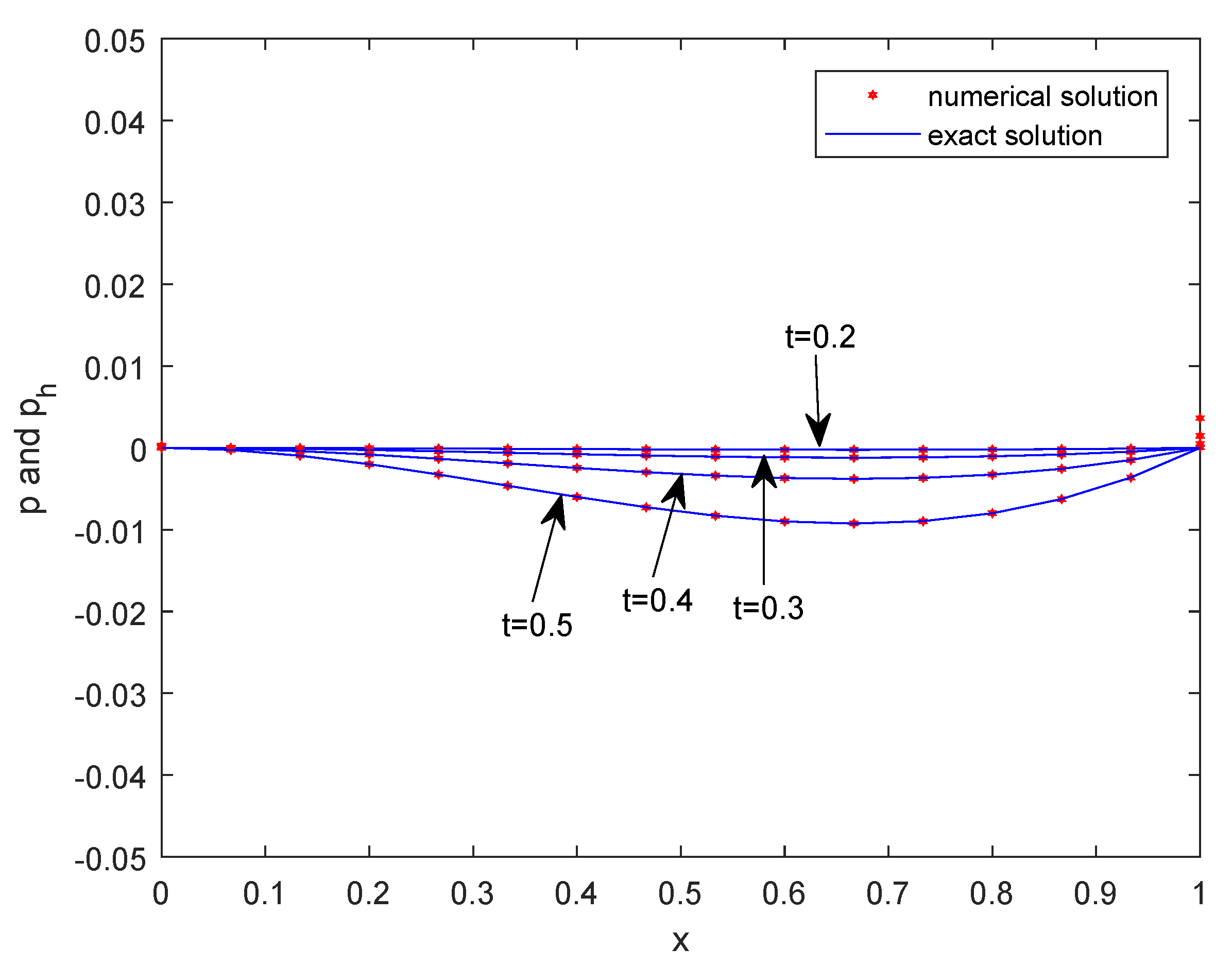
5. Numerical Example

In this section, we consider a numerical example in space–time domain $[0,1]\times [0,\frac{1}{2}]$ to verify the theoretical results of the $H^1$-Galerkin mixed finite element method. We choose $\omega \left(\alpha \right)=\Gamma (5-\alpha )$ in this numerical test. By choosing the nonlinear term $m\left(p\right)=sin\left(p\right)$, and the exact solution $p=t^4{x}^2(x-1)$, $u=t^4(3x^2-2x)$, we obtain the source term

$$f(x,t)=4t^3{x}^2(x-1)+\frac{24t^3(t-1)}{ln\left(t\right)}{x}^2(x-1)-t^4(6x-2)-4t^3(6x-2)+sin\left(t^4{x}^2(x-1)\right).$$

(73)

Here, for showing the feasibility and validity of our numerical method, we consider a linear element and provide the computing result by the Matlab procedure. In Table 1, with $\Delta \alpha =\frac{1}{500}$, $h=\frac{1}{500}$ and changed $\Delta t=\frac{1}{10},\frac{1}{20},\frac{1}{40}$, the errors and approximating second-order convergence rates in time are obtained, which are in agreement with the theoretical results. In Table 2, we obtain the distributed-order convergence results under the case $\Delta t^2\approx h^2\approx \Delta {\alpha }^4$. In Table 3, we show the errors and approximating second-order spatial convergence rates with $\Delta t=\frac{1}{500}$, $\Delta \alpha =\frac{1}{500}$ and changed $h=\frac{1}{10},\frac{1}{20},\frac{1}{40}$, which tell one that the results are in agreement with the case based on the linear element. Furthermore, the comparison between the numerical solution $p_h$ and the exact solution p at time $t=0.2,0.3,0.4,0.5$ with $\Delta t=\frac{1}{100}$, $\Delta \alpha =\frac{1}{8}$ and $h=\frac{1}{15}$ is made in Figure 1. Similarly, in Figure 2, the comparison between the exact solution u and the numerical solution $u_h$ is also shown based on the same discrete parameters as shown in Figure 1.

References

1. Feng, L.B.; Zhuang, P.; Liu, F.; Turner, I.; Gu, Y.T. Finite element method for space-time fractional diffusion equation. Numer. Algor. 2016, 72, 749–767. [Google Scholar] [CrossRef] [Green Version]
2. Zhao, M.; Cheng, A.J.; Wang, H. A preconditioned fast Hermite finite element method for space-fractional diffusion equations. Discrete Contin. Dyn. Syst.-Ser. B 2017, 22, 3529–3545. [Google Scholar] [CrossRef] [Green Version]
3. Zayernouri, M.; Karniadakis, G.E. Discontinuous spectral element methods for time-and space-fractional advection equations. SIAM J. Sci. Comput. 2014, 36, B684–B707. [Google Scholar] [CrossRef]
4. Yuste, S.B.; Quintana-Murillo, J. A finite difference method with non-uniform time steps for fractional diffusion equations. Comput. Phys. Commun. 2012, 183, 2594–2600. [Google Scholar] [CrossRef] [Green Version]
5. Yin, B.L.; Liu, Y.; Li, H. A class of shifted high-order numerical methods for the fractional mobile/immobile transport equations. Appl. Math. Comput. 2020, 368, 124799. [Google Scholar] [CrossRef]
6. Zeng, F.; Li, C.; Liu, F.; Turner, I. The use of finite difference/element approaches for solving the time-fractional subdiffusion equation. SIAM J. Sci. Comput. 2013, 35, A2976–A3000. [Google Scholar] [CrossRef]
7. Liu, Y.; Du, Y.W.; Li, H.; He, S.; Gao, W. Finite difference/finite element method for a nonlinear time-fractional fourth-order reaction-diffusion problem. Comput. Math. Appl. 2015, 70, 573–591. [Google Scholar] [CrossRef]
8. Liu, Y.; Du, Y.W.; Li, H.; Liu, J.C.; He, S. A two-grid mixed finite element method for a nonlinear fourth-order reaction-diffusion problem with time-fractional derivative. Comput. Math. Appl. 2015, 70, 2474–2492. [Google Scholar] [CrossRef]
9. Li, C.P.; Ding, H.F. Higher order finite difference method for the reaction and anomalous-diffusion equation. Appl. Math. Model. 2014, 38, 3802–3821. [Google Scholar] [CrossRef]
10. Lin, Y.M.; Xu, C.J. Finite difference/spectral approximations for the time fractional diffusion equation. J. Comput. Phys. 2007, 225, 1533–1552. [Google Scholar] [CrossRef]
11. Liu, Y.; Zhang, M.; Li, H.; Li, J.C. High-order local discontinuous Galerkin method combined with WSGD-approximation for a fractional subdiffusion equation. Comput. Math. Appl. 2017, 73, 1298–1314. [Google Scholar] [CrossRef] [Green Version]
12. Donatelli, M.; Mazza, M.; Serra-Capizzano, S. Spectral analysis and structure preserving preconditioners for fractional diffusion equation. J. Comput. Phys. 2016, 307, 262–279. [Google Scholar] [CrossRef]
13. Lin, X.L.; Ng, M.K.; Sun, H.W. A multigrid method for linear systems arising from time-dependent two-dimensional space-fractional diffusion equations. J. Comput. Phys. 2017, 336, 69–86. [Google Scholar] [CrossRef]
14. Bu, W.; Liu, X.; Tang, Y.; Jiang, Y. Finite element multigrid method for multi-term time fractional advection-diffusion equations. Int. J. Model. Simulat. Sci. Comput. 2015, 6, 1540001. [Google Scholar] [CrossRef]
15. Bu, W.P.; Tang, Y.F.; Yang, J.Y. Galerkin finite element method for two-dimensional Riesz space fractional diffusion equations. J. Comput. Phys. 2014, 276, 26–38. [Google Scholar] [CrossRef]
16. Jin, B.; Lazarov, R.; Liu, Y.K.; Zhou, Z. The Galerkin finite element method for a multi-term time-fractional diffusion equation. J. Comput. Phys. 2015, 281, 825–843. [Google Scholar] [CrossRef] [Green Version]
17. Yang, X.H.; Zhang, H.X.; Xu, D. Orthogonal spline collocation method for the two-dimensional fractional sub-diffusion equation. J. Comput. Phys. 2014, 256, 824–837. [Google Scholar] [CrossRef]
18. Wang, J.F.; Zhang, M.; Li, H.; Liu, Y. Finite difference/H1-Galerkin MFE procedure for a fractional water wave model. J. App. Anal. Comput. 2016, 6, 409–428. [Google Scholar]
19. Liu, Y.; Yu, Z.D.; Li, H.; Liu, F.W.; Wang, J.F. Time two-mesh algorithm combined with finite element method for time fractional water wave model. Int. J. Heat Mass Transfer 2018, 120, 1132–1145. [Google Scholar] [CrossRef]
20. Atangana, A. On the stability and convergence of the time-fractional variable order telegraph equation. J. Comput. Phys. 2015, 293, 104–114. [Google Scholar] [CrossRef]
21. Liu, Y.; Du, Y.W.; Li, H.; Liu, F.W.; Wang, Y.J. Some second-order θ schemes combined with finite element method for nonlinear fractional Cable equation. Numer. Algor. 2019, 80, 533–555. [Google Scholar] [CrossRef] [Green Version]
22. Wang, Y.J.; Liu, Y.; Li, H.; Wang, J.F. Finite element method combined with second-order time discrete scheme for nonlinear fractional Cable equation. Eur. Phys. J. Plus. 2016, 131, 61. [Google Scholar] [CrossRef]
23. Rebenda, J.; Smarda, Z. Numerical solution of fractional control problems via fractional differential transformation. In Proceedings of the European Conference on Electrical Engineering and Computer Science (EECS), Bern, Switzerland, 17–19 November 2017. [Google Scholar] [CrossRef] [Green Version]
24. Mainardi, F.; Pagnini, G.; Gorenflo, R. Some aspects of fractional diffusion equations of single and distributed order. Appl. Math. Comput. 2007, 187, 295–305. [Google Scholar] [CrossRef] [Green Version]
25. Diethelm, K.; Ford, N.J. Numerical analysis for distributed-order differential equations. J. Comput. Appl. Math. 2009, 225, 96–104. [Google Scholar] [CrossRef] [Green Version]
26. Ford, N.J.; Morgado, M.L.; Rebelo, M. An implicit finite difference approximation for the solution of the diffusion equation with distributed order in time. Electron. Trans. Numer. Anal. 2015, 44, 289–305. [Google Scholar]
27. Ye, H.; Liu, F.; Anh, V. Compact difference scheme for distributed-order time-fractional diffusion-wave equation on bounded domains. J. Comput. Phys. 2015, 298, 652–660. [Google Scholar] [CrossRef] [Green Version]
28. Meerschaert, M.M.; Nane, E.; Vellaisamy, P. Distributed-order fractional diffusions on bounded domains. J. Math. Anal. Appl. 2011, 379, 216–228. [Google Scholar] [CrossRef] [Green Version]
29. Luchko, Y. Boundary value problems for the generalized time-fractional diffusion equation of distributed order. Fract. Calc. Appl. Anal. 2009, 12, 409–422. [Google Scholar]
30. Gao, G.H.; Alikhanov, A.A.; Sun, Z.Z. The temporal second order difference schemes based on the interpolation approximation for solving the time multi-term and distributed-order fractional sub-diffusion equations. J. Sci. Comput. 2017, 73, 93–121. [Google Scholar] [CrossRef]
31. Lorenzo, C.F.; Hartley, T.T. Variable order and distributed order fractional operators. Nonlinear Dyn. 2002, 29, 57–98. [Google Scholar] [CrossRef]
32. Li, J.; Liu, F.; Feng, L.; Turner, I. A novel finite volume method for the Riesz space distributed-order diffusion equation. Comput. Math. Appl. 2017, 74, 772–783. [Google Scholar] [CrossRef]
33. Alikhanov, A.A. A new difference scheme for the time fractional diffusion equation. J. Comput. Phys. 2015, 280, 424–438. [Google Scholar] [CrossRef] [Green Version]
34. Li, X.L.; Rui, H.X. Two temporal second-order H1-Galerkin mixed finite element schemes for distributed-order fractional sub-diffusion equations. Numer. Algor. 2018, 79, 1107–1130. [Google Scholar] [CrossRef]
35. Abbaszadeh, M.; Dehghan, M. An improved meshless method for solving two-dimensional distributed order time-fractional diffusion-wave equation with error estimate. Numer. Algor. 2017, 75, 173–211. [Google Scholar] [CrossRef]
36. Liu, Y.; Du, Y.W.; Li, H.; Wang, J.F. An H1-Galerkin mixed finite element method for time fractional reaction-diffusion equation. J. Appl. Math. Comput. 2015, 47, 103–117. [Google Scholar] [CrossRef]
37. Pani, A.K. An H1-Galerkin mixed finite element methods for parabolic partial differential equations. SIAM J. Numer. Anal. 1998, 35, 712–727. [Google Scholar] [CrossRef]
38. Liu, Y.; Li, H. H1-Galerkin mixed finite element methods for pseudo-hyperbolic equations. Appl. Math. Comput. 2009, 212, 446–457. [Google Scholar]
39. Guo, L.; Chen, H. H1-Galerkin mixed finite element method for the regularized long wave equation. Computing 2006, 77, 205–221. [Google Scholar] [CrossRef]
40. Wang, J.F.; Liu, T.Q.; Li, H.; Liu, Y.; He, S. Second-order approximation scheme combined with H1-Galerkin MFE method for nonlinear time fractional convection-diffusion equation. Comput. Math. Appl. 2017, 73, 1182–1196. [Google Scholar] [CrossRef]
41. Shi, Z.G.; Zhao, Y.M.; Liu, F.; Tang, Y.F.; Wang, F.L.; Shi, Y.H. High accuary analysis of an H1-Galerkin mixed finite element method for two-dimensional time fractional diffusion equations. Comput. Math. Appl. 2017, 74, 1903–1914. [Google Scholar] [CrossRef]
42. Shi, D.Y.; Wang, J.J.; Yan, F.N. Unconditional superconvergence analysis of an H1-Galerkin mixed finite element method for nonlinear Sobolev equations. Numer. Meth. Part. Differ. Equ. 2018, 34, 145–166. [Google Scholar] [CrossRef]
43. Sun, H.; Sun, Z.Z.; Gao, G.H. Some temporal second order difference schemes for fractional wave equations. Numer. Meth. Part Differ. Equ. 2016, 32, 970–1001. [Google Scholar] [CrossRef]
Figure 1. Comparison between p and p h at time t = 0.2 , 0.3 , 0.4 , 0.5 .
Mathematics 08 00187 g001
Figure 2. Comparison between u and u h at time t = 0.2 , 0.3 , 0.4 , 0.5 .
Mathematics 08 00187 g002