Asymptotically Convergent Higher-Order Switching Differentiator

Abstract

A novel switching-differentiator (SD) that can asymptotically track the time derivative of time-varying signal was previously proposed. This paper extends the previous SD to estimation of higher-order time derivatives. This study shows that higher-order time-derivatives can be estimated by connecting multiple SDs in cascade form. By successive applying the generalized Barbalat’s lemma, all higher-order tracking errors also approach zeros asymptotically. To illustrate the performance of the proposed higher-order switching differentiator, simulations were performed for estimating higher-order time-derivatives of a signal.

1. Introduction

In the field of controllers for linear or nonlinear systems, the online time-derivative estimator or differentiator plays a crucial role. Applications of differentiators include proportional–integral–derivative (PID) controller [1,2], state estimator in the output-feedback controller [3,4,5], active disturbance rejection [1,6], fault diagnosis schemes [7], and approximation-free controller for uncertain nonlinear systems [8,9,10]. The performance of the controller is directly influenced by that of the differentiator. Therefore, extensive research studies have been performed on differentiators, including high-order sliding mode differentiators (HOSMDs) [4,11,12,13], singular perturbation-technique-based differentiators [14], high-gain observers (HGOs) [3,15,16], uniformly convergent differentiators [17], and augmented nonlinear differentiators [18]. Especially in the output-feedback controller design of uncertain nonlinear systems, HGO and HOSMD are widely adopted differentiators. The HGO dynamics has a relatively simple linear form. It has a drawback of peaking caused by a non-zero initial condition. Thus, it is not robust against measurement noise. The HOSMD has the advantages of finite-time exact convergence and robustness against disturbance. However, HOSMD contains switching functions in its dynamics, so its estimations inevitably contain chatterings. Another drawback of HOSMD is that its dynamic equations are rather complex.

Park et al. proposed a novel switching-differentiator (SD) that can asymptotically track the time-derivative of a signal in [19]. Its dynamic equation has a simple form and neither peaking nor chattering occur in the estimation. Another merit of this SD is that the tracking error tends to be zero asymptotically irrespective of the large initial error. In addition, it is robust against measurement disturbance. However, in [19], the SD was geometrically proved only for the first-order time-derivative estimation case. In this study, the SD was extended to the case of higher-order time-derivative estimations. We prove that higher-order time-derivatives can be observed by connecting multiple SDs in cascade and that tracking errors can go to zero asymptotically by successive applying the generalized Barbalat’s lemma [20]. The merits of the proposed higher-order switching differentiator (HOSD) are summarized as follows:

• The proposed HOSD can estimate higher-order time-derivatives of a time-varying signal. Estimation errors are proved to approach zero asymptotically irrespective of large initial errors.
• The HOSD estimations show no peaking or chattering, although its dynamics contain switching functions.
• The dynamic equations and structure of the differentiator are relatively simple compared with those of other well-known derivative estimators.

We compared the performance of HGO, HOSMD and the proposed HOSD via simulations. Simulations of the estimations of higher-order time-derivatives of a signal were conducted to compare and illustrate the performance of the proposed HOSD.

2. Main Results

2.1. Preliminaries

Definitions of $\mathbb{N}=\{1,2,\cdots \}$, ${\mathbb{N}}_0=\{0,1,2,\cdots \}$, and ${\mathbb{R}}_0^{+}=\left\{0\right\}\cup {\mathbb{R}}^{+}$ are used throughout this paper. Denotation $a\left(t\right)\to b$ is an abbreviated expression of ${lim}_{t\to \infty }a\left(t\right)=b$. The following definitions are also used throughout this paper:

Definition 1.

Let Φ be a set of all strictly increasing infinite sequences whose first numbers are zeros such that:

$$\begin{array}{c}\hfill \mathsf{\Phi }\triangleq \left\{{\left(t_i\right)}_{i=0}^{\infty }\right|t_0=0,t_i<t_{i+1}\forall i\in {\mathbb{N}}_0\}.\end{array}$$

(1)

Definition 2.

For a sequence $T=\left(t_i\right)\in \mathsf{\Phi }$, let $f\left(t\right):{\mathbb{R}}_0^{+}\to \mathbb{R}$ be a continuous function, that is, $f\left(t\right)$ is not disconnected at any $t=t_i$. Let $g\left(t\right):{\mathbb{R}}_0^{+}\to \mathbb{R}$ be a piecewise continuous function disconnected at some or all $t_i$. The set of all f and g is denoted ${\mathsf{\Omega }}_T$.

Definition 3.

For $T=\left(t_i\right)\in \mathsf{\Phi }$, define the set of functions as follows:

$${\overline{\mathsf{\Omega }}}_T^L\triangleq \left\{f\left(t\right)|f\left(t\right)\in {\mathsf{\Omega }}_T,\underset{\begin{array}{c}{t}_i\le t<t_{i+1}\\ \forall i\in {\mathbb{N}}_0\end{array}}{sup}\left|f\left(t\right)\right|\le L<\infty \right\}$$

(2)

where $L>0$ is a constant. The functions in ${\overline{\mathsf{\Omega }}}_T^L$ refer to be bounded in the piecewise sense (BPWS) below L.

If a continuous function f is in ${\overline{\mathsf{\Omega }}}_T^L$, f is simply a bounded continuous function, i.e., $\left|f\left(t\right)\right|\le L$ for $t\ge 0$.

Fact 1.

Consider two functions $f\in {\overline{\mathsf{\Omega }}}_{T_f}^{L_f}$ and $g\in {\overline{\mathsf{\Omega }}}_{T_g}^{L_g}$, where $T_f,T_g\in \mathsf{\Phi }$. Then $f+g$ is bounded in the piececwise sense, that is, $f+g\in {\overline{\mathsf{\Omega }}}_T^L$ with $T\triangleq T_f\cup T_g$ and $L\triangleq L_f+L_g$.

The proof of Fact 1 is trivial. Thus, it is omitted.

In [20], the following more generalized version of the conventional Barbalat’s lemma was presented as follows:

Lemma 1.

Let $T=\left(t_i\right)\in \mathsf{\Phi }$. Suppose $V\left(t\right):{\mathbb{R}}_0^{+}\to \mathbb{R}$ satisfies:

1. 

${lim}_{t\to \infty }$V(t) exists.

2. 

$V\left(t\right)$ is twice differentiable on each interval $[t_i,t_{i+1})$.

3. 

$L>0$ exists, such that $\ddot{V}\in {\overline{\mathsf{\Omega }}}_T^L$.

Then $\dot{V}\left(t\right)\to 0$.

According to ([20] Remark 1), because V and $\dot{V}$ can be piececewise functions, Lemma 1 can be regarded as an extension of the conventional Barbarlat’s lemma to the class of piecewise continuous functions by requiring $\ddot{V}$ to be bounded in the piecewise sense.

Park et al. proposed an asymptotically convergent firstst-order time-derivative estimator in [19]. The main result of [19] can be described as follows.

Lemma 2.

Consider the following dynamics, where $a\left(t\right)$ is the time-varying signal that satisfies $|\ddot{a}\left(t\right)|\le L_1^{*}<\infty$ for all $t\ge 0$

$$\begin{array}{ccc}\hfill \dot{{\alpha }_1}& =& k_1{e}_{{\alpha }_1}+{\sigma }_1\hfill \end{array}$$

(3)

$$\begin{array}{ccc}\hfill \dot{{\sigma }_1}& =& L_1\mathrm{sgn}\left(e_{{\alpha }_1}\right)\hfill \end{array}$$

(4)

where $e_{{\alpha }_1}\triangleq a-{\alpha }_1$. Then, ${\sigma }_1$ in (4) is asymptotically convergent to $\dot{a}$ if $L_1>L_1^{*}$ and $k_1>0$.

Here, $\mathrm{sgn}(·)$ is a switching function defined as follows:

$$\mathrm{sgn}\left(e_{\alpha }\right)=\left\{\begin{array}{cc}1,\hfill & e_{\alpha }\ge 0\hfill \\ -1,\hfill & e_{\alpha }<0\hfill \end{array}\right.$$

(5)

Note that in Lemma 2, $\ddot{a}$ is allowed to be the piecewise continuous function as long as it is bounded. That is, the property of Lemma 2 still holds for $\ddot{a}\in {\overline{\mathsf{\Omega }}}_{T_a}^{L^{*}}$ where $T_a\in \mathsf{\Phi }$. As commented above, in [19], Park et al. proved that ${\sigma }_1$ approaches $\dot{a}$ asymptotically. That is, denoting the estimation error as:

$$e_{{\sigma }_1}=\dot{a}-{\sigma }_1$$

(6)

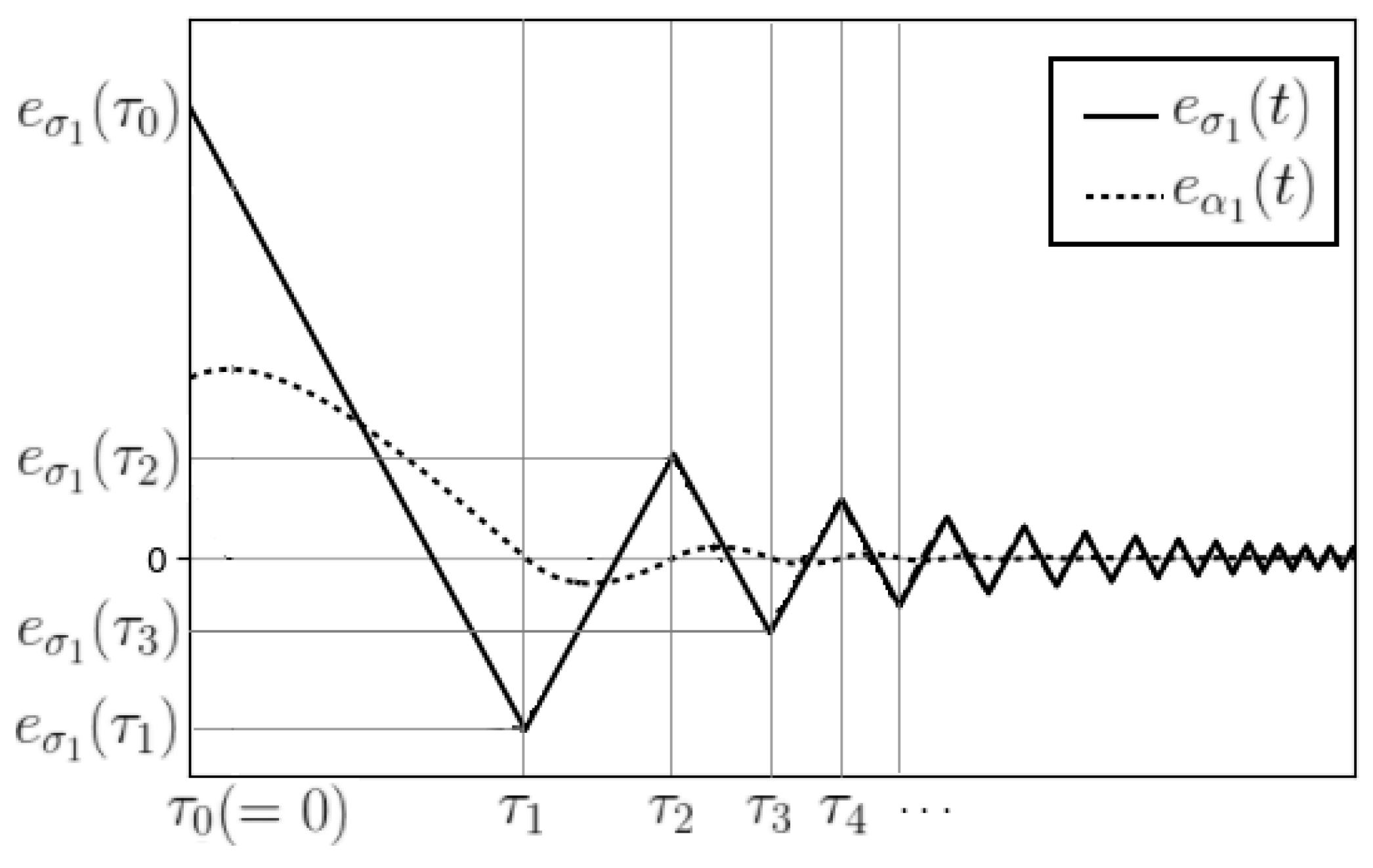
Then, Lemma 2 describes $e_{{\sigma }_1}\left(t\right)\to 0$. For a description of the more specific behavior of $e_{{\sigma }_1}$, which is required in the proof process of the following Lemmas, define infinite time sequence $T_{{\sigma }_1}\triangleq \left({\tau }_i\right)\in \mathsf{\Phi }$, where $\mathrm{sgn}\left(e_{{\alpha }_1}(t={\tau }_i)\right)$ changes its value (from 1 to −1 or vice versa). In [19], Park et al. showed that an infinite number of time intervals exists $[{\tau }_i,{\tau }_{i+1})$, such that ${lim}_{i\to \infty }({\tau }_{i+1}-{\tau }_i)=0$. The $e_{{\sigma }_1}$ changes its sign (i.e., $e_{{\sigma }_1}$ crosses the $e_{{\sigma }_1}=0$ line) at some time point $t\in ({\tau }_i,{\tau }_{i+1})$. The fact that inequality $|e_{{\sigma }_1}\left({\tau }_{i+1}\right)|<|e_{{\sigma }_1}\left({\tau }_i\right)|$ holds for all $i\in \mathbb{N}$, as also been proven in [19]. The typical trajectory of $e_{{\sigma }_1}$ is illustrated in Figure 1. As shown in Figure 1, $e_{{\sigma }_1}\left(t\right)$ oscillates and its magnitude converges to zero asymptotically.

Figure 1. Typical trajectory of $e_{{\sigma }_1}\left(t\right)$ (solid line) and $e_{{\alpha }_1}\left(t\right)$ (dotted line).

2.2. Expansion to the Second-Order Differentiator

The first concern for the next step in the higher-order expansion is the behavior of $e_{{\sigma }_1}^{\left(i\right)}$ for $i\in \mathbb{N}$, whose dynamics are described as:

$$e_{{\sigma }_1}^{\left(i\right)}=a^{(i+1)}-{\sigma }_1^{\left(i\right)}$$

(7)

To prove convergence of $e_{{\sigma }_1}^{\left(i\right)}$, the conventional Barbalat’s lemma cannot be applied since the $e_{{\sigma }_1}^{\left(i\right)}$ has a piecewise continuous function. By using Lemma 1 instead of Barbalat’s lemma, the following key aspects can be directly proven:

Fact 2.

If $a^{(j+2)}\in {\overline{\mathsf{\Omega }}}_{T_a}^{L_{j+1}^{*}}$ for all $j=0,1,\cdots ,i+1$ where $L_{j+1}^{*}>0$ and $T_a\in \mathsf{\Phi }$, then $e_{{\sigma }_1}^{\left(i\right)}\to 0$ for all $i\in \mathbb{N}$.

Proof. 

In the case of $i=1$, if we let $V_0\triangleq e_{{\sigma }_1}$, then condition (1) of Lemma 1 is satisfied since $V_0\to 0$ by Lemma 2. Because both $\dot{a}$ and ${\sigma }_1$ have piecewise continuous functions, $V_0(=e_{{\sigma }_1})$ is twice differentiable in the piecewise sense. Considering ${\ddot{V}}_0=\stackrel{⃛}{a}-{\ddot{\sigma }}_1$, since $a^{\left(3\right)}\in {\overline{\mathsf{\Omega }}}_{T_a}^{L_2^{*}}$ holds by assumption and ${\ddot{\sigma }}_1={\overline{\mathsf{\Omega }}}_{T_{{\sigma }_1}}^0$ by (4), it can be concluded that ${\ddot{V}}_0\in {\overline{\mathsf{\Omega }}}_{T_a\cup T_{{\sigma }_1}}^{L_2^{*}}$ from Fact 1. Thus, conditions (2) and (3) of Lemma 1 are also satisfied for $V_0$, which results in ${\dot{V}}_0\left(t\right)={\dot{e}}_{{\sigma }_1}\left(t\right)\to 0$.

Next, let us define $V_i\triangleq e_{{\sigma }_1}^{\left(i\right)}$. Using mathematical induction, it is sufficient to show that $V_{i+1}\left(t\right)\to 0$ holds under the assumption of $V_i\left(t\right)\to 0$. $V_i$ is twice differentiable in the piecewise sense and we obtain ${\ddot{V}}_i=a^{(i+3)}-{\sigma }_1^{(i+2)}$. Since $a^{(i+3)}\in {\overline{\mathsf{\Omega }}}_{T_a}^{L_{i+2}^{*}}$ and ${\sigma }_1^{(i+2)}\in {\overline{\mathsf{\Omega }}}_{T_{{\sigma }_1}}^0$ hold, $\ddot{V_i}$ is also in ${\overline{\mathsf{\Omega }}}_{T_a\cup T_{{\sigma }_1}}^{L_{i+2}^{*}}$ by Fact 1. Because all conditions in Lemma 1 are met, it can be concluded that $\dot{V_i}=V_{i+1}\to 0$. This completes the proof. □

Using Lemma 2 and Fact 2, an asymptotically convergent second-order time-derivative estimator can be constructed by connecting two SDs in a cascade form.

Lemma 3.

Assume a signal $a\left(t\right)$ satisfies $\ddot{a}\left(t\right)\in {\overline{\mathsf{\Omega }}}_T^{L_1^{*}}$, $\stackrel{⃛}{a}\left(t\right)\in {\overline{\mathsf{\Omega }}}_T^{L_2^{*}}$ for some positive constants $L_1^{*}$, $L_2^{*}$, and $T\in \mathsf{\Phi }$. $a^{\left(4\right)}$ is also assumed to be bounded in the piecewise sense. Consider the following dynamics:

$$\begin{array}{c}\hfill \begin{array}{cc}{\dot{\alpha }}_1& =k_1{e}_{{\alpha }_1}+{\sigma }_1\hfill \\ {\dot{\sigma }}_1& =L_1\mathrm{sgn}\left(e_{{\alpha }_1}\right)\hfill \end{array}\}\end{array}$$

(8)

$$\begin{array}{c}\hfill \begin{array}{cc}{\dot{\alpha }}_2& =k_2{e}_{{\alpha }_2}+{\sigma }_2\hfill \\ {\dot{\sigma }}_2& =L_2\mathrm{sgn}\left(e_{{\alpha }_2}\right)\hfill \end{array}\}\end{array}$$

(9)

where $e_{{\alpha }_1}=a-{\alpha }_1$ and $e_{{\alpha }_2}={\sigma }_1-{\alpha }_2$. If $L_1>L_1^{*}$, $k_1>0$, $L_2>L_2^{*}$, and $k_2>0$, then ${\sigma }_1\left(t\right)\to \dot{a}$ and ${\sigma }_2\left(t\right)\to \ddot{a}$.

Proof. 

From Lemma 2, by defining $e_{{\sigma }_1}\triangleq \dot{a}-{\sigma }_1\left(t\right)$, the estimate of $\dot{a}$ is:

$${\sigma }_1\left(t\right)=\dot{a}-e_{\sigma 1}$$

(10)

with $e_{{\sigma }_1}\left(t\right)\to 0$. In the second SD (9), ${\sigma }_2$ is the estimate of $\dot{{\sigma }_1}$. From Fact 2, ${\ddot{e}}_{{\sigma }_1}\left(t\right)\to 0$ holds, which means ${\ddot{\sigma }}_1\left(t\right)\to \stackrel{⃛}{a}$. Therefore, $t_{c1}$ exists, such that $|{\ddot{\sigma }}_1|\le L_2^{*}$ for $t\ge t_{c1}$. If we let $e_{{\sigma }_2}\triangleq {\dot{\sigma }}_1-{\sigma }_2\left(t\right)$, then:

$${\sigma }_2\left(t\right)={\dot{\sigma }}_1-e_{{\sigma }_2}.$$

(11)

After $t_{c1}$, $e_{{\sigma }_2}\left(t\right)\to 0$ is also guaranteed again from Lemma 2, substituting (10) into (11) results in:

$${\sigma }_2\left(t\right)=\ddot{a}-{\dot{e}}_{{\sigma }_1}-e_{{\sigma }_2}.$$

(12)

From Fact 2, ${\dot{e}}_{{\sigma }_1}\left(t\right)\to 0$ is satisfied. Thus, it can be concluded that ${\sigma }_2\left(t\right)\to \ddot{a}$. □

Fact 3.

For $i\in \mathbb{N}$, $e_{{\sigma }_2}^{\left(i\right)}\left(t\right)\to 0$ holds.

Proof. 

We already proved in Lemma 3 that $e_{{\sigma }_2}\left(t\right)\to 0$ holds. From the definition of $e_{{\sigma }_2}^{\left(i\right)}\triangleq {\sigma }_1^{(i+1)}-{\sigma }_2^{\left(i\right)}$ and ${\sigma }_1^{(i+1)}\in {\overline{\mathsf{\Omega }}}_{T_{{\sigma }_1}}^0$, ${\sigma }_2^{\left(i\right)}\in {\overline{\mathsf{\Omega }}}_{T_{{\sigma }_2}}^0$ for $i\in \mathbb{N}$, it can be concluded that $e_{{\sigma }_2}^{\left(i\right)}$ is also in ${\overline{\mathsf{\Omega }}}_{T_{{\sigma }_1}\cup T_{{\sigma }_2}}^0$ for $i\in \mathbb{N}$. By repeatedly applying Lemma 1, it can be recursively guaranteed that $e_{{\sigma }_2}^{\left(i\right)}\left(t\right)\to 0$ via mathematical induction. □

2.3. Expansion to HOSD

Using the preliminary facts and second-order differentiator, the SD can be extended to the HOSD with asymptotically convergent estimations. The main result in this paper is described in the following theorem.

Theorem 1.

Let $i\in N$, and for a signal $a\left(t\right)$, assume that $a^{(j+1)}\in {\overline{\mathsf{\Omega }}}_T^{L_j^{*}}$ for $j=1,2,\cdots ,i$ where $L_j^{*}$’s are positive constants and $T\in \mathsf{\Phi }$. $a^{(i+2)}$ is assumed to be bounded in the piecewise sense. Consider the following HOSD dynamics:

$$\begin{array}{c}\hfill \begin{array}{cc}{\dot{\alpha }}_j& =k_j{e}_{{\alpha }_j}+{\sigma }_j,\hfill \\ {\dot{\sigma }}_j& =L_j\mathrm{sgn}\left(e_{{\alpha }_j}\right)\hfill \end{array}\},j=1,2,\cdots ,i\end{array}$$

(13)

where $e_{{\alpha }_j}={\sigma }_{j-1}-{\alpha }_j$ with ${\sigma }_0=a$. If the design constants are chosen such that $k_j>0$ and $L_j>L_j^{*}$ for all $j=1,2,\cdots ,i$, then:

$${\sigma }_j\left(t\right)\to a^{\left(j\right)},j=1,2,\cdots ,i$$

(14)

holds.

Proof. 

For convenience, Equations (10) and (12) in Lemma 3 are rewritten here as follows:

$$\begin{array}{ccc}\hfill {\sigma }_1\left(t\right)& =& \dot{a}-e_{\sigma 1}\hfill \end{array}$$

(15)

$$\begin{array}{ccc}\hfill {\sigma }_2\left(t\right)& =& \ddot{a}-{\dot{e}}_{{\sigma }_1}-e_{{\sigma }_2}\hfill \end{array}$$

(16)

Since, ${\ddot{e}}_{{\sigma }_2}\to 0$ holds from Fact 3, which means ${\ddot{\sigma }}_2\to {\stackrel{⃛}{\sigma }}_1\to a^{\left(4\right)}$, $t_{c2}$ exists, such that $|{\ddot{\sigma }}_2|\le L_3^{*}$ for $t>t_{c2}$. By defining $e_{{\sigma }_3}={\dot{\sigma }}_2-{\sigma }_3$, ${\sigma }_3$ can be written using (16) as:

$$\begin{array}{ccc}{\sigma }_3\left(t\right)& =& {\dot{\sigma }}_2-e_{{\sigma }_3}\hfill \\ & =& \stackrel{⃛}{a}-{\ddot{e}}_{{\sigma }_1}-{\dot{e}}_{{\sigma }_2}-e_{{\sigma }_3}\hfill \end{array}$$

(17)

with $e_{{\sigma }_3}\to 0$ after $t_{c2}$ by Lemma 2. In general, ${\sigma }_j$ is recursively derived as:

$$\begin{array}{c}\hfill {\sigma }_j\left(t\right)=a^{\left(j\right)}-\sum _{k=0}^{j-1}{e}_{{\sigma }_{j-k}}^{\left(k\right)},j=1,\cdots ,i\end{array}$$

(18)

where $e_{{\sigma }_j}\triangleq {\dot{\sigma }}_{j-1}-{\sigma }_j$ with ${\sigma }_0=a$. The following is the procedure for the mathematical induction.

Assume that $e_{{\sigma }_{j-1}}^{\left(k\right)}\to 0$, $e_{{\sigma }_{j-2}}^{\left(k\right)}\to 0$, ⋯, $e_{{\sigma }_1}^{\left(k\right)}\to 0$ for all $k\in {\mathbb{N}}_0$. The fact ${\ddot{e}}_{{\sigma }_{j-1}}\left(t\right)\to 0$ implies ${\ddot{\sigma }}_{j-1}\to {\stackrel{⃛}{\sigma }}_{j-2}\to {\sigma }_{j-3}^{\left(4\right)}\to \cdots \to {\sigma }_1^{\left(j\right)}\to a^{(j+2)}$. Therefore, $t_{c_j}$ exists such that $|{\ddot{\sigma }}_{j-1}|\le L_{j+1}^{*}$ for $t>t_{c_j}$. Thus, $e_{{\sigma }_j}\to 0$ by Lemma 2 after $t_{c_j}$. It is true that all summed terms in the right-hand side of (18) tend to be zero, which leads to ${\sigma }_j\left(t\right)\to a^{\left(j\right)}$. The convergent property of $e_{{\sigma }_j}^{\left(k\right)}\to 0$ for $k\in \mathbb{N}$ can be easily performed by similar procedure of the proof of Fact 2 or Fact 3. Thus, it is omitted.

Combining all these together, it can be concluded that, for $k\in {\mathbb{N}}_0$:

• $e_{{\sigma }_1}^{\left(k\right)}\to 0$ holds
• $e_{{\sigma }_j}^{\left(k\right)}\to 0$ for $j=2,\cdots ,i$ holds under the assumptions of $e_{{\sigma }_m}^{\left(k\right)}\to 0$ for $m=1,2,\cdots ,j-1$.

Therefore, it can be recursively proven that (14) holds. □

Remark 1.

Through various simulations, we found that parameter $k_j$ must be chosen as a large enough value to ensure good performance. We recommend that $k_j$ is selected as tens to thousands of times $L_j$.

3. Simulation

3.1. Example 1

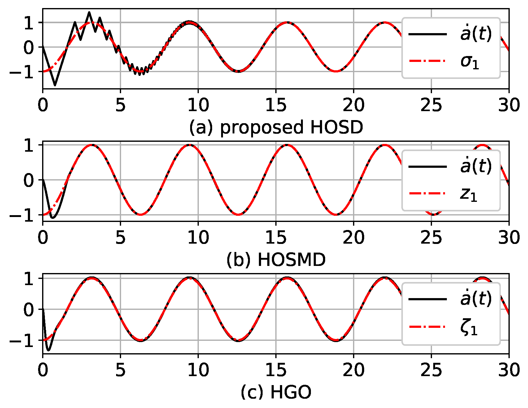
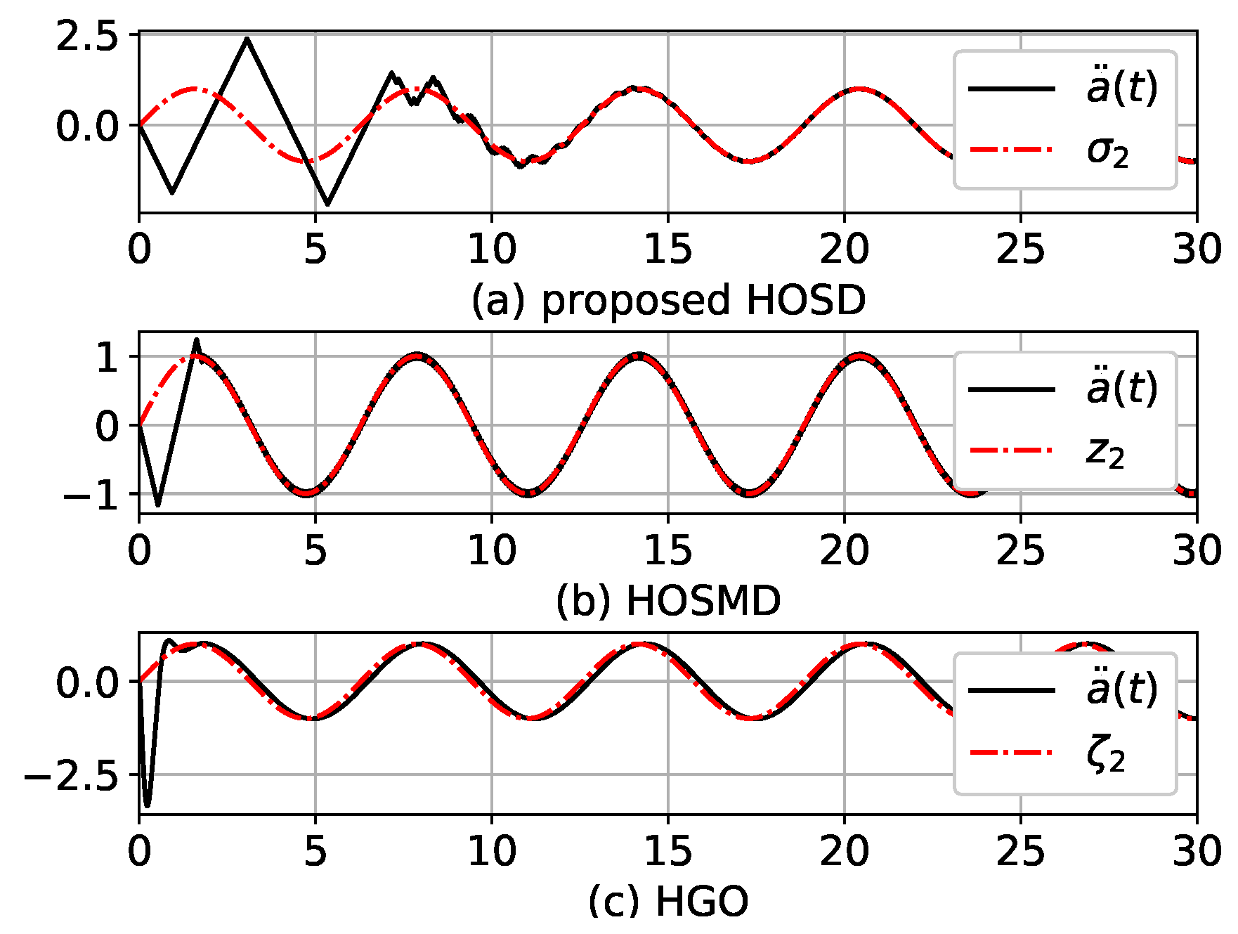
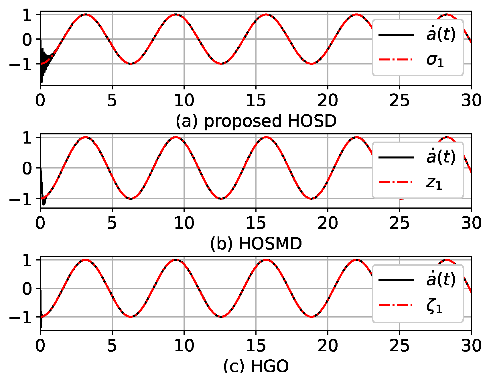
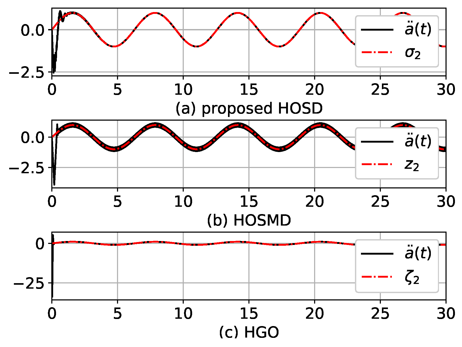
In this section, the performance of the proposed HOSD is shown via simulations. In the following simulations, Python language and its libraries, such as scipy, numpy, and matplotlib [21], are used. Time-derivatives of $a\left(t\right)=-sint$ are estimated by the proposed HOSD, HOSMD, and HGO. Estimations were also compared. Time-derivatives of $a\left(t\right)$ are $\dot{a}=-cost$ and $\ddot{a}=sint$. First, the proposed HOSD equations of (8) and (9) were used to estimate $\dot{a}$ and $\ddot{a}$. The HOSMD is a second estimator whose dynamics are as follows:

$$\begin{array}{ccc}\hfill {\dot{z}}_0& =& -3M^{\frac{1}{3}}{\lceil z_0-a\left(t\right)\rfloor }^{\frac{2}{3}}+z_1\triangleq v_0\hfill \end{array}$$

$$\begin{array}{ccc}\hfill {\dot{z}}_1& =& -1.5M^{\frac{1}{2}}{\lceil z_1-v_0\rfloor }^{\frac{1}{2}}+z_2\triangleq v_1\hfill \end{array}$$

$$\begin{array}{ccc}\hfill {\dot{z}}_2& =& -1.1M\mathrm{sgn}(z_2-v_1)\hfill \end{array}$$

(19)

where ${\lceil x\rfloor }^p={\left|x\right|}^p\mathrm{sgn}\left(x\right)$ and $M>0$ are positive design constants. In (19), $z_1$ and $z_2$ were used as estimates of $\dot{a}$ and $\ddot{a}$, respectively. The third one is the HGO, which has the following form:

$$\begin{array}{ccc}\hfill {\dot{\zeta }}_0& =& {\zeta }_1+(c_0/ϵ)(a\left(t\right)-{\zeta }_0)\hfill \end{array}$$

$$\begin{array}{ccc}\hfill {\dot{\zeta }}_1& =& {\zeta }_2+(c_1/{ϵ}^2)(a\left(t\right)-{\zeta }_0)\hfill \end{array}$$

$$\begin{array}{ccc}\hfill {\dot{\zeta }}_2& =& (c_2/{ϵ}^3)(a\left(t\right)-{\zeta }_0)\hfill \end{array}$$

(20)

where $c_i$’s ($i=0,1,2$) and $ϵ>0$ are design constants. The estimates of $\dot{a}$ and $\ddot{a}$ are ${\zeta }_1$ and ${\zeta }_2$, respectively. Three sets of parameters were chosen as presented in Table 1.

Table 1. Simulation parameter sets.

	HOSD	HOSDM	HGO
①	$k_1=k_2=1$	$M=2$	$c_0=3$, $c_1=2$
	$L_1=L_2=2$		$c_2=1$, $ϵ=0.1$
②	$k_1=k_2=10$	$M=20$	$c_0=3$, $c_1=2$
	$L_1=L_2=20$		$c_2=1$, $ϵ=0.01$
③	$k_1=k_2=10,000$	$M=2000$	$c_0=3$, $c_1=2$
	$L_1=L_2=2000$		$c_2=1$, $ϵ=0.001$

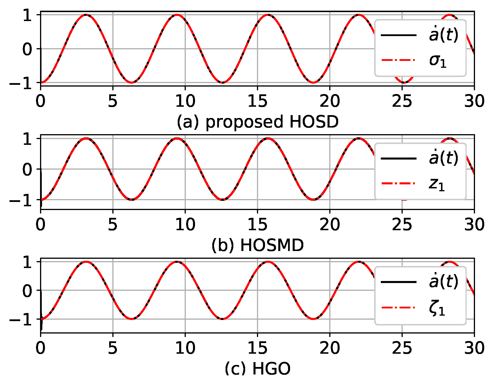
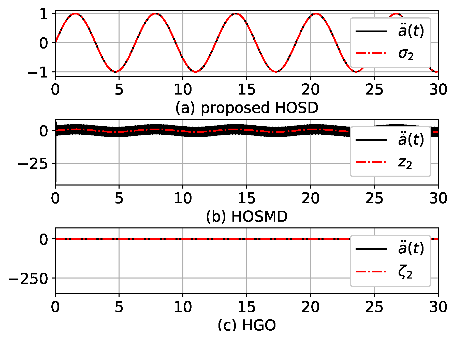
The simulation results using parameter set ① in Table 1 are depicted in Figure 2 and Figure 3. Since the gains are relatively small compared to those of other parameter sets, estimation errors move toward zero slowly. Although the tracking errors of HOSD and HOSMD also go to zero, HGO estimations had relatively larger peaking and steady-state errors, as shown in Figure 3c.

Figure 2. Estimations of $\dot{a}$ using parameter set ① in Table 1.

Figure 3. Estimations of $\ddot{a}$ using parameter set ① in Table 1.

Figure 4 and Figure 5 illustrate the simulation results using parameter set ② in Table 1. Due to sufficiently large gains, $\dot{a}$ and $\ddot{a}$ were exactly estimated by HOSD, HOSMD, and HGO. However, in the case of HOSMD, if M was larger to achieve a short transient time, chattering in the estimation appeared (Figure 5b). The HGO estimations showed considerably larger peaking at $t=0$ as shown in Figure 5c since the $ϵ$ value decreased.

Figure 4. Estimations of $\dot{a}$ using parameter set ② in Table 1.

Figure 5. Estimations of $\ddot{a}$ using parameter set ② in Table 1.

The parameter set ③ in Table 1 is stronger than those in sets ② and ①. Figure 6 and Figure 7 illustrate the results. In this case, the advantage of the proposed HOSD is even more pronounced. The estimations of HOSD seemed to be exact. No peaking or chattering were observed in ${\sigma }_1$ or ${\sigma }_2$ (Figure 6a and Figure 7a). However, in the estimation of HOSMD, peaking and chattering in $z_2$ existed as depicted in Figure 7b. In the case of HGO, huge peaking in ${\zeta }_2$ at $t=0$ appeared (Figure 7c).

Figure 6. Estimations of $\dot{a}$ using parameter set ③ in Table 1.

Figure 7. Estimations of $\ddot{a}$ using parameter set ③ in Table 1.

3.2. Example 2

In this section, the performance of differentiator-based controllers for an uncertain nonlinear system is compared. In [9], Park et al. proposed a HOSMD-based output-feedback controller for uncertain nonautonomous and nonaffine pure-feedback nonlinear systems. The HOSMD that was adopted in the controller of [9] was replaced by HOSD and HGO. The performance and properties of these three different controllers based on HOSMD, HGO, and the proposed HOSD were compared via simulations.

The dynamic equations of the example second-order pure-feedback nonlinear system are shown as follows:

$$\begin{array}{ccc}\hfill {\dot{x}}_1& =& 0.1x_{1}cos10t+(1+x_1^2)x_2\hfill \end{array}$$

(21)

$$\begin{array}{ccc}\hfill {\dot{x}}_2& =& x_1{x}_2+u+\frac{u^3}{7}+0.5sin5t\hfill \end{array}$$

(22)

where $x_1$ and u are the output and input of the system, respectively; $x_2$ is an unmeasurable state variable. Note that the controller has no information on the dynamic equations and contained disturbances. Due to the term $u^3/7$ in (22), this example system is sensitive to small changes in the control input, which complicates the control of the output. The control objective was to drive $y(=x_1)$ for tracking $y_d\left(t\right)$ while maintaining all signals as bounded.

The controller design procedure proposed in [9] is summarized as follows:

• Construct a differentiator that can estimate up to second time-derivatives of a signal $a\left(t\right)$, which is defined in the next step. Let ${\sigma }_1$ and ${\sigma }_2$ be the estimate of $\dot{a}$ and $\ddot{a}$, respectively, in what follows.
• The signal $a\left(t\right)$ is composed using the following control input filtering:

  $$\begin{array}{ccc}\hfill {\dot{w}}_1& =& -c{w}_1+w_2\hfill \end{array}$$

  $$\begin{array}{ccc}\hfill {\dot{w}}_2& =& -c{w}_2+u\hfill \end{array}$$

  $$\begin{array}{ccc}\hfill a& =& e-w_1\hfill \end{array}$$

  (23)

  where $c>0$ is a design constant usually chosen as 1, and $e=x_1-y_d$ is the tracking error.
• The control law is determined as:

  $$\begin{array}{c}\hfill u=-{\sigma }_2-p_2-{\mathbf{g}}^{\mathrm{T}}\widehat{\mathbf{e}}\end{array}$$

  (24)

  where $\mathbf{g}={[g_1,g_2]}^{\mathrm{T}}$ is a constant vector chosen such that the equation:

  $${(s+g)}^2=s^2+g_{2}s+g_1$$

  (25)

  holds with $g>0$. The estimate of tracking error vector is determined as:

  $$\begin{array}{c}\hfill \widehat{\mathbf{e}}=\left[\begin{array}{c}e\\ {\sigma }_1+p_1+w_2\end{array}\right]\in {\mathbb{R}}^2\end{array}$$

  (26)

  and $p_1$ in (26) and $p_2$ in (24) are compensating terms computed as follows:

  $$\begin{array}{ccc}\hfill p_1\left(\mathbf{w}\right)& =& -c{w}_1\hfill \end{array}$$

  (27)

  $$\begin{array}{ccc}\hfill p_2\left(\mathbf{w}\right)& =& c^2{w}_1-2c{w}_2\hfill \end{array}$$

  (28)

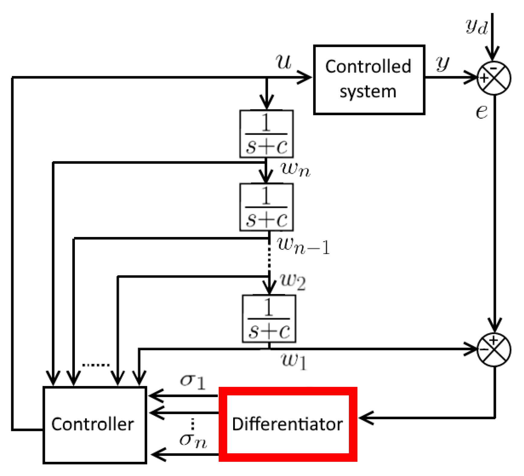
The biggest advantage of the differentiator-based controllers proposed in [9,10,22] is that the controller requires no universal approximators, such as neural net or fuzzy system, irrespective of the intrinsic unstructured uncertainties in a controlled system. Studies typically adopted such approximators to capture unstructured uncertainties for controlling uncertain nonlinear systems (e.g., refer to [8,23,24,25,26,27,28,29] and the references therein). Thecontroller (24) is directly influenced by the performance of the differentiator. The block diagram of the overall closed-loop control system is illustrated in Figure 8.

Figure 8. Block diagram of the closed-loop control system.

In the following simulations, the controller constants are the same as $c=1$ and $g=25$, from which the vector $\mathbf{g}$ in (24) is calculated as $\mathbf{g}={[625,50]}^T$. All initial values of the controlled system, controller, and differentiators were set to zero. The same differentiators, that is, HOSD (8), (9), HOSMD (19), and HGO (20), were used in the following simulations. The parameters in the respective differentiators were selected so that the settling time of the system output was about 0.5 seconds under the condition that they all used the same controller constants (c and g).

3.2.1. First Simulation

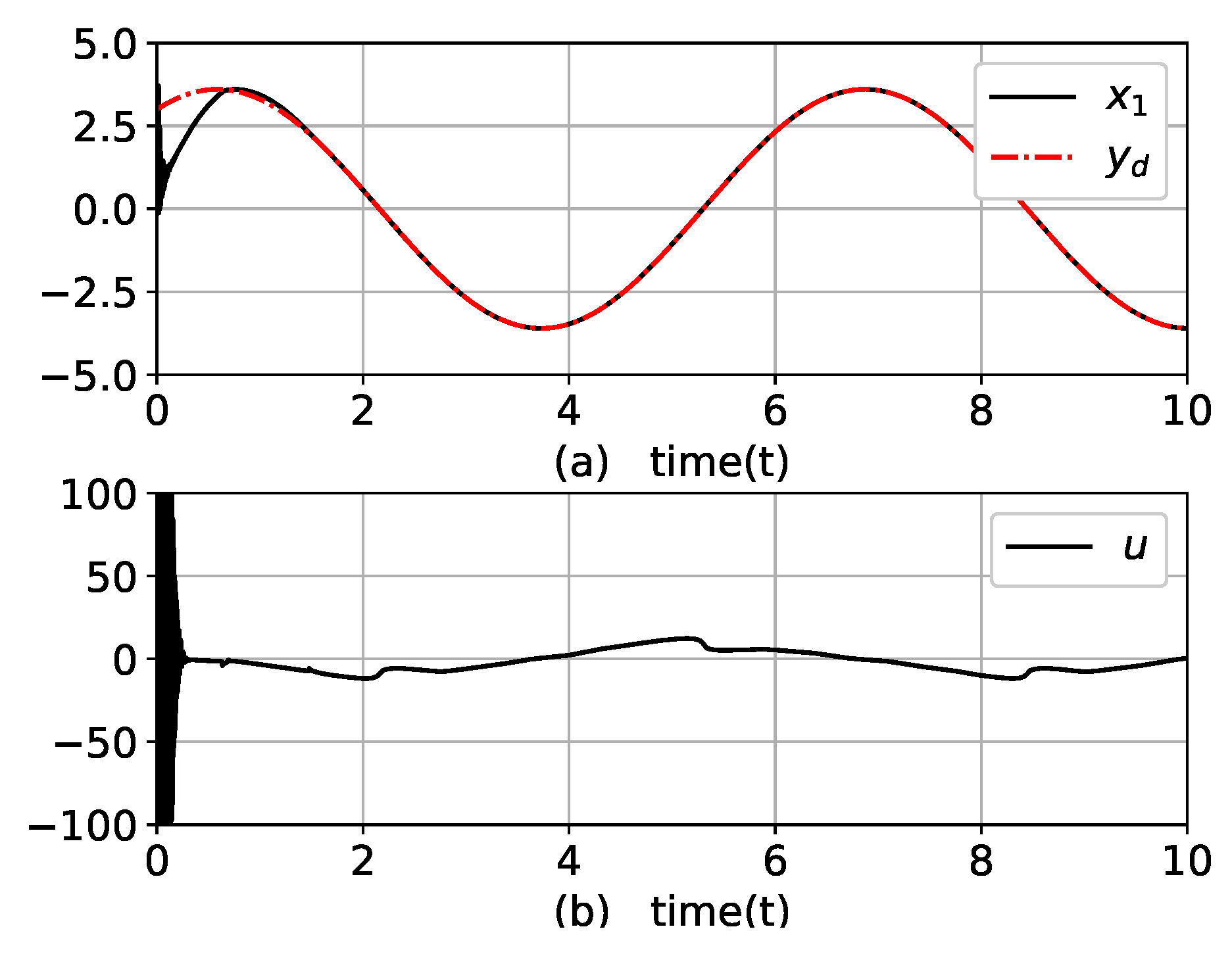
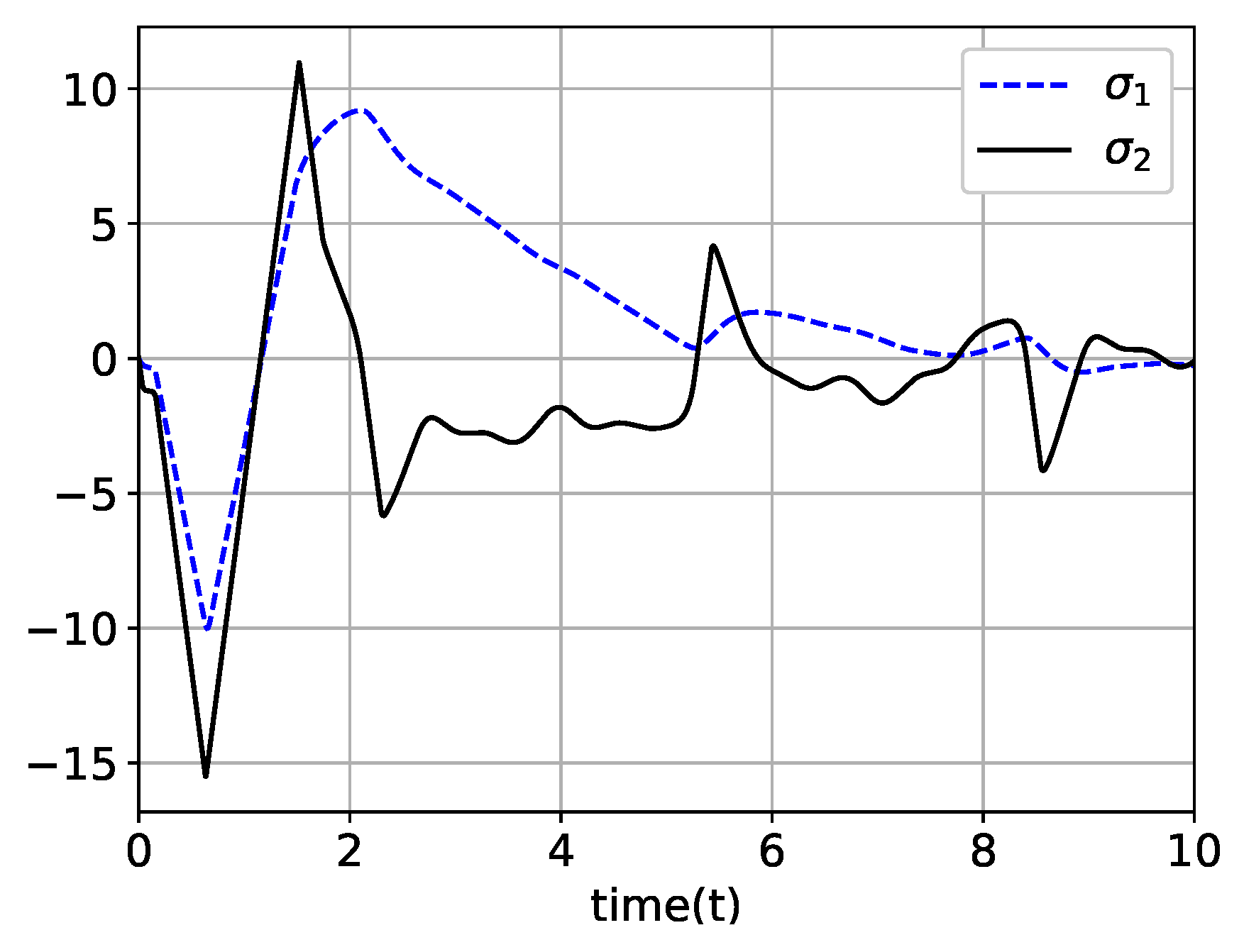
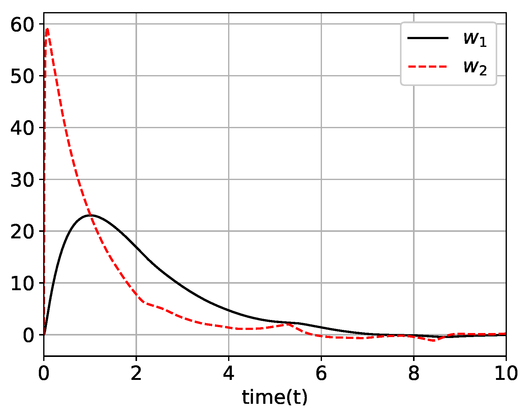
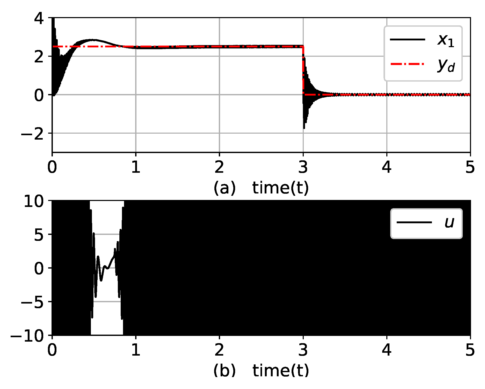
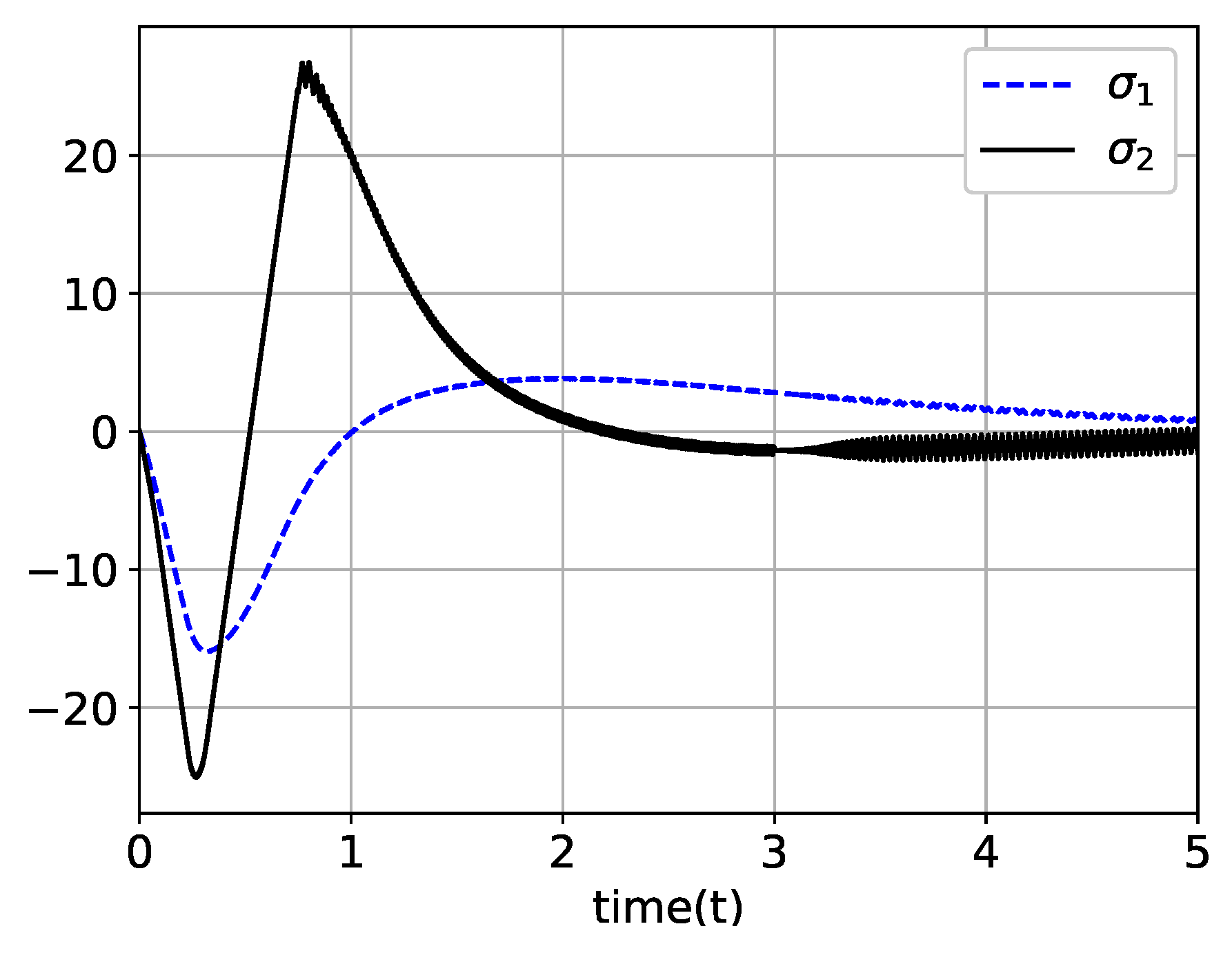
Tracking performance was compared using the desired output $y_d\left(t\right)=2sint+3cost$ in this subsection. Differentiator parameters are presented as ⓐ in Table 2. The simulation results with HOSD are shown in Figure 9, Figure 10 and Figure 11.

Table 2. Simulation parameter sets.

	HOSD	HOSDM	HGO
	controller constants: $c=1$, $g=50$
ⓐ	$k_1=k_2=30$	$M=500$	$c_0=3$, $c_1=3$
	$L_1=L_2=10,000$		$c_2=1$, $ϵ=0.1$
ⓑ	$k_1=k_2=30$	$M=30$	$c_0=3$, $c_1=3$
	$L_1=L_2=10,000$		$c_2=1$, $ϵ=0.1$

Figure 9. In the case of the proposed HOSD: (a) y, $y_d$ and (b) u.

Figure 10. The proposed HOSD: trajectories of ${\sigma }_1$ and ${\sigma }_2$.

Figure 11. The proposed HOSD: trajectories of $w_1$ and $w_2$.

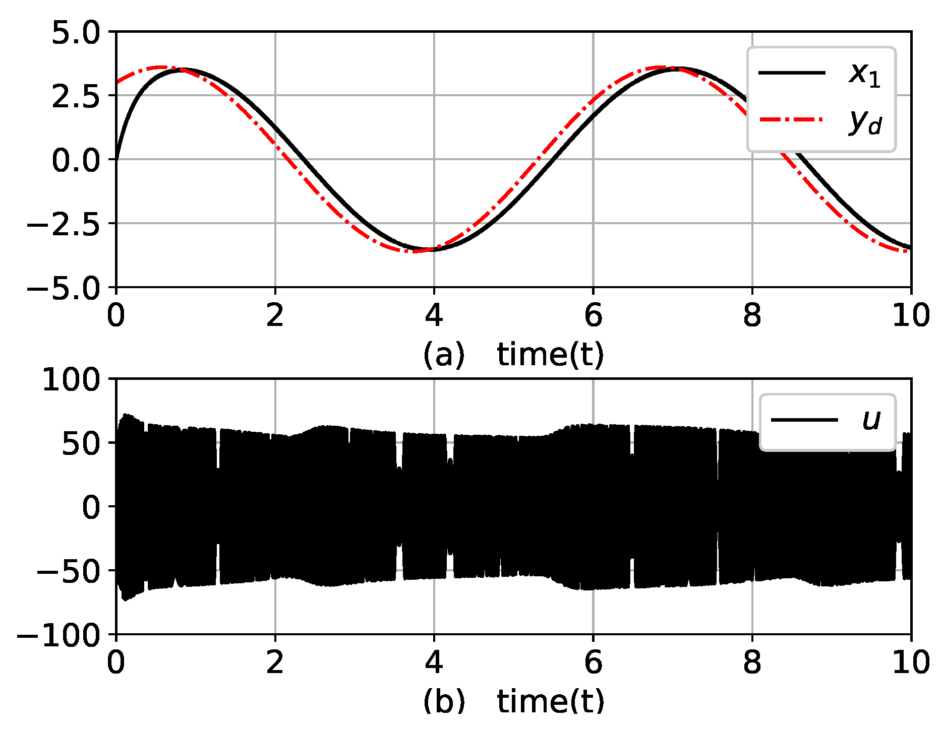
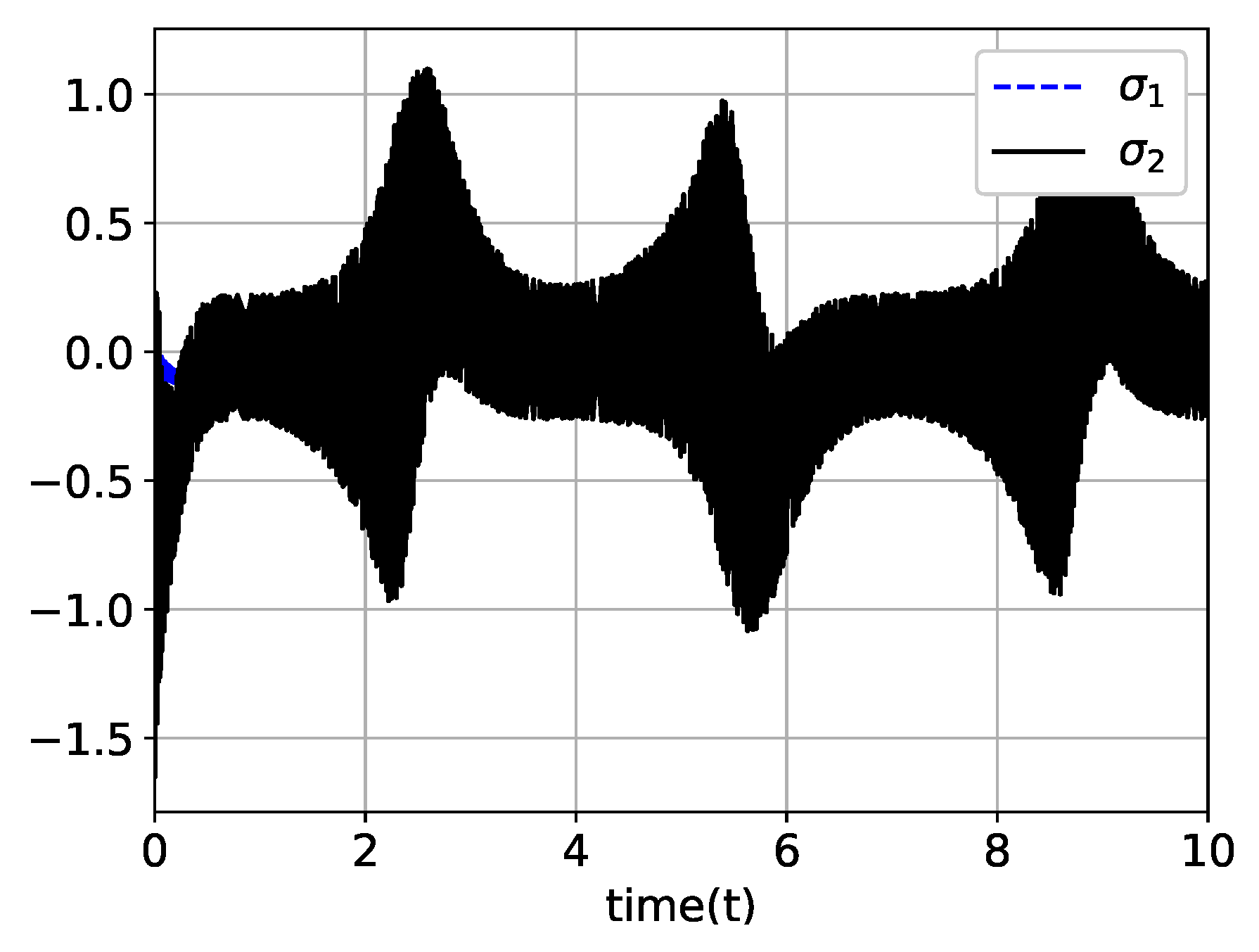
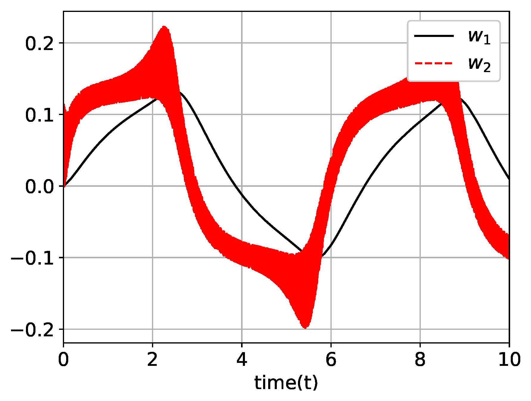
The simulation results ofr HOSMD are shown in Figure 12, Figure 13 and Figure 14. To meet the settling time restriction, a large M value was required and the input chattering was inevitable.

Figure 12. For HOSMD: (a) y, $y_d$, and (b) u.

Figure 13. For HOSMD: trajectories of ${\sigma }_1$ and ${\sigma }_2$.

Figure 14. For HOSMD: trajectories of $w_1$ and $w_2$.

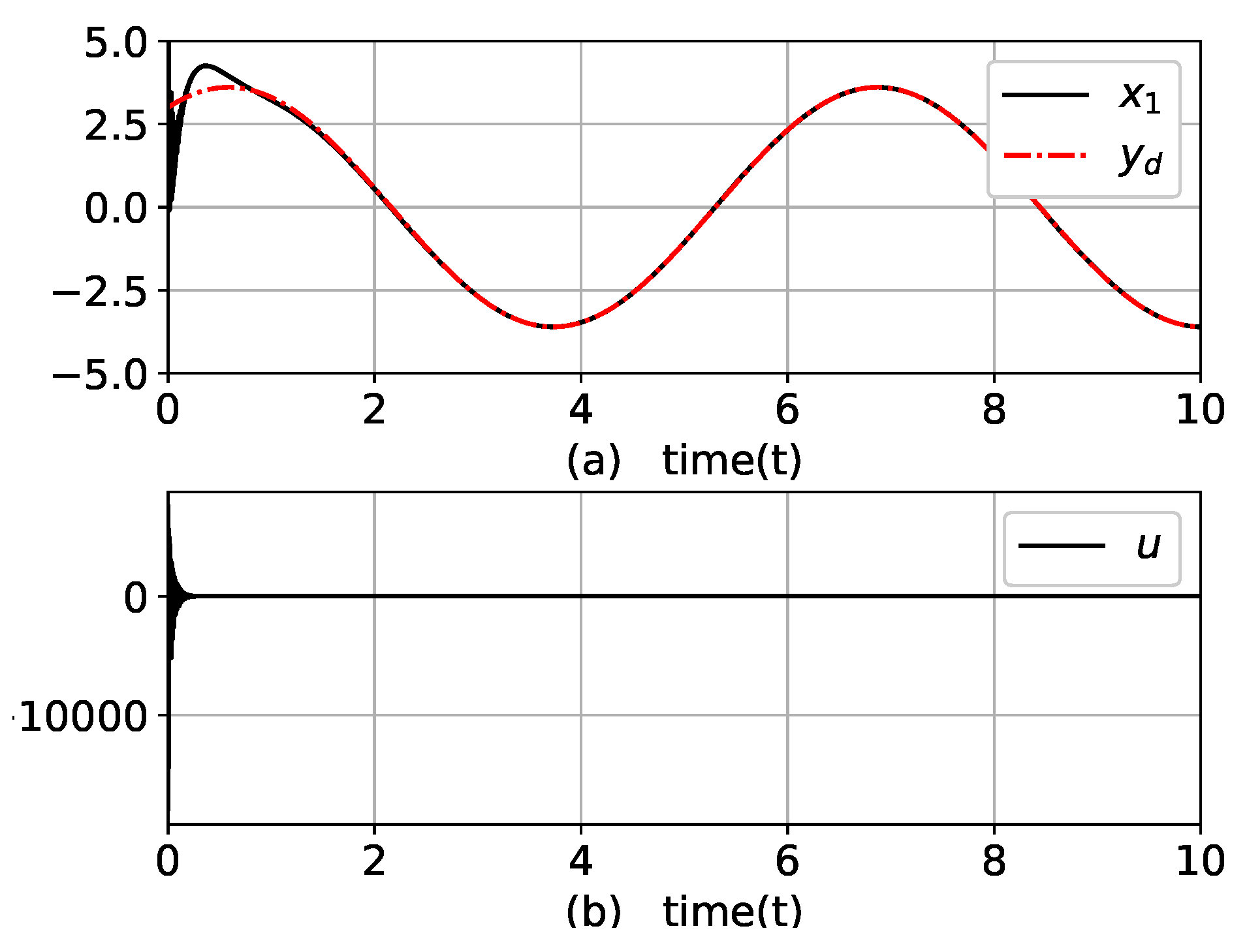
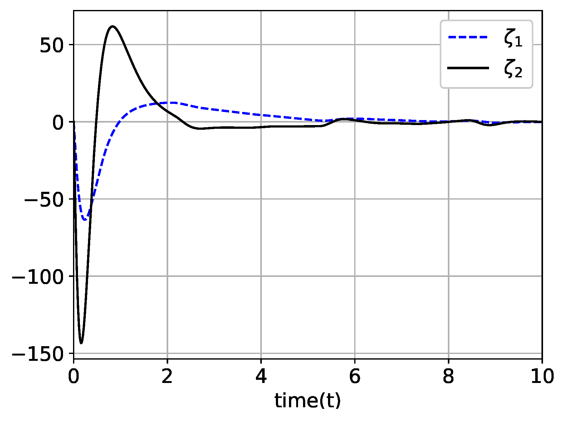
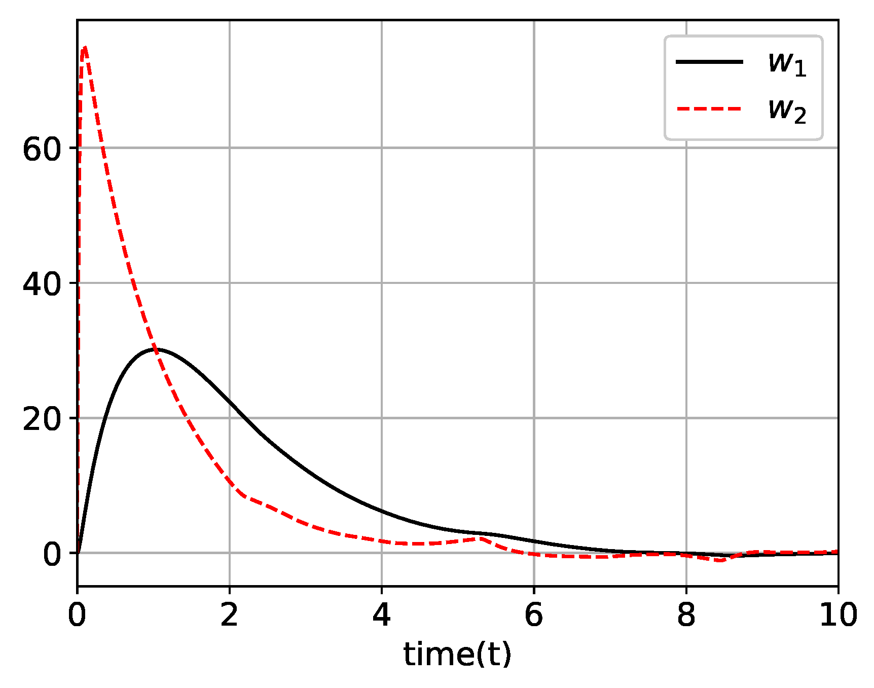
The simulation results with HGO are shown in Figure 15, Figure 16 and Figure 17. To meet the settling time restriction, a small $ϵ$ value was required and a huge peaking in the control input appeared.

Figure 15. For HGO: (a) y, $y_d$, and (b) u.

Figure 16. For HGO: trajectories of ${\sigma }_1$ and ${\sigma }_2$.

Figure 17. For HGO: trajectories of $w_1$ and $w_2$.

3.2.2. Second Simulation

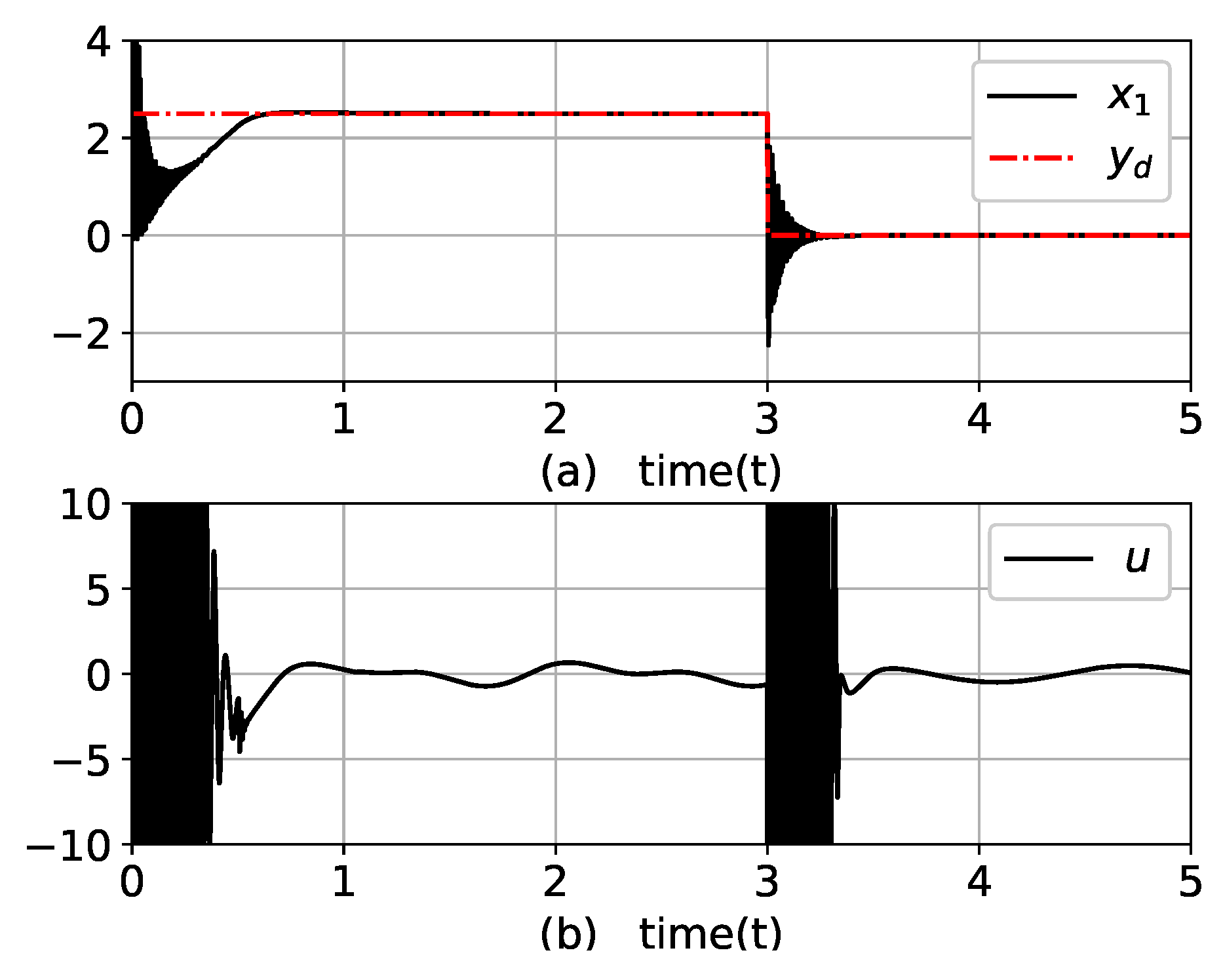
In this subsection, $y_d$ was moved abruptly at $t=0$ (since $x_1\left(0\right)=0$) and $t=3$ to check and compare the performance of the controllers. The difference of this simulation from the first simulation was that $y_d$ was harder to track because it changed abruptly at some time points. The selected parameters are presented in Table 2 ⓑ.

The simulation results with HOSMD are depicted in Figure 18 and Figure 19. For the specified settling time (0.5 s), the intensive chattering in the control input was inevitable in the case of HOSMD.

Figure 18. For HOSMD: (a) y, $y_d$, and (b) u.

Figure 19. For HOSMD: trajectories of ${\sigma }_1$ and ${\sigma }_2$.

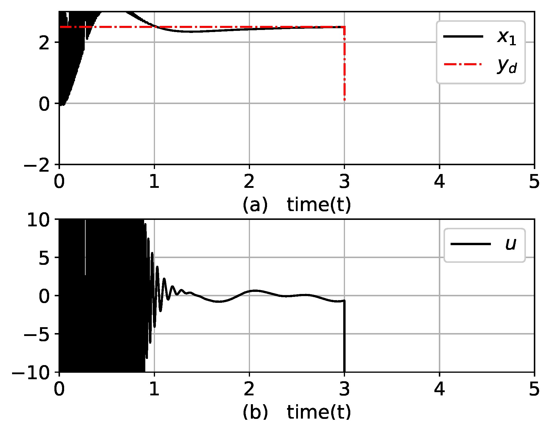
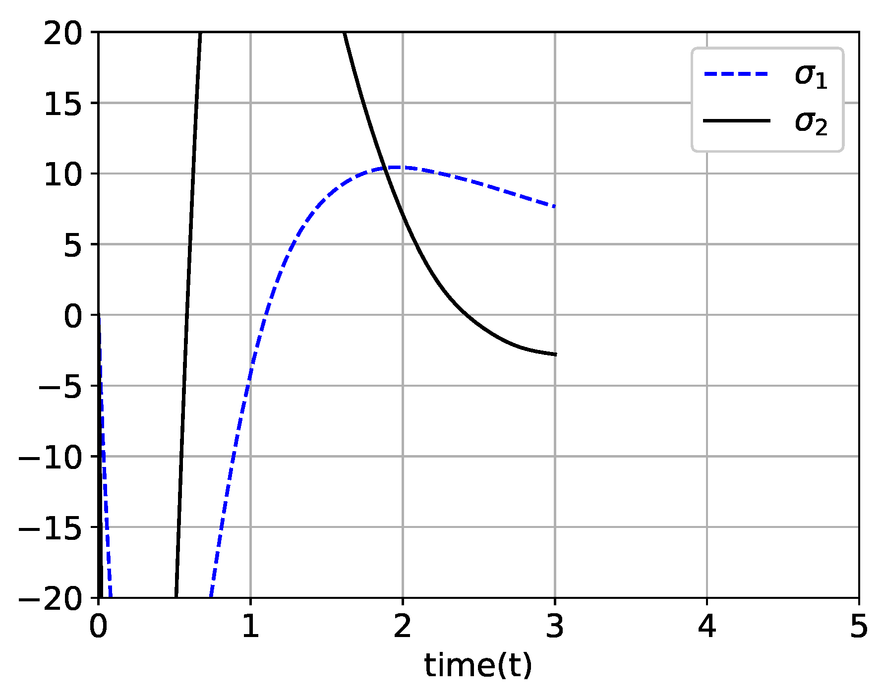
For HGO, the simulation results are depicted in Figure 20 and Figure 21. In this case, the parameters needed to meet the settling time of 0.5 s were not found. For a better controller performance, the value of $ϵ$ must be smaller, resulting in instability as well as control chattering. As shown in Figure 20, even with a relatively large $ϵ(=0.1)$ value, the system output diverged at $t=3$.

Figure 20. In the case of HGO: (a) y, $y_d$, and (b) u.

Figure 21. For HGO, trajectories of ${\sigma }_1$ and ${\sigma }_2$.

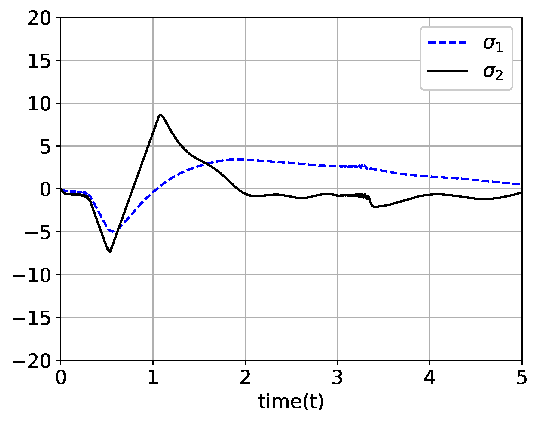
The simulation results for the proposed HOSD are depicted in Figure 22 and Figure 23. In this case, the specified settling time (0.5 s) was clearly met and the output of the system tracked the desired one well. Besides the inevitable short periods of chattering after the abrupt changes in $y_d$, no severe chattering was observedd in the control input and ${\sigma }_2$.

Figure 22. For the proposed HOSD: (a) y, $y_d$, and (b) u.

Figure 23. For the proposed HOSD: trajectories of ${\sigma }_1$ and ${\sigma }_2$.

4. Conclusions

A novel HOSD that can asymptotically track higher-order time-derivatives of a signal was proposed. Based on a prior study [19], the result was extended to the case of higher-order derivative estimations. We proved by successively applying the generalized Barbalat’s lemma that the estimations of higher-order time-derivatives of a signal approach zero asymptotically. Its dynamic equations are relatively simple. No chattering or peaking was shown in the estimations. In the simulations, the proposed HOSD performed better than existing widely used differentiators, such as HOSMD or HGO, when was used in the estimations of higher-order time-derivatives of a signal.

References

- Han, J. From PID to Active Disturbance Control. IEEE Trans. Ind. Electron. 2009, 56, 900–906. [Google Scholar] [CrossRef]
- Belanger, P.R.; Dobrovolny, P.; Helmy, A.; Zhang, X. Estimation of Angular Velocity and Acceleration from Shaft-Encoder Measurements. Int. J. Robot. Res. 1998, 17, 1225–1233. [Google Scholar] [CrossRef]
- Khalil, H.K. High-Gain Observers in Feedback Control: Application to Permanent Magnet Synchronous Motors. IEEE Control Syst. Mag. 2017, 37, 25–41. [Google Scholar]
- Levant, A. Non-homogeneous finite-time-convergent differentiator. In Proceedings of the 48th IEEE Conference on Decision and Control, Shanghai, China, 15–18 December 2009; pp. 8399–8404. [Google Scholar]
- Carneiro, J.F.; Almeida, F.G.D. On the Influence of Velocity and Acceleration Estimators on a Servopneumatic System Behaviour. IEEE Access 2016, 4, 6541–6553. [Google Scholar] [CrossRef]
- Gao, Z. Active Disturbance Rejection Control: A Paradigm Shift in Feedback Control Design. In Proceedings of the 2006 American Control Conference, Minneapolis, MN, USA, 14–16 June 2006. [Google Scholar]
- Efimov, D.; Zolghadri, A.; Raissi, T. Actuator fault detection and compensation under feedback control. Automatica 2011, 47, 1699–1705. [Google Scholar] [CrossRef]
- Park, J.-H.; Kim, S.-H.; Park, T.-S. Output-Feedback Adaptive Neural Controller for Uncertain Pure-Feedback Nonlinear Systems Using a High-Order Sliding Mode Observer. IEEE Trans. Neural Netw. Learn. Syst. 2019, 5, 1596–1601. [Google Scholar] [CrossRef] [PubMed]
- Park, J.-H.; Kim, S.-H.; Park, T.-S. Approximation-Free Output-Feedback Non-Backstepping Controller for Uncertain SISO Nonautonomous Nonlinear Pure-Feedback Systems. Mathematics 2019, 7, 456. [Google Scholar] [CrossRef]
- Park, J.-H.; Kim, S.-H.; Park, T.-S. Approximation-Free State-Feedback Backstepping Controller for Uncertain Pure-Feedback Nonautonomous Nonlinear Systems Based on Time-Derivative Estimator. IEEE Access 2019, 7, 126634–126641. [Google Scholar] [CrossRef]
- Levant, A. Robust Exact Differentiation via Sliding Mode Technique. Automatica 1998, 34, 379–384. [Google Scholar] [CrossRef]
- Levant, A. Universal Single-Input–Single-Output (SISO) Sliding-Mode Controllers with Finite-Time Convergence. IEEE Trans. Autom. Control 2001, 46, 1147–1451. [Google Scholar] [CrossRef]
- Levant, A. Higher-order sliding modes, differentiation and output-feedback control. Int. J. Control 2003, 76, 924–941. [Google Scholar] [CrossRef]
- Wang, X.; Chen, Z.; Yang, G. Finite-Time-Convergent Differentiator Based on Singular Perturbation Technique. IEEE Trans. Autom. Control 2007, 52, 1731–1737. [Google Scholar] [CrossRef]
- Ibrir, S. Linear time-derivative trackers. Automatica 2004, 40, 397–405. [Google Scholar] [CrossRef]
- Khalil, H.K. Cascade high-gain observers in output feedback control. Automatica 2017, 80, 110–118. [Google Scholar] [CrossRef]
- Angulo, M.T.; Moreno, J.A.; Fridman, L. Robust exact uniformly convergent arbitrary order differentiator. Automatica 2013, 49, 2489–2495. [Google Scholar] [CrossRef]
- Shao, X.; Liu, J.; Li, J.; Cao, H.; Shen, C.; Zhang, X. Augmented nonlinear differentiator design and application to nonlinear uncertain systems. ISA Trans. 2017, 67, 30–46. [Google Scholar] [CrossRef]
- Park, J.-H.; Kim, S.-H.; Park, T.-S. Asymptotically convergent switching differentiator. Int. J. Adapt. Control Signal Process. 2019, 33, 557–566. [Google Scholar] [CrossRef]
- Su, Y.; Huang, J. Stability of a Class of Linear Switching Systems with Application to Two Consensus Problems. IEEE Trans. Autom. Control 2012, 57, 1420–1430. [Google Scholar] [CrossRef]
- Hunter, J.D. Matplotlib: A 2D graphics environment. Comput. Sci. Eng. 2007, 9, 90–95. [Google Scholar] [CrossRef]
- Park, J.-H.; Kim, S.-H.; Park, T.-S. Approximation-Free Output-Feedback Control of Uncertain Nonlinear Systems Using Higher-Order Sliding Mode Observer. J. Dyn. Syst. Meas. Control 2018, 140, 124502-1–124502-5. [Google Scholar] [CrossRef]
- Park, J.-H.; Huh, S.-H.; Kim, S.-H.; Seo, S.-J.; Park, G.-T. Direct Adaptive Controller for Nonaffine Nonlinear Systems Using Self-Structuring Neural Networks. IEEE Trans. Neural Netw. 2005, 16, 414–422. [Google Scholar] [CrossRef]
- Park, J.-H.; Kim, S.-H.; Moon, C.-J. Adaptive Neural Control for Strict-Feedback Nonlinear Systems without Backstepping. IEEE Trans. Neural Netw. 2009, 20, 1204–1209. [Google Scholar] [CrossRef]
- Park, J.-H.; Park, G.-T.; Kim, S.-H.; Moon, C.-J. Direct Adaptive Self-Structuring Fuzzy Controller for Nonaffine Nonlinear Systems. Fuzzy Sets Syst. 2005, 153, 429–445. [Google Scholar] [CrossRef]
- Park, J.-H.; Park, G.-T.; Kim, S.-H.; Moon, C.-J. Output-feedback control of uncertain nonlinear systems using a self-structuring adaptive fuzzy observer. Fuzzy Sets Syst. 2005, 151, 21–42. [Google Scholar] [CrossRef]
- Park, J.-H.; Kim, S.-H. Direct Adaptive Output-Feedback Fuzzy Controller for Nonaffine Nonlinear System. IEE Proc. Control Theory Appl. 2004, 151, 65–72. [Google Scholar] [CrossRef]
- Park, J.-H.; Park, G.-T. Robust Adaptive Fuzzy Controller for Nonaffine Nonlinear Systems with Dynamic Rule Activation. Int. J. Robust Nonlinear Control 2003, 13, 117–139. [Google Scholar] [CrossRef]
- Park, J.-H.; Park, G.-T. Robust adaptive fuzzy controller for nonlinear system using estimation of bounds for approximation errors. Fuzzy Sets Syst. 2003, 133, 19–36. [Google Scholar] [CrossRef]
© 2020 by the authors. Licensee MDPI, Basel, Switzerland. This article is an open access article distributed under the terms and conditions of the Creative Commons Attribution (CC BY) license (http://creativecommons.org/licenses/by/4.0/).